
Hydroclimatic Impact Assessment Using the SWAT Model in India—State of the Art Review


Abstract
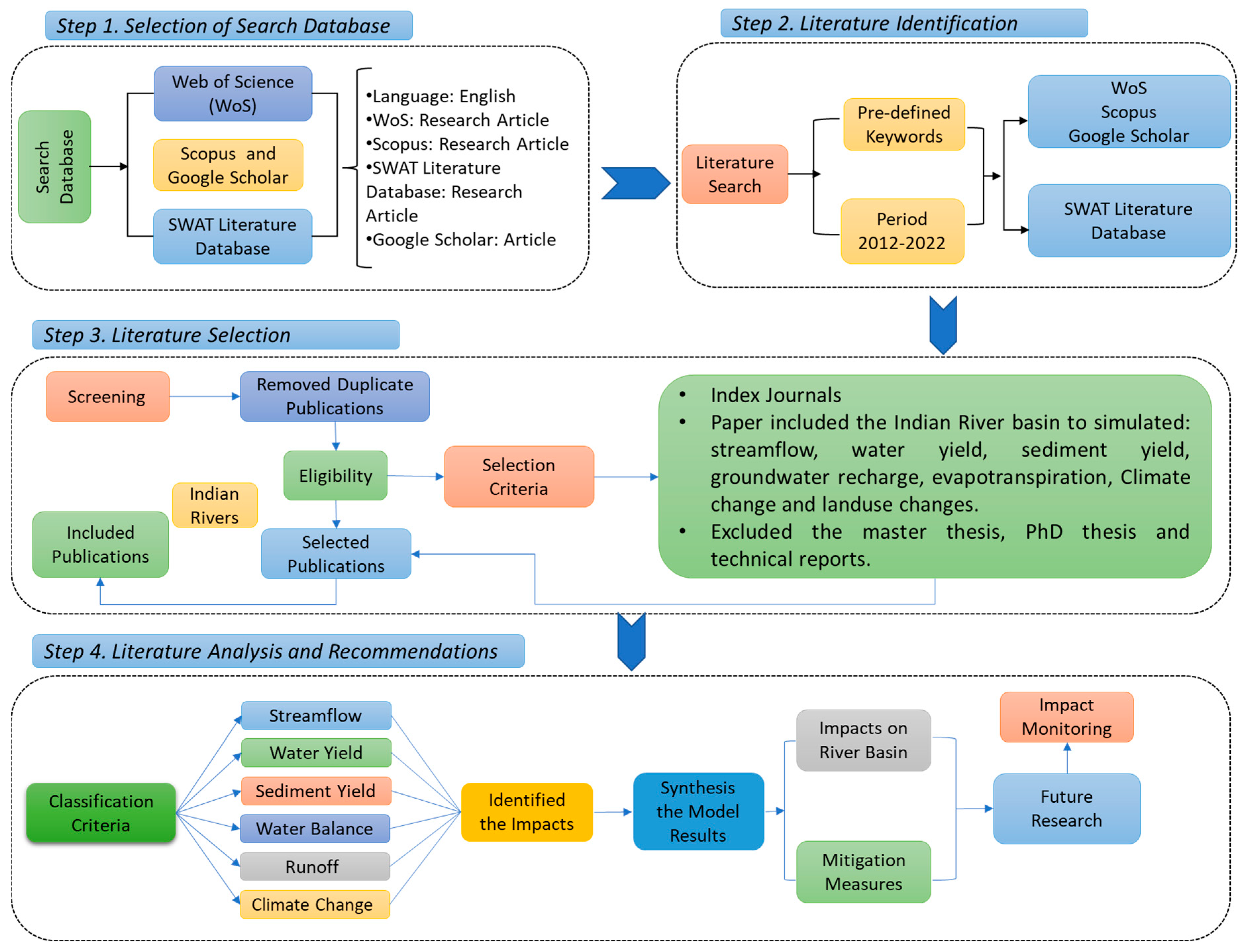
:1. Introduction
2. A General Framework of SWAT-Based Climate Change Studies
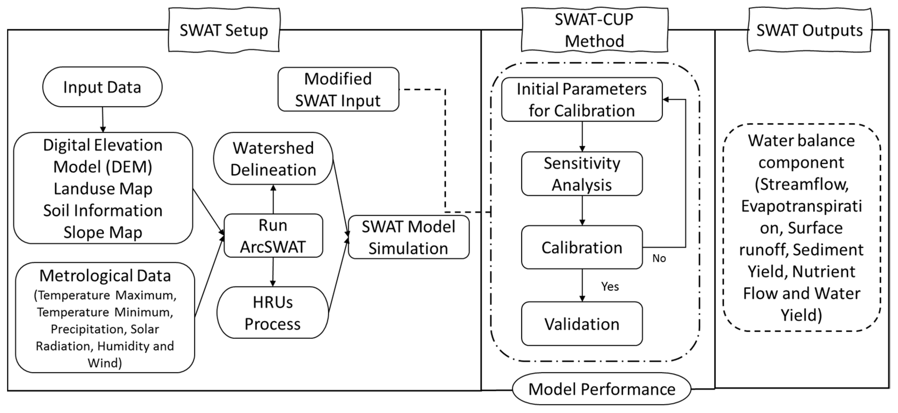
2.1. SWAT Setup, Calibration, and Validation
2.2. Climate Projections
2.3. Bias Correction of Climate Projections
3. SWAT-Based Climate Change Studies
3.1. SWAT-Based Climate Change Studies in Different Parts of the World
3.2. SWAT-Based Climate Change Studies in India
3.3. The SWAT’s Performance in India
3.3.1. Sensitivity Analysis
3.3.2. Streamflow Performance
4. Challenges and Future Directions
5. Conclusions
Supplementary Materials
Author Contributions
Funding
Institutional Review Board Statement
Informed Consent Statement
Data Availability Statement
Acknowledgments
Conflicts of Interest
References
- Trenberth, K.E.; Jones, P.D.; Ambenje, P.; Bojariu, R.; Easterling, D.; Klein Tank, A.; Parker, D.; Rahimzadeh, F.; Renwick, J.A.; Rusticucci, M.; et al. Observations: Surface and Atmospheric Climate Change. In Climate Change 2007: The Physical Science Basis; Solomon, S., Qin, D., Manning, M., Chen, Z., Marquis, M., Averyt, K.B., Tignor, M., Miller, H.L., Eds.; Cambridge University Press: Cambridge, UK; New York, NY, USA, 2007; pp. 236–336. [Google Scholar]
- Ye, X.; Zhang, Q.; Liu, J.; Li, X.; Xu, C. Distinguishing the relative impacts of climate change and human activities on variation of streamflow in the Poyang Lake catchment, China. J. Hydrol. 2013, 494, 83–95. [Google Scholar] [CrossRef]
- Ouyang, Y.; Leininger, T.D.; Moran, M. Estimating Effects of Reforestation on Nitrogen and Phosphorus Load Reductions in the Lower Yazoo River Watershed, Mississippi. Ecol. Eng. 2015, 75, 449–456. [Google Scholar] [CrossRef]
- Shrestha, S.; Sharma, S.; Gupta, R.; Bhattarai, R. Impact of Global Climate Change on Stream Low Flows: A Case Study of the Great Miami River Watershed, Ohio, USA. Int. J. Agric. Biol. Eng. 2019, 12, 84–95. [Google Scholar] [CrossRef]
- Gampe, D.; Nikulin, G.; Ludwig, R. Using an ensemble of regional climate models to assess climate change impacts on water scarcity in European river basins. Sci. Total Environ. 2016, 573, 1503–1518. [Google Scholar] [CrossRef] [PubMed]
- Leta, O.T.; El-Kadi, A.I.; Dulai, H.; Ghazal, K.A. Assessment of climate change impacts on water balance components of Heeia watershed in Hawaii. J. Hydrol. Reg. Stud. 2016, 8, 182–197. [Google Scholar] [CrossRef]
- Okwala, T.; Shrestha, S.; Ghimire, S.; Mohanasundaram, S.; Datta, A. Assessment of climate change impacts on water balance and hydrological extremes in Bang Pakong-Prachin Buri river basin, Thailand. Environ. Res. 2020, 186, 109544. [Google Scholar] [CrossRef]
- Ayers, J.; Ficklin, D.L.; Stewart, I.T.; Strunk, M. Comparison of CMIP3 and CMIP5 Projected Hydrologic Conditions over the Upper Colorado River Basin. Int. J. Climatol. 2016, 36, 3807–3818. [Google Scholar] [CrossRef]
- Chattopadhyay, S.; Jha, M.K. Hydrological Response Due to Projected Climate Variability in Haw River Watershed, North Carolina, USA. Hydrol. Sci. 2016, 61, 495–506. [Google Scholar] [CrossRef]
- Yan, T.; Bai, J.; Arsenio, T.; Liu, J.; Shen, Z. Future Climate Change Impacts on Streamflow and Nitrogen Exports Based on CMIP5 Projection in the Miyun Reservoir Basin, China. Ecohydrol. Hydrobiol. 2019, 19, 266–278. [Google Scholar] [CrossRef]
- Zhang, A.; Liu, W.; Yin, Z.; Fu, G.; Zheng, C. How Will Climate Change Affect the Water Availability in the Heihe River Basin, Northwest China? J. Hydrometeorol. 2016, 17, 1517–1542. [Google Scholar] [CrossRef]
- Verma, A.K.; Jha, M.K. Evaluation of a GIS-Based Watershed Model for Streamflow and Sediment-Yield Simulation in the Upper Baitarani River Basin of Eastern India. J. Hydrol. Eng. 2015, 20, C5015001. [Google Scholar] [CrossRef]
- Tan, M.L.; Gassman, P.W.; Yang, X.; Haywood, J. A Review of SWAT Applications, Performance and Future Needs for Simulation of Hydro-Climatic Extremes. Adv. Water Resour. 2020, 143, 103662. [Google Scholar] [CrossRef]
- Chen, C.; Gan, R.; Feng, D.; Yang, F.; Zuo, Q. Quantifying the Contribution of SWAT Modeling and CMIP6 Inputting to Streamflow Prediction Uncertainty under Climate Change. J. Clean. Prod. 2022, 364, 132675. [Google Scholar] [CrossRef]
- Khoi, D.N.; Thang, L.V. Climate Change Impacts on Streamflow and Non-Point Source Pollutant Loads in the 3S Rivers of the Mekong Basin. Water Environ. J. 2017, 31, 401–409. [Google Scholar] [CrossRef]
- Mishra, Y.; Nakamura, T.; Babel, M.S.; Ninsawat, S.; Ochi, S. Impact of Climate Change on Water Resources of the Bheri River Basin, Nepal. Water 2018, 10, 220. [Google Scholar] [CrossRef]
- Masud, M.B.; Ferdous, J.; Faramarzi, M. Projected Changes in Hydrological Variables in the Agricultural Region of Alberta, Canada. Water 2018, 10, 1810. [Google Scholar] [CrossRef]
- Teshager, A.D.; Gassman, P.W.; Secchi, S.; Schoof, J.T.; Misgna, G. Modeling Agricultural Watersheds with the Soil and Water Assessment Tool (SWAT): Calibration and Validation with a Novel Procedure for Spatially Explicit HRUs. Environ. Manag. 2016, 57, 894–911. [Google Scholar] [CrossRef]
- Abbaspour, K.C.; Rouholahnejad, E.; Vaghefi, S.; Srinivasan, R.; Yang, H.; Kløve, B. A Continental-Scale Hydrology and Water Quality Model for Europe: Calibration and Uncertainty of a High-Resolution Large-Scale SWAT Model. J. Hydrol. 2015, 524, 733–752. [Google Scholar] [CrossRef]
- Arnold, J.G.; Moriasi, D.N.; Gassman, P.W.; Abbaspour, K.C.; White, M.J.; Srinivasan, R.; Santhi, C.; Harmel, R.D.; Van Griensven, A.; Van Liew, M.W. SWAT: Model Use, Calibration, and Validation. Trans. ASABE 2012, 55, 1491–1508. [Google Scholar] [CrossRef]
- Gassman, P.W.; Reyes, M.R.; Green, C.H.; Arnold, J.G. The Soil and Water Assessment Tool: Historical Development, Applications, and Future Research Directions. Trans. ASABE 2007, 50, 1211–1250. [Google Scholar] [CrossRef]
- Wang, X.; Li, Z.; Li, M. Impacts of Climate Change on Stream Flow and Water Quality in a Drinking Water Source Area, Northern China. Environ. Earth Sci. 2018, 77, 410. [Google Scholar] [CrossRef]
- Arnold, J.G.; Srinivasan, R.; Muttiah, R.S.; Williams, J.R. Large Area Hydrologic Modeling and Assessment Part I: Model Development 1. JAWRA J. Am. Water Resour. Assoc. 1998, 34, 73–89. [Google Scholar] [CrossRef]
- Tan, M.L.; Gassman, P.W.; Srinivasan, R.; Arnold, J.G.; Yang, X. A review of SWAT studies in Southeast Asia: Applications, challenges and future directions. Water 2019, 11, 914. [Google Scholar] [CrossRef]
- Jha, M.K.; Gassman, P.W.; Panagopoulos, Y. Regional Changes in Nitrate Loadings in the Upper Mississippi River Basin under Predicted Mid-Century Climate. Reg. Environ. Chang. 2015, 15, 449–460. [Google Scholar] [CrossRef]
- Sood, A.; Muthuwatta, L.; McCartney, M. A SWAT Evaluation of the Effect of Climate Change on the Hydrology of the Volta River Basin. Water Int. 2013, 38, 297–311. [Google Scholar] [CrossRef]
- Tan, M.L.; Yusop, Z.; Chua, V.P.; Chan, N.W. Climate Change Impacts under CMIP5 RCP Scenarios on Water Resources of the Kelantan River Basin, Malaysia. Atmos. Res. 2017, 189, 1–10. [Google Scholar] [CrossRef]
- Githui, F.; Gitau, W.; Mutua, F.; Bauwens, W. Climate Change Impact on SWAT Simulated Streamflow in Western Kenya. Int. J. Climatol. 2009, 29, 1823–1834. [Google Scholar] [CrossRef]
- Shrestha, B.; Babel, M.S.; Maskey, S.; van Griensven, A.; Uhlenbrook, S.; Green, A.; Akkharath, I. Impact of Climate Change on Sediment Yield in the Mekong River Basin: A Case Study of the Nam Ou Basin, Lao PDR. Hydrol. Earth Syst. Sci. 2013, 17, 1–20. [Google Scholar] [CrossRef]
- Neupane, R.P.; Yao, J.; White, J.D. Estimating the Effects of Climate Change on the Intensification of Monsoonal-Driven Stream Discharge in a Himalayan Watershed. Hydrol. Process. 2014, 28, 6236–6250. [Google Scholar] [CrossRef]
- Nath, A.; Samanta, S.; Banerjee, S.; Danda, A.A.; Hazra, S. Threat of arsenic contamination, salinity and water pollution in agricultural practices of Sundarban Delta, India, and mitigation strategies. SN Appl. Sci. 2021, 3, 560. [Google Scholar] [CrossRef]
- Misra, A.K. Impact of Urbanization on the Hydrology of Ganga Basin (India). Water Resour. Manag. 2011, 25, 705–719. [Google Scholar] [CrossRef]
- Borah, L.; Kalita, B.; Boro, P.; Kulnu, A.S.; Hazarika, N. Climate Change Impacts on Socio-Hydrological Spaces of the Brahmaputra Floodplain in Assam, Northeast India: A Review. Front. Water 2022, 4, 913840. [Google Scholar] [CrossRef]
- Srinivasan, R.; Ramanarayanan, T.S.; Arnold, J.G.; Bednarz, S.T. Large Area Hydrologic Modeling and Assessment Part II: Model Application 1. JAWRA J. Am. Water Resour. Assoc. 1998, 34, 91–101. [Google Scholar] [CrossRef]
- Zhang, X.; Srinivasan, R.; Van Liew, M. Multi-Site Calibration of the SWAT Model for Hydrologic Modeling. Trans. ASABE 2008, 51, 2039–2049. [Google Scholar] [CrossRef]
- Arnold, J.G.; Muttiah, R.S.; Srinivasan, R.; Allen, P.M. Regional Estimation of Base Flow and Groundwater Recharge in the Upper Mississippi River Basin. J. Hydrol. 2000, 227, 21–40. [Google Scholar] [CrossRef]
- Arnold, J.G.; Allen, P.M.; Bernhardt, G. A Comprehensive Surface-Groundwater Flow Model. J. Hydrol. 1993, 142, 47–69. [Google Scholar] [CrossRef]
- Anand, J.; Gosain, A.K.; Khosa, R. Prediction of Land Use Changes Based on Land Change Modeler and Attribution of Changes in the Water Balance of Ganga Basin to Land Use Change Using the SWAT Model. Sci. Total Environ. 2018, 644, 503–519. [Google Scholar] [CrossRef]
- Chanapathi, T.; Thatikonda, S.; Raghavan, S. Analysis of Rainfall Extremes and Water Yield of Krishna River Basin under Future Climate Scenarios. J. Hydrol. Reg. Stud. 2018, 19, 287–306. [Google Scholar] [CrossRef]
- Chinnasamy, P.; Muthuwatta, L.; Eriyagama, N.; Pavelic, P.; Lagudu, S. Modeling the Potential for Floodwater Recharge to Offset Groundwater Depletion: A Case Study from the Ramganga Basin, India. Sustain. Water Resour. Manag. 2018, 4, 331–344. [Google Scholar] [CrossRef]
- Nilawar, A.P.; Waikar, M.L. Use of SWAT to Determine the Effects of Climate and Land Use Changes on Streamflow and Sediment Concentration in the Purna River Basin, India. Environ. Earth Sci. 2018, 77, 783. [Google Scholar] [CrossRef]
- Rahman, K.; Ray, N.; Giuliani, G.; Maringanti, C.; George, C.; Lehmann, A. Breaking Walls towards Fully Open Source Hydrological Modeling. Water Resour. 2017, 44, 23–30. [Google Scholar] [CrossRef]
- Shen, Z.Y.; Chen, L.; Chen, T. Analysis of Parameter Uncertainty in Hydrological and Sediment Modeling Using GLUE Method: A Case Study of SWAT Model Applied to Three Gorges Reservoir Region, China. Hydrol. Earth Syst. Sci. 2012, 16, 121–132. [Google Scholar] [CrossRef]
- Visakh, S.; Raju, P.V.; Kulkarni, S.S.; Diwakar, P.G. Inter-Comparison of Water Balance Components of River Basins Draining into Selected Delta Districts of Eastern India. Sci. Total Environ. 2019, 654, 1258–1269. [Google Scholar] [CrossRef] [PubMed]
- Abbaspour, K.C.; Vaghefi, S.A.; Srinivasan, R. A Guideline for Successful Calibration and Uncertainty Analysis for Soil and Water Assessment: A Review of Papers from the 2016 International SWAT Conference. Water 2018, 10, 6. [Google Scholar] [CrossRef]
- Park, G.A.; Park, J.Y.; Joh, H.K.; Lee, J.W.; Ahn, S.R.; Kim, S.J. Evaluation of Mixed Forest Evapotranspiration and Soil Moisture Using Measured and Swat Simulated Results in a Hillslope Watershed. KSCE J. Civ. Eng. 2014, 18, 315–322. [Google Scholar] [CrossRef]
- Amatya, D.M.; Jha, M.K. Evaluating the SWAT Model for a Low-Gradient Forested Watershed in Coastal South Carolina. Trans. ASABE 2011, 54, 2151–2163. [Google Scholar] [CrossRef]
- Abbas, N.; Wasimi, S.A.; Al-Ansari, N.; Nasrin Baby, S. Recent Trends and Long-Range Forecasts of Water Resources of Northeast Iraq and Climate Change Adaptation Measures. Water 2018, 10, 1562. [Google Scholar] [CrossRef]
- Moriasi, D.N.; Arnold, J.G.; Van Liew, M.W.; Bingner, R.L.; Harmel, R.D.; Veith, T.L. Model Evaluation Guidelines for Systematic Quantification of Accuracy in Watershed Simulations. Trans. ASABE 2007, 50, 885–900. [Google Scholar] [CrossRef]
- Krause, P.; Boyle, D.P.; Bäse, F. Comparison of Different Efficiency Criteria for Hydrological Model Assessment. Adv. Geosci. 2005, 5, 89–97. [Google Scholar] [CrossRef]
- Moriasi, D.N.; Gitau, M.W.; Pai, N.; Daggupati, P. Hydrologic and Water Quality Models: Performance Measures and Evaluation Criteria. Trans. ASABE 2015, 58, 1763–1785. [Google Scholar]
- Nash, J.E.; Sutcliffe, J.V. River Flow Forecasting through Conceptual Models Part I—A Discussion of Principles. J. Hydrol. 1970, 10, 282–290. [Google Scholar] [CrossRef]
- Gupta, H.V.; Sorooshian, S.; Yapo, P.O. Status of Automatic Calibration for Hydrologic Models: Comparison with Multilevel Expert Calibration. J. Hydrol. Eng. 1999, 4, 135–143. [Google Scholar] [CrossRef]
- Parry, M.; Parry, M.L.; Canziani, O.; Palutikof, J.; Van der Linden, P.; Hanson, C. Climate Change 2007-Impacts, Adaptation and Vulnerability: Working Group II Contribution to the Fourth Assessment Report of the IPCC; Cambridge University Press: Cambridge, UK, 2007. [Google Scholar]
- Reddy, K.R.; Hodges, H.F. Climate Change and Global Crop Productivity; CABI: Wallingford, UK, 2000. [Google Scholar]
- Suppiah, R.; Hennessy, K.J.; Whetton, P.H.; McInnes, K.; Macadam, I.; Bathols, J.; Ricketts, J.; Page, C.M. Australian Climate Change Projections Derived from Simulations Performed for the IPCC 4th Assessment Report. Aust. Meteorol. Mag. 2007, 56, 131–152. [Google Scholar]
- Thomas, A. Agricultural Irrigation Demand under Present and Future Climate Scenarios in China. Glob. Planet. Chang. 2008, 60, 306–326. [Google Scholar] [CrossRef]
- Bonan, G.B.; Oleson, K.W.; Vertenstein, M.; Levis, S.; Zeng, X.; Dai, Y.; Dickinson, R.E.; Yang, Z.-L. The Land Surface Climatology of the Community Land Model Coupled to the NCAR Community Climate Model. J. Clim. 2002, 15, 3123–3149. [Google Scholar] [CrossRef]
- Salinger, M.J.; Stigter, C.J.; Das, H.P. Agrometeorological Adaptation Strategies to Increasing Climate Variability and Climate Change. Agric. For. Meteorol. 2000, 103, 167–184. [Google Scholar] [CrossRef]
- Cuculeanu, V.; Tuinea, P.; Bălteanu, D. Climate Change Impacts in Romania: Vulnerability and Adaptation Options. GeoJournal 2002, 57, 203–209. [Google Scholar] [CrossRef]
- Ghimire, U.; Srinivasan, G.; Agarwal, A. Assessment of Rainfall Bias Correction Techniques for Improved Hydrological Simulation. Int. J. Climatol. 2019, 39, 2386–2399. [Google Scholar] [CrossRef]
- Turner, S.W.; Galelli, S. Water Supply Sensitivity to Climate Change: An R Package for Implementing Reservoir Storage Analysis in Global and Regional Impact Studies. Environ. Model. Softw. 2016, 76, 13–19. [Google Scholar] [CrossRef]
- Hay, L.E.; Wilby, R.L.; Leavesley, G.H. A Comparison of Delta Change and Downscaled GCM Scenarios for Three Mountainous Basins in the United States 1. JAWRA J. Am. Water Resour. Assoc. 2000, 36, 387–397. [Google Scholar] [CrossRef]
- Hay, L.E.; Clark, M.P. Use of Statistically and Dynamically Downscaled Atmospheric Model Output for Hydrologic Simulations in Three Mountainous Basins in the Western United States. J. Hydrol. 2003, 282, 56–75. [Google Scholar] [CrossRef]
- Schmidli, J.; Frei, C.; Vidale, P.L. Downscaling from GCM Precipitation: A Benchmark for Dynamical and Statistical Downscaling Methods. Int. J. Climatol. 2006, 26, 679–689. [Google Scholar] [CrossRef]
- Fowler, H.J.; Kilsby, C.G. Using Regional Climate Model Data to Simulate Historical and Future River Flows in Northwest England. Clim. Chang. 2007, 80, 337–367. [Google Scholar] [CrossRef]
- Sharma, D.; Das Gupta, A.; Babel, M.S. Spatial Disaggregation of Bias-Corrected GCM Precipitation for Improved Hydrologic Simulation: Ping River Basin, Thailand. Hydrol. Earth Syst. Sci. 2007, 11, 1373–1390. [Google Scholar] [CrossRef]
- Moron, V.; Robertson, A.W.; Ward, M.N.; Ndiaye, O. Weather Types and Rainfall over Senegal. Part II: Downscaling of GCM Simulations. J. Clim. 2008, 21, 288–307. [Google Scholar] [CrossRef]
- Piani, C.; Weedon, G.P.; Best, M.; Gomes, S.M.; Viterbo, P.; Hagemann, S.; Haerter, J.O. Statistical Bias Correction of Global Simulated Daily Precipitation and Temperature for the Application of Hydrological Models. J. Hydrol. 2010, 395, 199–215. [Google Scholar] [CrossRef]
- Sun, F.; Roderick, M.L.; Lim, W.H.; Farquhar, G.D. Hydroclimatic Projections for the Murray-Darling Basin Based on an Ensemble Derived from Intergovernmental Panel on Climate Change AR4 Climate Models. Water Resour. Res. 2011, 47, W00G02. [Google Scholar] [CrossRef]
- Wood, A.W.; Leung, L.R.; Sridhar, V.; Lettenmaier, D.P. Hydrologic Implications of Dynamical and Statistical Approaches to Downscaling Climate Model Outputs. Clim. Chang. 2004, 62, 189–216. [Google Scholar] [CrossRef]
- Gudmundsson, L.; Bremnes, J.B.; Haugen, J.E.; Engen-Skaugen, T. Downscaling RCM Precipitation to the Station Scale Using Statistical Transformations–a Comparison of Methods. Hydrol. Earth Syst. Sci. 2012, 16, 3383–3390. [Google Scholar] [CrossRef]
- Hanel, M.; Mrkvičková, M.; Máca, P.; Vizina, A.; Pech, P. Evaluation of Simple Statistical Downscaling Methods for Monthly Regional Climate Model Simulations with Respect to the Estimated Changes in Runoff in the Czech Republic. Water Resour. Manag. 2013, 27, 5261–5279. [Google Scholar] [CrossRef]
- Tiwari, P.R.; Kar, S.C.; Mohanty, U.C.; Dey, S.; Sinha, P.; Raju, P.V.S.; Shekhar, M.S. On the Dynamical Downscaling and Bias Correction of Seasonal-Scale Winter Precipitation Predictions over North India. Q. J. R. Meteorol. Soc. 2016, 142, 2398–2410. [Google Scholar] [CrossRef]
- Buser, C.M.; Künsch, H.R.; Lüthi, D.; Wild, M.; Schär, C. Bayesian Multi-Model Projection of Climate: Bias Assumptions and Interannual Variability. Clim. Dyn. 2009, 33, 849–868. [Google Scholar] [CrossRef]
- Haddeland, I.; Heinke, J.; Voß, F.; Eisner, S.; Chen, C.; Hagemann, S.; Ludwig, F. Effects of Climate Model Radiation, Humidity and Wind Estimates on Hydrological Simulations. Hydrol. Earth Syst. Sci. 2012, 16, 305–318. [Google Scholar] [CrossRef]
- Jakob Themeßl, M.; Gobiet, A.; Leuprecht, A. Empirical-Statistical Downscaling and Error Correction of Daily Precipitation from Regional Climate Models. Int. J. Climatol. 2011, 31, 1530–1544. [Google Scholar] [CrossRef]
- Haerter, J.O.; Eggert, B.; Moseley, C.; Piani, C.; Berg, P. Statistical Precipitation Bias Correction of Gridded Model Data Using Point Measurements. Geophys. Res. Lett. 2015, 42, 1919–1929. [Google Scholar] [CrossRef]
- Kumar Mishra, B.; Herath, S. Assessment of Future Floods in the Bagmati River Basin of Nepal Using Bias-Corrected Daily GCM Precipitation Data. J. Hydrol. Eng. 2015, 20, 05014027. [Google Scholar] [CrossRef]
- Nyunt, C.T.; Koike, T.; Yamamoto, A. Statistical Bias Correction for Climate Change Impact on the Basin Scale Precipitation in Sri Lanka, Philippines, Japan and Tunisia. Hydrol. Earth Syst. Sci. Discuss. 2016, preprint. [Google Scholar] [CrossRef]
- Kumar, N.; Tischbein, B.; Kusche, J.; Laux, P.; Beg, M.K.; Bogardi, J.J. Impact of Climate Change on Water Resources of Upper Kharun Catchment in Chhattisgarh, India. J. Hydrol. Reg. Stud. 2017, 13, 189–207. [Google Scholar] [CrossRef]
- Saharia, A.M.; Sarma, A.K. Future Climate Change Impact Evaluation on Hydrologic Processes in the Bharalu and Basistha Basins Using SWAT Model. Nat. Hazards 2018, 92, 1463–1488. [Google Scholar] [CrossRef]
- Pandey, B.K.; Khare, D.; Kawasaki, A.; Mishra, P.K. Climate Change Impact Assessment on Blue and Green Water by Coupling of Representative CMIP5 Climate Models with Physical Based Hydrological Model. Water Resour. Manag. 2019, 33, 141–158. [Google Scholar] [CrossRef]
- Nilawar, A.P.; Waikar, M.L. Impacts of Climate Change on Streamflow and Sediment Concentration under RCP 4.5 and 8.5: A Case Study in Purna River Basin, India. Sci. Total Environ. 2019, 650, 2685–2696. [Google Scholar] [CrossRef]
- Chanapathi, T.; Thatikonda, S.; Keesara, V.R.; Ponguru, N.S. Assessment of water resources and crop yield under future climate scenarios: A case study in a Warangal district of Telangana, India. J. Earth Syst. Sci. 2020, 129, 20. [Google Scholar] [CrossRef]
- Alcamo, J.; Dronin, N.; Endejan, M.; Golubev, G.; Kirilenko, A. A New Assessment of Climate Change Impacts on Food Production Shortfalls and Water Availability in Russia. Glob. Environ. Chang. 2007, 17, 429–444. [Google Scholar] [CrossRef]
- Hanjra, M.A.; Qureshi, M.E. Global Water Crisis and Future Food Security in an Era of Climate Change. Food Policy 2010, 35, 365–377. [Google Scholar] [CrossRef]
- Cohen, S.J.; Miller, K.A.; Hamlet, A.F.; Avis, W. Climate Change and Resource Management in the Columbia River Basin. Water Int. 2000, 25, 253–272. [Google Scholar] [CrossRef]
- Tung, C. Climate Change Impacts on Water Resources of the Tsengwen Creek Watershed in Taiwan 1. JAWRA J. Am. Water Resour. Assoc. 2001, 37, 167–176. [Google Scholar] [CrossRef]
- Payne, J.T.; Wood, A.W.; Hamlet, A.F.; Palmer, R.N.; Lettenmaier, D.P. Mitigating the Effects of Climate Change on the Water Resources of the Columbia River Basin. Clim. Chang. 2004, 62, 233–256. [Google Scholar] [CrossRef]
- Zhang, G.-H.; Nearing, M.A.; Liu, B.-Y. Potential Effects of Climate Change on Rainfall Erosivity in the Yellow River Basin of China. Trans. ASAE 2005, 48, 511–517. [Google Scholar] [CrossRef]
- Wilby, R.L.; Harris, I. A Framework for Assessing Uncertainties in Climate Change Impacts: Low-Flow Scenarios for the River Thames, UK. Water Resour. Res. 2006, 42, W02419. [Google Scholar] [CrossRef]
- Wurbs, R.A.; Muttiah, R.S.; Felden, F. Incorporation of Climate Change in Water Availability Modeling. J. Hydrol. Eng. 2005, 10, 375–385. [Google Scholar] [CrossRef]
- Moss, R.H.; Edmonds, J.A.; Hibbard, K.A.; Manning, M.R.; Rose, S.K.; Van Vuuren, D.P.; Carter, T.R.; Emori, S.; Kainuma, M.; Kram, T. The next Generation of Scenarios for Climate Change Research and Assessment. Nature 2010, 463, 747–756. [Google Scholar] [CrossRef]
- White, C.J.; McInnes, K.L.; Cechet, R.P.; Corney, S.P.; Grose, M.R.; Holz, G.K.; Katzfey, J.J.; Bindoff, N.L. On Regional Dynamical Downscaling for the Assessment and Projection of Temperature and Precipitation Extremes across Tasmania, Australia. Clim. Dyn. 2013, 41, 3145–3165. [Google Scholar] [CrossRef]
- Pinto, I.; Lennard, C.; Tadross, M.; Hewitson, B.; Dosio, A.; Nikulin, G.; Panitz, H.-J.; Shongwe, M.E. Evaluation and Projections of Extreme Precipitation over Southern Africa from Two CORDEX Models. Clim. Chang. 2016, 135, 655–668. [Google Scholar] [CrossRef]
- Akhtar, M.; Ahmad, N.; Booij, M.J. The Impact of Climate Change on the Water Resources of Hindukush–Karakorum–Himalaya Region under Different Glacier Coverage Scenarios. J. Hydrol. 2008, 355, 148–163. [Google Scholar] [CrossRef]
- Diallo, I.; Sylla, M.B.; Giorgi, F.; Gaye, A.T.; Camara, M. Multimodel GCM-RCM Ensemble-Based Projections of Temperature and Precipitation over West Africa for the Early 21st Century. Int. J. Geophys. 2012, 2012, 972896. [Google Scholar] [CrossRef]
- Mote, P.W.; Salathé, E.P. Future Climate in the Pacific Northwest. Clim. Chang. 2010, 102, 29–50. [Google Scholar] [CrossRef]
- Sharma, D.; Babel, M.S. Application of Downscaled Precipitation for Hydrological Climate-Change Impact Assessment in the Upper Ping River Basin of Thailand. Clim. Dyn. 2013, 41, 2589–2602. [Google Scholar] [CrossRef]
- Huisman, J.A.; Breuer, L.; Bormann, H.; Bronstert, A.; Croke, B.F.W.; Frede, H.-G.; Gräff, T.; Hubrechts, L.; Jakeman, A.J.; Kite, G. Assessing the Impact of Land Use Change on Hydrology by Ensemble Modeling (LUCHEM) III: Scenario Analysis. Adv. Water Resour. 2009, 32, 159–170. [Google Scholar] [CrossRef]
- Zhang, A.; Zhang, C.; Fu, G.; Wang, B.; Bao, Z.; Zheng, H. Assessments of Impacts of Climate Change and Human Activities on Runoff with SWAT for the Huifa River Basin, Northeast China. Water Resour. Manag. 2012, 26, 2199–2217. [Google Scholar] [CrossRef]
- Marhaento, H.; Booij, M.J.; Hoekstra, A.Y. Hydrological Response to Future Land-Use Change and Climate Change in a Tropical Catchment. Hydrol. Sci. 2018, 63, 1368–1385. [Google Scholar] [CrossRef]
- Emami, F.; Koch, M. Modeling the Impact of Climate Change on Water Availability in the Zarrine River Basin and Inflow to the Boukan Dam, Iran. Climate 2019, 7, 51. [Google Scholar] [CrossRef]
- Nazari-Sharabian, M.; Taheriyoun, M.; Ahmad, S.; Karakouzian, M.; Ahmadi, A. Water Quality Modeling of Mahabad Dam Watershed–Reservoir System under Climate Change Conditions, Using SWAT and System Dynamics. Water 2019, 11, 394. [Google Scholar] [CrossRef]
- Sowjanya, P.N.; Reddy, V.K.; Shashi, M. Intra- and Interannual Streamflow Variations of Wardha Watershed under Changing Climate. ISH J. Hydraul. Eng. 2020, 26, 197–208. [Google Scholar] [CrossRef]
- Sarthi, P.P.; Kumar, P.; Ghosh, S. Possible Future Rainfall over Gangetic Plains (GP), India, in Multi-Model Simulations of CMIP3 and CMIP5. Theor. Appl. Climatol. 2016, 124, 691–701. [Google Scholar] [CrossRef]
- Bhatla, R.; Ghosh, S.; Mall, R.K.; Sinha, P.; Sarkar, A. Regional Climate Model Performance in Simulating Intra-Seasonal and Interannual Variability of Indian Summer Monsoon. Pure Appl. Geophys. 2018, 175, 3697–3718. [Google Scholar] [CrossRef]
- Mishra, A.K.; Dwivedi, S.; Das, S. Role of Arabian Sea Warming on the Indian Summer Monsoon Rainfall in a Regional Climate Model. Int. J. Climatol. 2020, 40, 2226–2238. [Google Scholar] [CrossRef]
- Kundu, S.; Khare, D.; Mondal, A. Individual and Combined Impacts of Future Climate and Land Use Changes on the Water Balance. Ecol. Eng. 2017, 105, 42–57. [Google Scholar] [CrossRef]
- Singh, V.; Goyal, M.K. Curve Number Modifications and Parameterization Sensitivity Analysis for Reducing Model Uncertainty in Simulated and Projected Streamflows in a Himalayan Catchment. Ecol. Eng. 2017, 108, 17–29. [Google Scholar] [CrossRef]
- Islam, A.K.M.; Paul, S.; Mohammed, K.; Billah, M.; Fahad, M.; Rabbani, G.; Hasan, M.; Islam, G.M.; Bala, S.K. Hydrological Response to Climate Change of the Brahmaputra Basin Using CMIP5 General Circulation Model Ensemble. J. Water Clim. Chang. 2018, 9, 434–448. [Google Scholar] [CrossRef]
- Bhuvaneswari, K.; Geethalakshmi, V.; Lakshmanan, A.; Srinivasan, R.; Sekhar, N.U. The Impact of El Niño/Southern Oscillation on Hydrology and Rice Productivity in the Cauvery Basin, India: Application of the Soil and Water Assessment Tool. Weather Clim. Extrem. 2013, 2, 39–47. [Google Scholar] [CrossRef]
- Narsimlu, B.; Gosain, A.K.; Chahar, B.R. Assessment of Future Climate Change Impacts on Water Resources of Upper Sind River Basin, India Using SWAT Model. Water Resour. Manag. 2013, 27, 3647–3662. [Google Scholar] [CrossRef]
- Chandra, P.; Patel, P.L.; Porey, P.D.; Gupta, I.D. Estimation of Sediment Yield Using SWAT Model for Upper Tapi Basin. ISH J. Hydraul. Eng. 2014, 20, 291–300. [Google Scholar] [CrossRef]
- Pandey, A.; Lalrempuia, D.; Jain, S.K. Assessment of Hydropower Potential Using Spatial Technology and SWAT Modelling in the Mat River, Southern Mizoram, India. Hydrol. Sci. 2015, 60, 1651–1665. [Google Scholar] [CrossRef]
- Pervez, M.S.; Henebry, G.M. Assessing the Impacts of Climate and Land Use and Land Cover Change on the Freshwater Availability in the Brahmaputra River Basin. J. Hydrol. Reg. Stud. 2015, 3, 285–311. [Google Scholar] [CrossRef]
- Kumar, N.; Singh, S.K.; Srivastava, P.K.; Narsimlu, B. SWAT Model Calibration and Uncertainty Analysis for Streamflow Prediction of the Tons River Basin, India, using Sequential Uncertainty Fitting (SUFI-2) Algorithm.Model. Earth Syst. Environ. 2017, 3, 30. [Google Scholar] [CrossRef]
- Murty, P.S.; Pandey, A.; Suryavanshi, S. Application of Semi-Distributed Hydrological Model for Basin Level Water Balance of the Ken Basin of Central India. Hydrol. Process. 2014, 28, 4119–4129. [Google Scholar] [CrossRef]
- Abeysingha, N.S.; Singh, M.; Sehgal, V.K.; Khanna, M.; Pathak, H.; Jayakody, P.; Srinivasan, R. Assessment of Water Yield and Evapotranspiration over 1985 to 2010 in the Gomti River Basin in India Using the SWAT Model. Curr. Sci. 2015, 108, 2202–2212. [Google Scholar]
- Singh, A.; Imtiyaz, M.; Isaac, R.K.; Denis, D.M. Assessing the Performance and Uncertainty Analysis of the SWAT and RBNN Models for Simulation of Sediment Yield in the Nagwa Watershed, India. Hydrol. Sci. 2014, 59, 351–364. [Google Scholar] [CrossRef]
- Singh, A.; Imtiyaz, M.; Isaac, R.K.; Denis, D.M. Comparison of Soil and Water Assessment Tool (SWAT) and Multilayer Perceptron (MLP) Artificial Neural Network for Predicting Sediment Yield in the Nagwa Agricultural Watershed in Jharkhand, India. Agric. Water Manag. 2012, 104, 113–120. [Google Scholar] [CrossRef]
- Santra, P.; Das, B.S. Modeling Runoff from an Agricultural Watershed of Western Catchment of Chilika Lake through ArcSWAT. J. Hydro-Environ. Res. 2013, 7, 261–269. [Google Scholar] [CrossRef]
- Dutta, D.; Das, R.; Mazumdar, A. Assessment of Runoff and Sediment Yield in the Tilaya Reservoir, India Using SWAT Model. Asian J. Water Environ. Pollut. 2017, 14, 9–18. [Google Scholar] [CrossRef]
- Dutta, S.; Sen, D. Application of SWAT Model for Predicting Soil Erosion and Sediment Yield. Sustain. Water Resour. Manag. 2018, 4, 447–468. [Google Scholar] [CrossRef]
- Pandey, A.; Palmate, S.S. Assessing Future Water–Sediment Interaction and Critical Area Prioritization at Sub-Watershed Level for Sustainable Management. Paddy Water Environ. 2019, 17, 373–382. [Google Scholar] [CrossRef]
- Singh, L.; Saravanan, S. Evaluation of Blue and Green Water Using Combine Stream Flow and Soil Moisture Simulation in Wunna Watershed, India. Water Conser. Sci. Eng. 2022, 7, 211–225. [Google Scholar] [CrossRef]
- Singh, L.; Saravanan, S. Adaptation of Satellite-Based Precipitation Product to Study Runoff and Sediment of Indian River Watersheds. Arab. J. Geosci. 2022, 15, 326. [Google Scholar] [CrossRef]
- Singh, L.; Saravanan, S. Assessing Streamflow Modeling Using Single and Multi-Site Calibration Approach on Bharathpuzha Catchment, India: A Case Study. Model. Earth Syst. Environ. 2022, 8, 4135–4148. [Google Scholar] [CrossRef]
- Santra Mitra, S.; Kumar, A.; Santra, A.; Mitra, D.; Routh, S. Hydrological Modeling of Catchment Specific Runoff-Response to Variable Land-Use/Climatic Conditions and Trend-Based Hypothetical Scenario Generation: A Study on a Large River Basin in Eastern India. J. Indian Soc. Remote Sens. 2021, 49, 1895–1914. [Google Scholar] [CrossRef]
- Swain, S.S.; Mishra, A.; Chatterjee, C.; Sahoo, B. Climate-Changed versus Land-Use Altered Streamflow: A Relative Contribution Assessment Using Three Complementary Approaches at a Decadal Time-Spell. J. Hydrol. 2021, 596, 126064. [Google Scholar] [CrossRef]
- Nune, R.; George, B.A.; Western, A.W.; Garg, K.K.; Dixit, S.; Ragab, R. A Comprehensive Assessment Framework for Attributing Trends in Streamflow and Groundwater Storage to Climatic and Anthropogenic Changes: A Case Study in the Typical Semi-Arid Catchments of Southern India. Hydrol. Process. 2021, 35, e14305. [Google Scholar] [CrossRef]
- Horan, R.; Gowri, R.; Wable, P.S.; Baron, H.; Keller, V.D.; Garg, K.K.; Mujumdar, P.P.; Houghton-Carr, H.; Rees, G. A Comparative Assessment of Hydrological Models in the Upper Cauvery Catchment. Water 2021, 13, 151. [Google Scholar] [CrossRef]
- Desai, S.; Singh, D.K.; Islam, A.; Sarangi, A. Impact of Climate Change on the Hydrology of a Semi-Arid River Basin of India under Hypothetical and Projected Climate Change Scenarios. J. Water Clim. Chang. 2021, 12, 969–996. [Google Scholar] [CrossRef]
- Joseph, N.; Preetha, P.P.; Narasimhan, B. Assessment of Environmental Flow Requirements Using a Coupled Surface Water-Groundwater Model and a Flow Health Tool: A Case Study of Son River in the Ganga Basin. Ecol. Indic. 2021, 121, 107110. [Google Scholar] [CrossRef]
- Swain, S.S.; Mishra, A.; Sahoo, B.; Chatterjee, C. Water Scarcity-Risk Assessment in Data-Scarce River Basins under Decadal Climate Change Using a Hydrological Modelling Approach. J. Hydrol. 2020, 590, 125260. [Google Scholar] [CrossRef]
- Patil, N.S.; Nataraja, M. Effect of Land Use Land Cover Changes on Runoff Using Hydrological Model: A Case Study in Hiranyakeshi Watershed. Model. Earth Syst. Environ. 2020, 6, 2345–2357. [Google Scholar] [CrossRef]
- Shukla, A.K.; Ojha, C.S.P.; Garg, R.D.; Shukla, S.; Pal, L. Influence of Spatial Urbanization on Hydrological Components of the Upper Ganga River Basin, India. J. Hazard. Toxic Radioact. Waste 2020, 24, 04020028. [Google Scholar] [CrossRef]
- Setti, S.; Maheswaran, R.; Radha, D.; Sridhar, V.; Barik, K.K.; Narasimham, M.L. Attribution of Hydrologic Changes in a Tropical River Basin to Rainfall Variability and Land-Use Change: Case Study from India. J. Hydrol. Eng. 2020, 25, 05020015. [Google Scholar] [CrossRef]
- Venkatesh, K.; Krakauer, N.Y.; Sharifi, E.; Ramesh, H. Evaluating the Performance of Secondary Precipitation Products through Statistical and Hydrological Modeling in a Mountainous Tropical Basin of India. Adv. Meteorol. 2020, 2020, 8859185. [Google Scholar] [CrossRef]
- Padhiary, J.; Patra, K.C.; Dash, S.S.; Uday Kumar, A. Climate Change Impact Assessment on Hydrological Fluxes Based on Ensemble GCM Outputs: A Case Study in Eastern Indian River Basin. J. Water Clim. Chang. 2020, 11, 1676–1694. [Google Scholar] [CrossRef]
- Chauhan, N.; Kumar, V.; Paliwal, R. Quantifying the Impacts of Decadal Landuse Change on the Water Balance Components Using Soil and Water Assessment Tool in Ghaggar River Basin. SN Appl. Sci. 2020, 2, 1777. [Google Scholar] [CrossRef]
- Singh, L.; Saravanan, S. Simulation of Monthly Streamflow Using the SWAT Model of the Ib River Watershed, India. HydroResearch 2020, 3, 95–105. [Google Scholar] [CrossRef]
- Kanishka, G.; Eldho, T.I. Streamflow Estimation in Ungauged Basins Using Watershed Classification and Regionalization Techniques. J. Earth Syst. Sci. 2020, 129, 186. [Google Scholar] [CrossRef]
- Merina, R.N.; Sashikkumar, M.C.; Danesh, A.; Rizvana, N. Modelling Technique for Sediment Evaluation at Reservoir (South India). Water Resour. 2019, 46, 553–562. [Google Scholar] [CrossRef]
- Singh, V.; Sharma, A.; Goyal, M.K. Projection of Hydro-Climatological Changes over Eastern Himalayan Catchment by the Evaluation of RegCM4 RCM and CMIP5 GCM Models. Hydrol. Res. 2019, 50, 117–137. [Google Scholar] [CrossRef]
- Budamala, V.; Baburao Mahindrakar, A. Enhance the Prediction of Complex Hydrological Models by Pseudo-Simulators. Geocarto Int. 2021, 36, 1027–1043. [Google Scholar] [CrossRef]
- Bhattacharya, T.; Khare, D.; Arora, M. A Case Study for the Assessment of the Suitability of Gridded Reanalysis Weather Data for Hydrological Simulation in Beas River Basin of North Western Himalaya. Appl. Water Sci. 2019, 9, 110. [Google Scholar] [CrossRef]
- Paul, P.K.; Zhang, Y.; Mishra, A.; Panigrahy, N.; Singh, R. Comparative Study of Two State-of-the-Art Semi-Distributed Hydrological Models. Water 2019, 11, 871. [Google Scholar] [CrossRef]
- Adhikary, P.P.; Sena, D.R.; Dash, C.J.; Mandal, U.; Nanda, S.; Madhu, M.; Sahoo, D.C.; Mishra, P.K. Effect of Calibration and Validation Decisions on Streamflow Modeling for a Heterogeneous and Low Runoff–Producing River Basin in India. J. Hydrol. Eng. 2019, 24, 05019015. [Google Scholar] [CrossRef]
- Anshuman, A.; Kunnath-Poovakka, A.; Eldho, T.I. Towards the Use of Conceptual Models for Water Resource Assessment in Indian Tropical Watersheds under Monsoon-Driven Climatic Conditions. Environ. Earth Sci. 2019, 78, 282. [Google Scholar] [CrossRef]
- Adla, S.; Tripathi, S.; Disse, M. Can We Calibrate a Daily Time-Step Hydrological Model Using Monthly Time-Step Discharge Data? Water 2019, 11, 1750. [Google Scholar] [CrossRef]
- Ikhar, P.R.; Regulwar, D.G.; Kamodkar, R.U. Optimal Reservoir Operation Using Soil and Water Assessment Tool and Genetic Algorithm. ISH J. Hydraul. Eng. 2018, 24, 249–257. [Google Scholar] [CrossRef]
- Saini, M.; Dutta, V.; Singh, N.P.; Bajpai, O. Modeling and Assessing Land-Use and Hydrological Regimes to Future Land-Use Scenario for Sustainable Watershed Management in a Semi-Arid Region of Southern India. J. Environ. Sustain. 2018, 1, 393–409. [Google Scholar] [CrossRef]
- Tiwari, S.; Kar, S.C.; Bhatla, R.; Bansal, R. Temperature Index Based Snowmelt Runoff Modelling for the S Atluj R Iver Basin in the w Estern H Imalayas. Meteorol. Appl. 2018, 25, 302–313. [Google Scholar] [CrossRef]
- Sinha, R.K.; Eldho, T.I. Effects of Historical and Projected Land Use/Cover Change on Runoff and Sediment Yield in the Netravati River Basin, Western Ghats, India. Environ. Earth Sci. 2018, 77, 111. [Google Scholar] [CrossRef]
- Yaduvanshi, A.; Sharma, R.K.; Kar, S.C.; Sinha, A.K. Rainfall–Runoff Simulations of Extreme Monsoon Rainfall Events in a Tropical River Basin of India. Nat. Hazards 2018, 90, 843–861. [Google Scholar] [CrossRef]
- Goswami, S.B.; Bal, P.K.; Mitra, A.K. Use of Rainfall Forecast from a High-Resolution Global NWP Model in a Hydrological Stream Flow Model over Narmada River Basin during Monsoon. Model. Earth Syst. Environ. 2018, 4, 1029–1040. [Google Scholar] [CrossRef]
- Nagraj, S.P.; Nataraja, M.; Omprakash, T. Evaluation of Hydrological Components Using Hydrological Model SWAT for Malaprabha Subbasin. J. Geol. Soc. India 2018, 92, 195–200. [Google Scholar] [CrossRef]
- Shivhare, N.; Dikshit, P.K.S.; Dwivedi, S.B. A Comparison of Swat Model Calibration Techniques for Hydrological Modeling in the Ganga River Watershed. Engineering 2018, 4, 643–652. [Google Scholar] [CrossRef]
- Pati, A.; Sen, S.; Perumal, M. Modified Channel-Routing Scheme for SWAT Model. J. Hydrol. Eng. 2018, 23, 04018019. [Google Scholar] [CrossRef]
- Yaduvanshi, A.; Srivastava, P.; Worqlul, A.W.; Sinha, A.K. Uncertainty in a Lumped and a Semi-Distributed Model for Discharge Prediction in Ghatshila Catchment. Water 2018, 10, 381. [Google Scholar] [CrossRef]
- Himanshu, S.K.; Pandey, A.; Dayal, D. Evaluation of Satellite-Based Precipitation Estimates over an Agricultural Watershed of India. In Proceedings of the World Environmental and Water Resources Congress 2018: Watershed Management, Irrigation and Drainage, and Water Resources Planning and Management; American Society of Civil Engineers: Reston, VA, USA, 2018; pp. 308–320. [Google Scholar]
- Setti, S.; Rathinasamy, M.; Chandramouli, S. Assessment of Water Balance for a Forest Dominated Coastal River Basin in India Using a Semi Distributed Hydrological Model. Model. Earth Syst. Environ. 2018, 4, 127–140. [Google Scholar] [CrossRef]
- Hasan, M.A.; Pradhanang, S.M. Estimation of Flow Regime for a Spatially Varied Himalayan Watershed Using Improved Multi-Site Calibration of the Soil and Water Assessment Tool (SWAT) Model. Environ. Earth Sci. 2017, 76, 787. [Google Scholar] [CrossRef]
- Himanshu, S.K.; Pandey, A.; Shrestha, P. Application of SWAT in an Indian River Basin for Modeling Runoff, Sediment and Water Balance. Environ. Earth Sci. 2017, 76, 3. [Google Scholar] [CrossRef]
- Makwana, J.J.; Tiwari, M.K. Hydrological Stream Flow Modelling Using Soil and Water Assessment Tool (SWAT) and Neural Networks (NNs) for the Limkheda Watershed, Gujarat, India. Model. Earth Syst. Environ. 2017, 3, 635–645. [Google Scholar] [CrossRef]
- Suryavanshi, S.; Pandey, A.; Chaube, U.C. Hydrological Simulation of the Betwa River Basin (India) Using the SWAT Model. Hydrol. Sci. 2017, 62, 960–978. [Google Scholar] [CrossRef]
- Jothiprakash, V.; Praveenkumar, C.; Manasa, M. Daily Runoff Estimation in Musi River Basin, India, from Gridded Rainfall Using SWAT Model. Eur. Water 2017, 57, 63–69. [Google Scholar]
- Halefom, A.; Sisay, E.; Khare, D.; Singh, L.; Worku, T. Hydrological Modeling of Urban Catchment Using Semi-Distributed Model. Model. Earth Syst. Environ. 2017, 3, 683–692. [Google Scholar] [CrossRef]
- Kumar, N.; Tischbein, B.; Kusche, J.; Beg, M.K.; Bogardi, J.J. Impact of Land-Use Change on the Water Resources of the Upper Kharun Catchment, Chhattisgarh, India. Reg. Environ. Chang. 2017, 17, 2373–2385. [Google Scholar] [CrossRef]
- Abeysingha, N.S.; Singh, M.; Islam, A.; Sehgal, V.K. Climate Change Impacts on Irrigated Rice and Wheat Production in Gomti River Basin of India: A Case Study. SpringerPlus 2016, 5, 1250. [Google Scholar] [CrossRef]
- Alam, S.; Ali, M.M.; Islam, Z. Future Streamflow of Brahmaputra River Basin under Synthetic Climate Change Scenarios. J. Hydrol. Eng. 2016, 21, 05016027. [Google Scholar] [CrossRef]
- Patel, D.P.; Nandhakumar, N. Runoff Potential Estimation of Anjana Khadi Watershed Using SWAT Model in the Part of Lower Tapi Basin, West India. Sustain. Water Resour. Manag. 2016, 2, 103–118. [Google Scholar] [CrossRef]
- Babar, S.; Ramesh, H. Streamflow Response to Land Use–Land Cover Change over the Nethravathi River Basin, India. J. Hydrol. Eng. 2015, 20, 05015002. [Google Scholar] [CrossRef]
- Singh, D.; Jain, S.K.; Gupta, R.D. Statistical Downscaling and Projection of Future Temperature and Precipitation Change in Middle Catchment of Sutlej River Basin, India. J. Earth Syst. Sci. 2015, 124, 843–860. [Google Scholar] [CrossRef]
- Uniyal, B.; Jha, M.K.; Verma, A.K. Assessing Climate Change Impact on Water Balance Components of a River Basin Using SWAT Model. Water Resour. Manag. 2015, 29, 4767–4785. [Google Scholar] [CrossRef]
- Reddy, A.S.; Reddy, M.J. Evaluating the Influence of Spatial Resolutions of DEM on Watershed Runoff and Sediment Yield Using SWAT. J. Earth Syst. Sci. 2015, 124, 1517–1529. [Google Scholar] [CrossRef]
- Narsimlu, B.; Gosain, A.K.; Chahar, B.R.; Singh, S.K.; Srivastava, P.K. SWAT Model Calibration and Uncertainty Analysis for Streamflow Prediction in the Kunwari River Basin, India, Using Sequential Uncertainty Fitting. Environ. Process. 2015, 2, 79–95. [Google Scholar] [CrossRef]
- Reshmidevi, T.V.; Nagesh Kumar, D. Modelling the Impact of Extensive Irrigation on the Groundwater Resources. Hydrol. Process. 2014, 28, 628–639. [Google Scholar] [CrossRef]
- Wagner, P.D.; Kumar, S.; Schneider, K. An Assessment of Land Use Change Impacts on the Water Resources of the Mula and Mutha Rivers Catchment Upstream of Pune, India. Hydrol. Earth Syst. Sci. 2013, 17, 2233–2246. [Google Scholar] [CrossRef]
- Singh, V.; Bankar, N.; Salunkhe, S.S.; Bera, A.K.; Sharma, J.R. Hydrological Stream Flow Modelling on Tungabhadra Catchment: Parameterization and Uncertainty Analysis Using SWAT CUP. Curr. Sci. 2013, 104, 1187–1199. [Google Scholar]
- Kushwaha, A.; Jain, M.K. Hydrological Simulation in a Forest Dominated Watershed in Himalayan Region Using SWAT Model. Water Resour. Manag. 2013, 27, 3005–3023. [Google Scholar] [CrossRef]
- Garg, K.K.; Bharati, L.; Gaur, A.; George, B.; Acharya, S.; Jella, K.; Narasimhan, B. Spatial Mapping of Agricultural Water Productivity Using the SWAT Model in Upper Bhima Catchment, India. Irrig. Drain. 2012, 61, 60–79. [Google Scholar] [CrossRef]
- Garg, K.K.; Karlberg, L.; Barron, J.; Wani, S.P.; Rockstrom, J. Assessing Impacts of Agricultural Water Interventions in the Kothapally Watershed, Southern India. Hydrol. Process. 2012, 26, 387–404. [Google Scholar] [CrossRef]
- Perrin, J.; Ferrant, S.; Massuel, S.; Dewandel, B.; Maréchal, J.-C.; Aulong, S.; Ahmed, S. Assessing Water Availability in a Semi-Arid Watershed of Southern India Using a Semi-Distributed Model. J. Hydrol. 2012, 460, 143–155. [Google Scholar] [CrossRef]
- Pandey, B.K.; Khare, D.; Kawasaki, A.; Meshesha, T.W. Integrated Approach to Simulate Hydrological Responses to Land Use Dynamics and Climate Change Scenarios Employing Scoring Method in Upper Narmada Basin, India. J. Hydrol. 2021, 598, 126429. [Google Scholar] [CrossRef]
- Desai, S.; Singh, D.K.; Islam, A.; Sarangi, A. Multi-Site Calibration of Hydrological Model and Assessment of Water Balance in a Semi-Arid River Basin of India. Quat. Int. 2021, 571, 136–149. [Google Scholar] [CrossRef]
- Thomas, T.; Ghosh, N.C.; Sudheer, K.P. Optimal Reservoir Operation–A Climate Change Adaptation Strategy for Narmada Basin in Central India. J. Hydrol. 2021, 598, 126238. [Google Scholar] [CrossRef]
- Alam, S.; Ali, M.; Rahaman, A.Z.; Islam, Z. Multi-Model Ensemble Projection of Mean and Extreme Streamflow of Brahmaputra River Basin under the Impact of Climate Change. J. Water Clim. Chang. 2021, 12, 2026–2044. [Google Scholar] [CrossRef]
- Das, B.; Jain, S.K.; Thakur, P.K.; Singh, S. Assessment of Climate Change Impact on the Gomti River Basin in India under Different RCP Scenarios. Arab. J. Geosci. 2021, 14, 120. [Google Scholar] [CrossRef]
- Dash, S.S.; Sena, D.R.; Mandal, U.; Kumar, A.; Kumar, G.; Mishra, P.K.; Rawat, M. A Hydrological Modelling-Based Approach for Vulnerable Area Identification under Changing Climate Scenarios. J. Water Clim. Chang. 2021, 12, 433–452. [Google Scholar] [CrossRef]
- Gaur, S.; Bandyopadhyay, A.; Singh, R. Modelling Potential Impact of Climate Change and Uncertainty on Streamflow Projections: A Case Study. J. Water Clim. Chang. 2021, 12, 384–400. [Google Scholar] [CrossRef]
- Abeysingha, N.S.; Islam, A.; Singh, M. Assessment of Climate Change Impact on Flow Regimes over the Gomti River Basin under IPCC AR5 Climate Change Scenarios. J. Water Clim. Chang. 2020, 11, 303–326. [Google Scholar] [CrossRef]
- Sinha, R.K.; Eldho, T.I.; Subimal, G. Assessing the Impacts of Land Use/Land Cover and Climate Change on Surface Runoff of a Humid Tropical River Basin in Western Ghats, India. Int. J. River Basin Manag. 2023, 21, 141–152. [Google Scholar] [CrossRef]
- Saraf, V.R.; Regulwar, D.G. Impact of Climate Change on Runoff Generation in the Upper Godavari River Basin, India. J. Hazard. Toxic Radioact. Waste 2018, 22, 04018021. [Google Scholar] [CrossRef]
- Sahoo, S.; Dhar, A.; Debsarkar, A.; Kar, A. Impact of Water Demand on Hydrological Regime under Climate and LULC Change Scenarios. Environ. Earth Sci. 2018, 77, 341. [Google Scholar] [CrossRef]
- Kumar, N.; Singh, S.K.; Singh, V.G.; Dzwairo, B. Investigation of Impacts of Land Use/Land Cover Change on Water Availability of Tons River Basin, Madhya Pradesh, India. Model. Earth Syst. Environ. 2018, 4, 295–310. [Google Scholar] [CrossRef]
- Pandey, B.K.; Gosain, A.K.; Paul, G.; Khare, D. Climate Change Impact Assessment on Hydrology of a Small Watershed Using Semi-Distributed Model. Appl. Water Sci. 2017, 7, 2029–2041. [Google Scholar] [CrossRef]
- Mudbhatkal, A.; Raikar, R.V.; Venkatesh, B.; Mahesha, A. Impacts of Climate Change on Varied River-Flow Regimes of Southern India. J. Hydrol. Eng. 2017, 22, 05017017. [Google Scholar] [CrossRef]
- Singh, V.; Goyal, M.K. Unsteady High Velocity Flood Flows and the Development of Rating Curves in a Himalayan Basin under Climate Change Scenarios. J. Hydrol. Eng. 2017, 22, 04017023. [Google Scholar] [CrossRef]
- Mittal, N.; Bhave, A.G.; Mishra, A.; Singh, R. Impact of Human Intervention and Climate Change on Natural Flow Regime. Water Resour. Manag. 2016, 30, 685–699. [Google Scholar] [CrossRef]
- Kulkarni, B.D.; Deshpande, N.R.; Patwardhan, S.K.; Bansod, S.D. Assessing Hydrological Response to Changing Climate in the Krishna Basin of India. J. Earth Sci. Clim. Chang. 2014, 5, 1–6. [Google Scholar]
- Mittal, N.; Mishra, A.; Singh, R.; Bhave, A.G.; van der Valk, M. Flow Regime Alteration Due to Anthropogenic and Climatic Changes in the Kangsabati River, India. Ecohydrol. Hydrobiol. 2014, 14, 182–191. [Google Scholar] [CrossRef]
- Narula, K.K.; Gosain, A.K. Modeling Hydrology, Groundwater Recharge and Non-Point Nitrate Loadings in the Himalayan Upper Yamuna Basin. Sci. Total Environ. 2013, 468, S102–S116. [Google Scholar] [CrossRef] [PubMed]
- Peraza-Castro, M.; Ruiz-Romera, E.; Meaurio, M.; Sauvage, S.; Sánchez-Pérez, J.M. Modelling the Impact of Climate and Land Cover Change on Hydrology and Water Quality in a Forest Watershed in the Basque Country (Northern Spain). Ecol. Eng. 2018, 122, 315–326. [Google Scholar] [CrossRef]
- Serpa, D.; Nunes, J.P.; Santos, J.; Sampaio, E.; Jacinto, R.; Veiga, S.; Lima, J.C.; Moreira, M.; Corte-Real, J.; Keizer, J.J. Impacts of Climate and Land Use Changes on the Hydrological and Erosion Processes of Two Contrasting Mediterranean Catchments. Sci. Total Environ. 2015, 538, 64–77. [Google Scholar] [CrossRef] [PubMed]
- Briones, R.; Ella, V.; Bantayan, N. Hydrologic Impact Evaluation of Land Use and Land Cover Change in Palico Watershed, Batangas, Philippines Using the SWAT Model. J. Environ. Sci. Manag. 2016, 19, 96–107. [Google Scholar] [CrossRef]
- Tolera, M.B.; Chung, I.-M.; Chang, S.W. Evaluation of the Climate Forecast System Reanalysis Weather Data for Watershed Modeling in Upper Awash Basin, Ethiopia. Water 2018, 10, 725. [Google Scholar] [CrossRef]
- Eckhardt, K.; Haverkamp, S.; Fohrer, N.; Frede, H.-G. SWAT-G, a Version of SWAT99. 2 Modified for Application to Low Mountain Range Catchments. Phys. Chem. Earth. 2002, 27, 641–644. [Google Scholar] [CrossRef]
- Kim, N.W.; Chung, I.M.; Won, Y.S.; Arnold, J.G. Development and Application of the Integrated SWAT–MODFLOW Model. J. Hydrol. 2008, 356, 1–16. [Google Scholar] [CrossRef]
- Krysanova, V.; Müller-Wohlfeil, D.-I.; Becker, A. Development and Test of a Spatially Distributed Hydrological/Water Quality Model for Mesoscale Watersheds. Ecol. Model. 1998, 106, 261–289. [Google Scholar] [CrossRef]
- Van Griensven, A.; Bauwens, W. Application and Evaluation of ESWAT on the Dender Basin and the Wister Lake Basin. Hydrol. Process. 2005, 19, 827–838. [Google Scholar] [CrossRef]
- Bieger, K.; Arnold, J.G.; Rathjens, H.; White, M.J.; Bosch, D.D.; Allen, P.M.; Volk, M.; Srinivasan, R. Introduction to SWAT+, A Completely Restructured Version of the Soil and Water Assessment Tool. J. Am. Water Resour. Assoc. 2017, 53, 115–130. [Google Scholar] [CrossRef]
- Abbas, S.; Xuan, Y.; Bailey, R. Improving River Flow Simulation Using a Coupled Surface-Groundwater Model for Integrated Water Resources Management. EPiC Ser. Eng. 2018, 3, 1–9. [Google Scholar]
- Ba, W.; Du, P.; Liu, T.; Bao, A.; Luo, M.; Hassan, M.; Qin, C. Simulating Hydrological Responses to Climate Change Using Dynamic and Statistical Downscaling Methods: A Case Study in the Kaidu River Basin, Xinjiang, China. J. Arid Land 2018, 10, 905–920. [Google Scholar] [CrossRef]
- Bajracharya, A.R.; Bajracharya, S.R.; Shrestha, A.B.; Maharjan, S.B. Climate Change Impact Assessment on the Hydrological Regime of the Kaligandaki Basin, Nepal. Sci. Total Environ. 2018, 625, 837–848. [Google Scholar] [CrossRef]
- Čerkasova, N.; Umgiesser, G.; Ertürk, A. Assessing Climate Change Impacts on Streamflow, Sediment and Nutrient Loadings of the Minija River (Lithuania): A Hillslope Watershed Discretization Application with High-Resolution Spatial Inputs. Water 2019, 11, 676. [Google Scholar] [CrossRef]
- Giorgi, F.; Coppola, E.; Solmon, F.; Mariotti, L.; Sylla, M.B.; Bi, X.; Elguindi, N.; Diro, G.T.; Nair, V.; Giuliani, G. RegCM4: Model Description and Preliminary Tests over Multiple CORDEX Domains. Clim. Res. 2012, 52, 7–29. [Google Scholar] [CrossRef]
- Lee, S.; Yeo, I.-Y.; Sadeghi, A.M.; McCarty, G.W.; Hively, W.D.; Lang, M.W.; Sharifi, A. Comparative Analyses of Hydrological Responses of Two Adjacent Watersheds to Climate Variability and Change Using the SWAT Model. Hydrol. Earth Syst. Sci. 2018, 22, 689–708. [Google Scholar] [CrossRef]
- O’Keeffe, J.; Piniewski, M.; Szcześniak, M.; Oglęcki, P.; Parasiewicz, P.; Okruszko, T. Index-based Analysis of Climate Change Impact on Streamflow Conditions Important for Northern Pike, Chub and Atlantic Salmon. Fish. Manag. Eco 2019, 26, 474–485. [Google Scholar] [CrossRef]
- Roth, V.; Lemann, T.; Zeleke, G.; Subhatu, A.T.; Nigussie, T.K.; Hurni, H. Effects of Climate Change on Water Resources in the Upper Blue Nile Basin of Ethiopia. Heliyon 2018, 4, e00771. [Google Scholar] [CrossRef] [PubMed]
- Samuelsson, P.; Jones, C.G.; Will’En, U.; Ullerstig, A.; Gollvik, S.; Hansson, U.L.F.; Jansson, E.; Kjellstro, M.C.; Nikulin, G.; Wyser, K. The Rossby Centre Regional Climate Model RCA3: Model Description and Performance. Tellus A Dyn. Meteorol. Oceanogr. 2011, 63, 4–23. [Google Scholar] [CrossRef]
- Shiferaw, H.; Gebremedhin, A.; Gebretsadkan, T.; Zenebe, A. Modelling Hydrological Response under Climate Change Scenarios Using SWAT Model: The Case of Ilala Watershed, Northern Ethiopia. Model. Earth Syst. Environ. 2018, 4, 437–449. [Google Scholar] [CrossRef]
- Teichmann, C.; Eggert, B.; Elizalde, A.; Haensler, A.; Jacob, D.; Kumar, P.; Moseley, C.; Pfeifer, S.; Rechid, D.; Remedio, A.R. How Does a Regional Climate Model Modify the Projected Climate Change Signal of the Driving GCM: A Study over Different CORDEX Regions Using REMO. Atmosphere 2013, 4, 214–236. [Google Scholar] [CrossRef]
- Yang, X.; Warren, R.; He, Y.; Ye, J.; Li, Q.; Wang, G. Impacts of Climate Change on TN Load and Its Control in a River Basin with Complex Pollution Sources. Sci. Total Environ. 2018, 615, 1155–1163. [Google Scholar] [CrossRef] [PubMed]


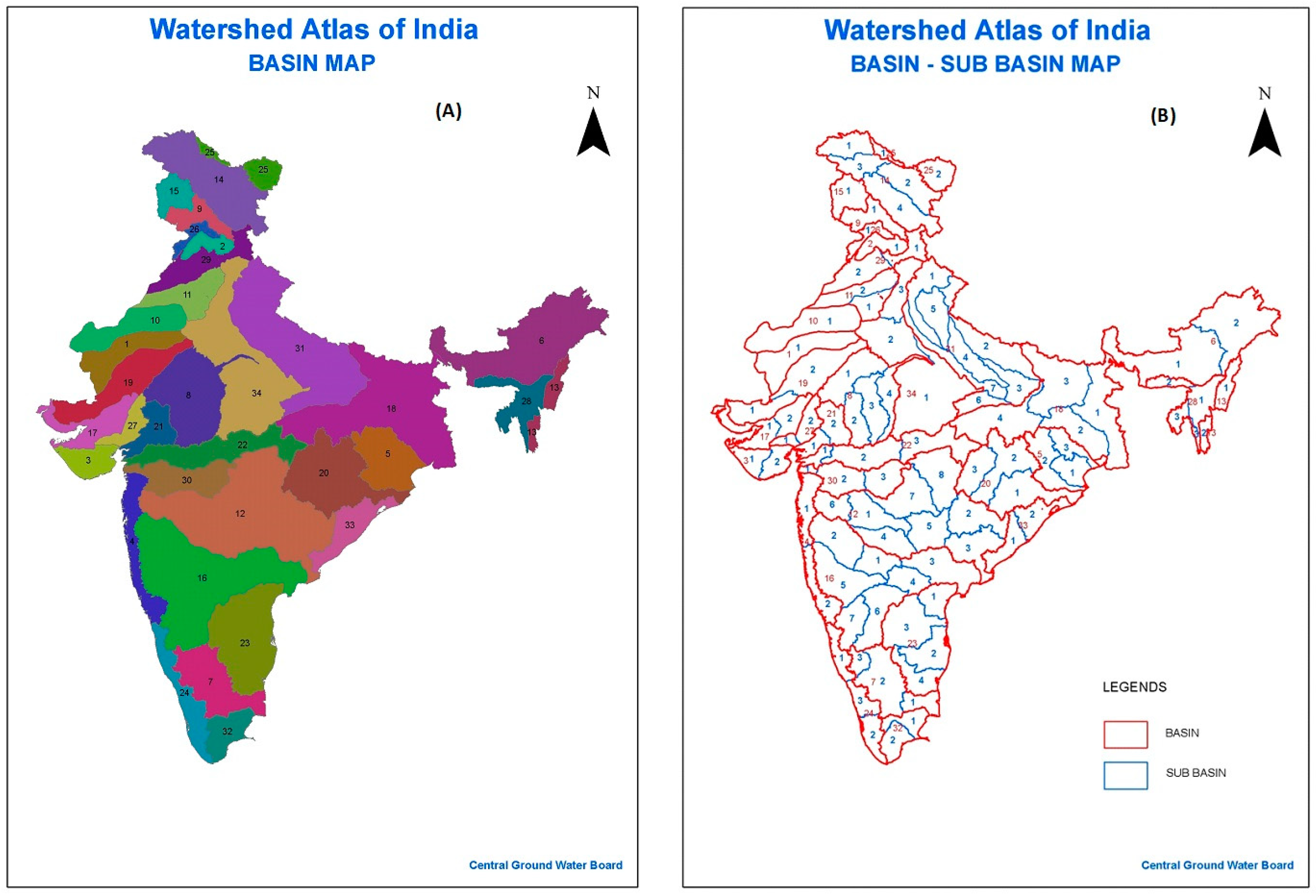
| Basin | Sub-Basin |
|---|---|
| 1. Barmer | The sand dunes of Barmer |
| 2. Beas | Beas |
| 3. Bhadar | Bhadar and other west-flowing rivers; Shetrunji and other east-flowing rivers |
| 4. Bhatsol (Rivers from Sheravatito Tapi flowing into the Arabian Sea) | Bhatsol and others; Vasishti and others |
| 5. Brahmani (from Mahanadi to Damodar) | Baitarni, Brahmani, and Subarnarekha |
| 6. Brahmputra | Downstream of confluence with the Subansirito–Bangladesh Border (Lower Brahmaputra); upstream of confluence with the Subansiri (Upper Brahmaputra) |
| 7. Cauvery | Lower Cauvery, Middle Cauvery, and Upper Cauvery |
| 8. Chambal | Banas, Chambal upstream of Maharana Pratap Sagar (Upper Chambal), Kali Sindh and others up to confluence with Parbati, and Parbati and others (Lower Chambal) |
| 9. Chenab | Chenab |
| 10. Churu | Ephemeral streams of Churu |
| 11. Ghaghar | Chautang and others; Ghagar and others |
| 12. Godavari | Between Gaikwad and Pochampad (Middle Godavari), Indravati, Kolab and others (Lower Godavari), Manjra, Pranhita and others, upstream of Gaikwad (Upper Godavari), Wardha, and Weinganga |
| 13. Imphal | Imphal and others, Mangpui Lui and others |
| 14. Indus | Gilgit, Shyok, up to confluence with Shyok (Indus Lower), and upstream of Shyok confluence (Upper Indus) |
| 15. Jhelum | Jhelum |
| 16. Krishna | Lower Bhima, Upper Bhima, Lower Krishna, Middle Krishna, Upper Krishna, Lower Tungabhadra, and Upper Tungabhadra |
| 17. Kutch | Drainage of Rann; Saraswati |
| 18. Lower Ganga | Bhagirathi and others (Lower Ganga), Damodar, Gandakand others, and Sone |
| 19. Luni | Lower Luni; Upper Luni |
| 20. Mahanadi | Lower Mahanadi, Middle Mahanadi, and Upper Mahanadi |
| 21. Mahi | Lower Mahi; Upper Mahi |
| 22. Narmada | Lower Narmada, Middle Narmada, and Upper Narmada |
| 23. Pennar (Cauvery To Krishna) | Musi and others, Palar and others, Pennar and others, and Ponnaiyar and others |
| 24. Periyar (Rivers from Kanyakumari To Sharavati Flowing into Arabian Sea) | Netravati and others, Periyar and others, and Varrar and others |
| 25. Qura-Qush | Shaksgam; Sulmar |
| 26. Ravi | Ravi |
| 27. Sabarmati | Lower Sabarmati; Upper Sabarmati |
| 28. Surma (Drainage Flowing into Bangladesh) | Barak, Kynchiang, and other south-flowing rivers; Naoch Chara and others |
| 29. Sutlej | Sutlej above Bhakra Dam (Upper Sutlej); Sutlej below Bhakra Dam (Lower Sutlej) |
| 30. Tapi | Lower Tapi, Middle Tapi, and Upper Tapi |
| 31. Upper Ganga | Above Ramganga confluence, Ghaghara, Ghaghara confluence to Gomti confluence, Gomti, Ramganga, Tons, and upstream of Gomti confluence to Muzaffarnagar |
| 32. Vaippar (Kanyakumari to Cauvery) | Pamba and others; Vaippar and others |
| 33. Vamsadhara (Godavari to Mahanadi) | Nagvati and others; Vamsadhara and others |
| 34. Yamuna | Confluence with Ganga to confluence with Chambal (Lower Yamuna), confluence with Chambal to confluence with Hindon (Middle Yamuna), and upstream of confluence with Hindon (Upper Yamuna) |
| References | Applications of the SWAT Model | SWAT Output Variables | Simulation Year/Model Used (Historical) |
|---|---|---|---|
| Singh and Saravanan (2022) [127] | Wunna watershed, India | Combination of stream flow and soil moisture simulation | Historical period 1998–2016 |
| Singh and Saravanan (2022) [128] | Three watersheds: Wunna, Bharathpuzha, and Mahanadi | Runoff and sediment | Historical period 2001–2016 |
| Singh and Saravanan (2022) [129] | Bharathpuzha catchment, India | Streamflow | Historical period 1998–2016 |
| Santra Mitra et al. (2021) [130] | Kangshabati River Basin of West Bengal | Runoff | Historical period 1982–2017 |
| Swain et al. (2021) [131] | Brahmani and Baitarani River catchments | Streamflow | Historical period 1979–2018 |
| Nune et al. (2021) [132] | Himayat Sagar (HS) catchment, India | Streamflow and groundwater levels | Historical period 1980–2007 |
| Horan et al. (2021) [133] | Cauvery catchment | Streamflow | Historical period 1986–2003 |
| Desai et al. (2021) [134] | Betwa River Basin | Streamflow | Historical period 2000–2011 |
| Joseph et al. (2021) [135] | Son River | Flow regimes | Historical period June 1971 to 1975 |
| Swain et al. (2020) [136] | Brahmani–Baitarani River Basin | Streamflow | Historical period 1990–2009 |
| Patil and Nataraja (2020) [137] | Hiranyakeshi watershed | Runoff | Historical period 1996–2015 |
| Shukla et al. (2020) [138] | Upper Ganga River Basin | Hydrological components | Historical period 1980 to 2012 |
| Setti et al. (2020) [139] | Nagavalli River Basin | Streamflow | Historical period 1970–2012 |
| Venkatesh et al. (2020) [140] | Tungabhadra River | Streamflow | Historical period 2002–2012 |
| Padhiary et al. (2020) [141] | Baitarani River Basin | Streamflow | Historical period 2021–2095 |
| Chauhan et al. (2020) [142] | Ghaggar River Basin | Streamflow | Historical period 1985–2015 |
| Singh and Saravanan (2020) [143] | Ib River watershed in Mahanadi River Basin | Streamflow | Historical period 1993 to 2011 |
| Kanishka and Eldho (2020) [144] | Godavari River Basin | Streamflow | Historical period 1995 to 2005 |
| Merina et al. (2019) [145] | Upper Girna sub-basin, Nashik, India | Streamflow; net inflow of the Girna dam | Historical period 2000–2015 |
| Visakh et al. (2019) [44] | Mahanadi River Basin, Brahmani–Baitarani River Basin, Hooghly River, and adjacent small river basins | Inter-comparison of water balance | Historical period 1987–2013 |
| Singh et al. (2019) [146] | Teesta river catchment, a part of North Sikkim, Eastern Himalayas, India | Water yield and streamflow | Historical period 1981–2005 |
| Budamala and Baburao Mahindrakar (2021) [147] | Kagna watershed of Krishna River Basin Telangana, India | Streamflow | Historical period 1987–2014 |
| Bhattacharya et al. (2019) [148] | Beas River Basin of North Western Himalaya | Streamflow and sediment yield | Historical period 1979–2016 |
| Paul et al. (2019) [149] | Baitarani River Basin, India | Streamflow simulation | Historical period 1977–2004 |
| Adhikary et al. (2019) [150] | Major river basins of southern India (the Pennar Basin of India) | Streamflow | Historical period 1992–2004 |
| Anshuman et al. (2019) [151] | Upper Godavari River Basin | Streamflow | Historical period 2000–2011 |
| Adla et al. (2019) [152] | Punpun River Basin | Streamflow | Historical period 1979–1997 |
| Ikhar et al. (2018) [153] | Jayakwadi reservoir stage I, Maharashtra, India | Inflows | Historical period 1981–2013 |
| Saini et al. (2018) [154] | Kanva watershed, a rural catchment in Kaveri Basin, Southern India | Water yield, groundwater recharge, percolation, and evapotranspiration | Historical period 1992–2016 |
| Tiwari et al. (2018) [155] | Satluj River Basin | Streamflow; runoff | Historical period 1982–2004 |
| Sinha and Eldho (2018) [156] | Netravati river basin in the Western Ghats of India | Monthly streamflow and sediment yield | Historical period 1979–2010 |
| Yaduvanshi et al. (2018) [157] | Subarnarekha River in India | Runoff response during extreme rain events | Historical period 1982–2011 |
| Goswami et al. (2018) [158] | Narmada River Basin | Estimation of surface runoff | Two active phases of JJAS 2016 |
| Anand et al. (2018) [38] | Ganga River Basin | Water balance due to change in land use | Historical period 1980–2013 |
| Nilawar and Waikar (2018) [41] | Purna River Basin, India | Climate and land-use changes on streamflow and sediment concentration | Historical period 1980–2005 |
| Chinnasamy et al. (2018) [40] | Ramganga Basin in India | Baseline hydrologic regime | Historical period 1999–2010 |
| Nagraj et al. (2018) [159] | Malaprabha sub-basin, a sub-basin in the Krishna River Basin | Streamflow | Historical period 1969–2005 |
| Shivhare et al. (2018) [160] | Part of the Ganga River Basin | Streamflow | Historical period 1996–2015 |
| Dutta and Sen (2018) [125] | Hirakud Reservoir, Mahanadi River | Soil erosion and sediment yield | Historical period 1990–2012 |
| Pati et al. (2018) [161] | Vansadhara River of the Mahanadi–Pennar Basin | Comparative analysis of the routing schemes | Historical period 2001–2012 |
| Yaduvanshi et al. (2018) [162] | Ghatshila catchment; middle-lower part of Subarnarekha River | Streamflow | Historical period 1982–2005 |
| Himanshu et al. (2018) [163] | Marol watershed, part of the Krishna River Basin | Runoff and sediment yield | Historical period 1998–2013 |
| Setti et al. (2018) [164] | Nagavali River Basin | Streamflow | Historical period 1985–2000 |
| Dutta et al. (2017) [124] | Tilaiya Reservoir, Jharkhand, India | Runoff and sediment yield | Historical period 1991–2000 |
| Hasan and Pradhanang (2017) [165] | Karnali River | Streamflow | Historical period 1979–2007 |
| Himanshu et al. (2017) [166] | Ken Basin, Central India | Runoff, sediment and water balance | Historical period 1982–2005 |
| Makwana and Tiwari (2017) [167] | Limkheda watershed, Gujarat, India | Streamflow modeling | Historical period 2007–2012 |
| Suryavanshi et al. (2017) [168] | Betwa River Basin, Central India | Water balance components | Historical period 1973–2001 |
| Jothiprakash et al. (2017) [169] | Musi River, a tributary of the Krishna River | Streamflow | Historical period 2001–2012 |
| Kumar et al. (2017) [118] | Tons River Basin | Streamflow | Historical period 1979 to 2011 |
| Halefom et al. (2017) [170] | Indore City, Madhya Pradesh, India | Water balance in the catchment | Historical period 1979 to 2013 |
| Kumar et al. (2017) [171] | Upper Kharun Catchment, Chhattisgarh, India | Land-use changes; water balance components | Historical period 1989–2011 |
| Abeysingha et al. (2016) [172] | Gomti River Basin of India | Production, evapotranspiration, and irrigation requirements | Historical period 1982–2010 |
| Alam et al. (2016) [173] | Brahmaputra River Basin | Estimation of future streamflow | Historical period 1981–2010 |
| Patel and Nandhakumar (2016) [174] | Anjana Khadi watershed, part of the Lower Tapi Basin | Estimation of runoff potential | Historical period 2006–2007 |
| Pandey et al. (2015) [116] | Mat River Basin | Streamflow | Historical periods 1988, 1991, and 1994 |
| Babar and Ramesh, (2015) [175] | Nethravathi River Basin | Streamflow | Historical period 2000–2009 |
| Abeysingha et al. (2015) [120] | Gomti River Basin in India | Water yield and evapotranspiration | Historical period 1985–2010 |
| Singh et al. (2015) [176] | Sutlej River sub-basin (middle catchment) | Streamflow and the water balance of the sub-basin | Historical period 1970–2010 |
| Uniyal et al. (2015) [177] | Upper Baitarani River Basin of Eastern India | Impact on water balance components | Historical period 1998–2005 |
| Reddy and Reddy (2015) [178] | Kaddam watershed, the central part of the middle Godavari | Estimation of runoff and sediment yield | Historical period 1996–2010 |
| Narsimlu et al. (2015) [179] | Kunwari River Basin, India | Estimation of streamflow | Historical period 1987–2005 |
| Pervez and Henebry (2015) [117] | Brahmaputra River Basin | Assessing freshwater availability | Historical period 1988–2004 |
| Verma and Jha (2015) [12] | Upper Baitarani River Basin, Eastern India | Streamflow and sediment yield | Historical period 1998–2005 |
| Chandra et al. (2014) [115] | Upper Tapi Basin | Estimation of runoff and sediment yield | Historical period 1976–2005 |
| Singh et al. (2014) [121] | Nagwa watershed in Jharkhand, India | Estimation of sediment yield | Historical period 1991–2007 |
| Murty et al. (2014) [119] | Ken Basin, Central India | Estimation of water balance | Historical period 1985–2009 |
| Reshmidevi and Nagesh Kumar (2014) [180] | Malaprabha River, North Karnataka, India | Streamflow | Historical period 1992–2003 |
| Wagner et al. (2013) [181] | Mula and Mutha Rivers’ catchment upstream of Pune | Estimation of water balance | Historical period from 1989/1990 to 2009/2010 |
| Santra and Das (2013) [123] | Watershed of the western catchment of Chilika Lake, India | Estimation of runoff | Historical period 1996–2006 |
| Singh et al. (2013) [182] | Tungabhadra River | Estimation of streamflow | Historical period 1990–2002 |
| Kushwaha and Jain (2013) [183] | Dabka watershed, Kumaon region Uttarakhand, India | Estimation of runoff | Historical January 2005–May 2007 |
| Bhuvaneswari et al. (2013) [113] | Cauvery River Basin | Streamflow and rice productivity | Historical period 1970–2008 |
| Garg et al. (2012) [184] | Upper Bhima River Basin | Agricultural water productivity | Historical period 1998–2005 |
| Garg et al. (2012) [185] | Kothapally watershed, Southern India | Surface runoff, evapotranspiration, and agricultural water | Historical period 1978–2008 |
| Perrin et al. (2012) [186] | Gajwel experimental watershed, India | Runoff and surface water storage; groundwater table fluctuations | Historical period 2000–2010 |
| Singh et al. (2012) [122] | Nagwa watershed | Sediment yield | Historical period 1993–2007 |
| References | Applications of the SWAT Model | SWAT Output Variables | Simulation Year/Model Used (Historical and Future) |
| Pandey et al. (2021) [187] | Upper Narmada Basin, India | Water balance | Historical period (1978 to 2005); future period (2011–2100) |
| Desai et al. (2021) [188] | Betwa River Basin | Water balance | Historical period (1961–1990); future periods (2010–2039, 2040–2069, and 2070–2099) |
| Thomas et al. (2021) [189] | Upper Narmada Basin | Streamflow | Historical period (1970–2005); future periods (2006–2040 (near-term), 2041–2070 (mid-term), and 2071–2099 (end-term)) |
| Alam et al. (2021) [190] | Brahmaputra River Basin | Streamflow | Historical period (1981–2010); future periods (2011–2040, 2041–2070, and 2071–2100) |
| Das et al. (2021) [191] | Gomti River Basin | Water yield and surface runoff | Historical period (2002–2013), future period ((2017–2039), mid-century period (2040–2069), and end century (2070–2099)) |
| Dash et al. (2021) [192] | Brahmani River Basin | Streamflow | Historical period (1970–1999); future period (2050) |
| Gaur et al. (2021) [193] | Subarnarekha Basin | Streamflow | Historical period (1981–2005); future period (2006–2049) |
| Abeysingha et al. (2020) [194] | Gomti River Basin | Flow regimes | Historical period (1982–2010); future periods (2020s, 2050s, and 2080s) |
| Sowjanya et al. (2020) [106] | Wardha watershed, India | Streamflow | Historical period (1975–2003); future period (2020–2099) |
| Sinha et al. (2023) [195] | Kadalundi River Basin, Western Ghats, India | Streamflow | Historical period (1981–2010); near (2011−2040), middle (2041−2070), and far (2071−2099) future periods |
| Nilawar and Waikar (2019) [84] | Purna River Basin, India | Streamflow and sediment concentration | Future periods P1 (2009–2031), P2 (2032–2053), P3 (2054–2075), and P4 (2076–2099) |
| Pandey and Palmate (2019) [126] | Betwa River Basin | Water yield and sediment yields | Baseline (1986–2005); future horizons (2020–2039, 2040–2059, 2060–2079, and 2080–2099) |
| Pandey et al. (2019) [83] | Upper Narmada Basin (UNB) | Water yield | Historical period (1970–2005); future period (2006–2100) |
| Chanapathi et al. (2018) [39] | Krishna River Basin | Rainfall extremes and water yield analysis | Historical period (1970–2005); future period (2006–2100) |
| Saharia and Sarma (2018) [82] | Bharalu (urban basin) and Basistha (rural basin) River Basins near the Brahmaputra River, India | Evaluate streamflow and water balance components variation | Historical period (1988 to 2012) and future periods (2046–2064 and 2081–2100) |
| Islam et al. (2018) [112] | Brahmaputra River Basin | Streamflow | Historical period (1980–2009); future periods in the 2020s (2010–2039), 2050s (2040–2069), and 2080s (2070–2099) |
| Saraf and Regulwar (2018) [196] | Upper Godavari River Basin, Maharashtra State, India | Runoff | Historical period (1985–2010); future periods (2011–2040 (2020s), 2041–2070 (2050s), and 2071–2099 (2080s)) |
| Sahoo et al. (2018) [197] | Gandherswari River Basin, West Bengal, India | Streamflow | Historical period (1990–2016), future GCM (2030, 2050, and 2080) of the HadCM3 A2 and B2 scenarios |
| Kumar et al. (2018) [198] | Tons River Basin Madhya Pradesh, India | LULC changes on Hydrol. Process. | Historical period from 1985 to 2015 and future period from 2015 to 2035 |
| Pandey et al. (2017) [199] | Armur watershed in Godavari River Basin, India | Estimate the water balance components | Baseline (1961–1990); future period (2071–2100); HadRM3 for the A2 and B2 scenarios |
| Kundu et al. (2017) [110] | Narmada River Basin, Madhya Pradesh, India | Water balance | Historical period (1961 to 2001); future periods in the 2020s (2011–2040), 2050s (2041–2070), and 2080s (2071–2099) |
| Singh and Goyal (2017) [111] | Teesta River catchment | Streamflow and water yield | Historical period (1980–2005); future periods (2011–2040, 2041–2070, and 2071–2100) |
| Mudbhatkal et al. (2017) [200] | Malaprabha River catchment and Netravathi River catchment | Streamflow | Historical period (1975–2004) and future period (2006–2070) |
| Singh and Goyal (2017) [201] | Teesta and Lachung Rivers | Streamflow, water depth, and precipitation | Historical period (1991–2005) and future period (2008–2100) |
| Mittal et al. (2016) [202] | Kangsabati River Basin | Flow regime | Historical period (1970–2008) and future period (2021–2050) |
| Kulkarni et al. (2014) [203] | Krishna River Basin | Surface flow, water yield, and ET and PET | Historical period (1961–1990); future periods in the 2020s (2011–2040), 2050s (2041–2070), and 2080s (2071–2098) |
| Mittal et al. (2014) [204] | Kangsabati River Basin | Flow regime | Historical periods (1970–1999 and 1989–2008); future period 2021–2050; and ECHAM5 and HadCM3 under the SRES A1B scenario |
| Narsimlu et al. (2013) [114] | Upper Sind River Basin, India | Estimate of the streamflow | Historical period (1961–1990), future period (2021–2050), and the end of the century (2071–2098) |
| Narula and Gosain (2013) [205] | Upper Yamuna watershed, North India | Streamflow, groundwater recharge, and nitrate load distributions in various components of the runoff | Historical period (1961–1990); future periods (2071–2100 and 2071–2098) |
| Study | SWAT-CUP Calibration and Validation Parameters | Statistical Parameters (Calibration/Validation) | SWAT Performance (Calibration/Validation) | Sensitivity Parameters (Rank) |
|---|---|---|---|---|
| Singh and Saravanan (2022) [127] | CH_N2, CN2, SOL_AWC, SOL_K, SOL_Z, ALPHA_BF, RCHRG_DP, REVAPMN, and SOL_BD | NSE; PBIAS | Satisfactory/very good | CN2; ALPHA_BF |
| Singh and Saravanan (2022) [128] | Wunna watershed, ALPHA_BF, CN2, CH_N2, SOL_BD SOL_Z, SOL_AWC, and CH_K2 and CANMX. Bharathpuzha, CN2, ALPHA_BF, SOL_BD, ESCO, REVAPMN, SOL_K, CH_N2, and CH_K2, GW_DELAY. Mahanadi, ALPHA_BF, CN2, SOL_BD, and GW_DELAY and SOL_K. | NSE; R2 | Very good/Good | CN2, ALPHA_BF, and SOL_BD |
| Singh and Saravanan (2022) [129] | SOL_AWC, CANMX, CH_K2, RCHRG_DP, CH_N2, GW_DELAY, CN2, SURLAG, SOL_BD, REVAPMN, SOL_Z, ALPHA_BF, EPCO, ESCO, GW_REVAP, and SOL_K | R2, NSE, PBIAS, and KGE | Good | SOL_AWC |
| Pandey et al. (2021) [187] | CN2, ALPHA_BF, and GQ_DELAY, EPCO, ESCO | R2; NSE | Good/Very good | CN2, ALPHA_BF, and GQ_DELAY |
| Santra Mitra et al. (2021) [130] | SOL_AWC, CH_N2, GW_DELAY, CN2, REVAPMN, ALPHA_BF, ESCO, GW_REVAP, and GWQMN | R2; NSE | Satisfactory | CN2 |
| Thomas et al. (2021) [189] | CN2, GWDELAY, GW_REVAP, GWQMN, SOL_AWC, and ALPHA_BF and ESCO | NSE, RMSE, RSR, and PBIAS and R2 | Good/Very good | CN2 |
| Swain et al. (2021) [131] | ALPHA_BF, ALPHA_BNK, CN2, CH_K2, CH_N2, GW_DELAY, GWQMN, GW_REVAP, REVAPMN, and SOL_AWC | NSE, PBIAS, and R2 | Satisfactory | ALPHA_BF |
| Nune et al. (2021) [132] | SOL_AWC, SOL_K, CN, STRUCTURES_K, RESERVOIRS_K, ALPHA_BH, GW_DELAY, ESCO, and SOL_BD | NSE and R2 | Good | Not Mentioned |
| Das et al. (2021) [191] | CN2, SOL_K, SOL_AWC, RCHRG_DP, SURLAG, REVAPMN, DEEPST, SOL_ALB, GWQMIN, GW_DELAY, ALPHA_BF, CANMX, and SOL_BD | NSE, PBIAS and R2 | Good | CN2 |
| Horan et al. (2021) [133] | SOL_BD, SOL_AWC, SOL_Z, SOL_K, CN2, GW_REVAP, REVAP_MN, GWQMN, GW_DELAY, SURLAG, ALPHA_BF, RES_K, and RES_K | NSE, PBIAS, and KGE | Good | Not Mentioned |
| Desai et al. (2021) [188] | CN2, SOL_AWC, GW_DELAY, REVAPMN, ESCO, GW_REVAP, GWQMN, CH_K2, ALPHA_BF, and EPCO | R2, NSE, RSR, and PBIAS | Very good/Satisfactory | CN2 |
| Dash et al. (2021) [192] | RCHRG_DP, SOL_K, CH_N2, SOL_AWC, ALPHA_BF, SLSUBBSN, ALPHA_BNK, GW_SPYLD, GW_DELAY, and GWQMN | R2, NSE, and PBIAS | Good | RCHRG_DP |
| Gaur et al. (2021) [193] | CN2, SOL_K, GW_REVAP, CH_N2, GW_DELAY, ALPHA_BF, ESCO, GWQNM | R2, NSE, and PBIAS | Satisfactory | CN2 |
| Joseph et al. (2021) [135] | CN2, AWC, Soil K, and ESCO | R2 | Good | CN2 |
| Alam et al. (2021) [190] | SOL_AWC, ALPHA_BF, GW_DELAY, GW_REVAP, CN2, SMTMP, ESCO, GWQMN, and REVAPMN | R2, NSE, P-factor, and R-factor | Very good | SOL_AWC |
| Swain et al. (2020) [136] | CN2, GW_DELAY, ALPHA_BF, GWQMN, CH_K2, CH_N2, ALPHA_BNK, SOL_AWC, REVAPMN, and GW_REVAP | R2, NSE, and PBIAS | Good | CN2; SOL_AWC |
| Patil and Nataraja (2020) [137] | CN2, SOL_AWC, ESCO, GW_DELAY, ALPHA_BF, GW_REVAP, and RECHRG_DP | R2; NSE | Satisfactory | CN2 |
| Shukla et al. (2020) [138] | CN_2, TLAPS, SOL_AWC, SOL_K, ALPHA_BF, GW_DELAY, ESCO, SMTMP, SMFMN, SMFMX, SNO50COV, SFTMP, TIMP, and SNOCOVMX | R2, NSE, and PBIAS | Very good | CN2 |
| Setti et al. (2020) [139] | HRU_SLP, LAT_TTIME, ALPHA_BNK, CH_K2, SLSUBBSN, ESCO, CN2, SOL_AWC, EPCO, OV_N, RCHRG_DP, SOL_K, GW_REVAP, GW_DELAY, ALPHA_BF, REVAPMN, GWQMN, SURLAG | NSE; PBIAS | Good | CN2 |
| Venkatesh et al. (2020) [140] | CN2, ALPHA_BF, GW_DELAY, GWQMN, CH_N2, CH_K2, SOL_AWC, SOL_K, ESCO, GW_REVAP, REVAPMN, SLSUBBSN, SLSOIL, and ALPHA_BNK | R2, NSE, and PBIAS | Good | CN2 |
| Padhiary et al. (2020) [141] | CN2, ALPHA_BF, GW_DELAY, GWQMN, CH_N2, CH_K2, SOL_AWC, SOL_K, ESCO, and SURLAG | R2, NSE, and PBIAS | Good | ALPHA_BF |
| Chauhan et al. (2020) [142] | CN2, ESCO, GWQMN, ALPHA_BF, GW_REVAP, GW_DELAY, SOL_K, and OV_N | R2, NSE, and PBIAS | Satisfactory | CN2 |
| Singh and Saravanan (2020) [143] | ALPHA_BF, CN2, CH_N2, CH_K2, RCHRG_DP, SOL_AWC, SOL_K, SOL_Z, SOL_BD, GW_DELAY, REVAPMN, ESCO, GWQMN, GW_REVAP, CANMX, EPCO, and SURLAG | R2, NSE, and PBIAS | Good | ALPHA_BF |
| Abeysingha et al. (2020) [194] | EPCO, ALPHA_BF, SURLAG, CH_N2, SOL_AWC, GWQMN, SOL_K, ESCO, CN2, CH_K2, RCHRG_DP, CANMX, POT_VOLX, OV_N, SOL_BD, POT_FR, and GW_DELAY | NSE, R2, PBIAS, and RSR | Good | CN2 |
| Sinha et al. (2023) [195] | SOL_AWC, SURLAG, CN2, ESCO, EPCO, ALPHA_BF, GW_DELAY, GW_REVAP, GWQMN, and RCHRG_DP | R2, NSE, and PBIAS | Good | CN2 |
| Kanishka and Eldho (2020) [144] | CN2, SOL_AWC, ESCO, SLSUBBSN, OV_N, HRU_SLP, GW_REVAP, GWQMN, and REVAPMN | R2, NSE, PBIAS | Good | CN2 |
| Sowjanya et al. (2020) [106] | CN2, ALPHA_BF, GW_DELAY, GWQMN, GW_REVAP, ESCO, SOL_K, ALPHA_BNK, SOL_AWC, REVAPMN, SOL_BD, OV_N, CH_K2, EPCO, HRU_SLP, CH_N2, and SLSUBBSN | R2; NSE | Very Good/Good | CN2 |
| Merina et al. (2019) [145] | CN, ALPHA_BF, GW_DELAY, GWQMN, GW_REVAP, REVAPMN, ESCO, CH_K2, SOL_AWC, SOL_K, SLSUBBSN, and CH_N2 | NS; R2 | Good/Good | ALPHA_BF |
| Nilawar and Waikar (2019) [84] | CN2, ALPHA_BF, GW_DELAY, GWQMN, GW_REVAP, ESCO, CH_N2, CH_K2, ALPHA_BNK, SOL_AWC, SOL_K, SOL_BD, USLE_C.plant, CH_COV2, USLE_K, LAT_SED, CH_COV1, SPCON, and SPEXP | R2; NSE | Very Good/Very Good | ALPHA_BNK |
| Visakh et al. (2019) [44] | ALPHA_BF, CH_K2, CN2, SURLAG, ESCO, GW_DELAY, SOL_AWC, GW_REVAP, REVAPMN, GWQMN, and SLSUBBSN | NSE | Good/Good | CN2 |
| Singh et al. (2019) [146] | CN2, ALPHA_BF, GW_DELAY, GWQMN, ESCO, SFTMP, SOL_AWC, SOL_K, CH_N2, CH_K2, ALPHA_BNK, SNOCOVMX, SNOCOVMN, SNO50COV, and PLR | R, R2, and RMSE | Good/Good | CN2 |
| Budamala and Baburao Mahindrakar (2021) [147] | CN2, EPCO, SOL_AWC, GW_REVAP, REVAPMN, GWQMN, GW_DELAY, ALPHA_BF, RCHRG_DP, and CH_K2 | NSE, PBIAS, R2 | Very Good/Very Good | CN2 |
| Bhattacharya et al. (2019) [148] | CN2, ESCO, SOL_AWC, ALPHA_BF, SURLAG, SOL_BD, ESCO, EPCO, TIMP, SFTMP, USLE_K, USLE_P, SPCON, SPEXP, ADJ_PKR | NSE; R2 | Satisfactory/Satisfactory | CN2 |
| Paul et al. (2019) [149] | CN2, GWQMN, GW_DELAY, ALPHA_BF, CH_N2, CH_K2, and ESCO | NSE, PBIAS, and R2 | Satisfactory/Satisfactory | CN2 |
| Adhikary et al. (2019) [150] | CN2, ESCO, GW_DELAY, SOL_AWC, RCHRG_DP, GW_REVAP, SOL_K, GWQMN, SOL_BD, ALPHA_BNK, ALPHA_BF, SLSUBBSN, EPCO, REVAPMN, and OV_N | R2, NSE, RSR, and PBIAS | Good/Very Good | CN2 |
| Anshuman et al. (2019) [151] | CN2, SOL_AWC, SOL_K, SOL_CLAY, ESCO, SLSUBBSN, HRU_SLP, GWQMN, REVAPMN, GW_REVAP, ALPHA_BF, RCHRG_DP, ALPHA_BNK, CH_K2, and CH_N2 | R2, NSE, and PBIAS | Very Good/Very Good | CN2 |
| Pandey and Palmate (2019) [126] | CN2, SURLAG, ALPHA_BF, GDRAIN, RCHRG_DP, ESCO, GWQMN, GW_DELAY, SOL_AWC, USLE_K, CH_ERODMO, RES_STLR_CO, PRF, CH_COV1, ADJ_PKR, RES_SED, CH_COV2, USLE_P, LAT_SED, USLE_C, AGRL, RES_NSED, SPEXP, and USLE_C | R2, NSE, and PBIAS | Good/good | CN2 |
| Adla et al. (2019) [152] | CH_K2, GW_DELAY, SOL_AWC, GW_REVAP, ESCO, CN2, ALPHA_BF, and SURLAG | P-factor, R-factor, R2, and NSE | Good/good | Not mentioned |
| Pandey et al. (2019) [83] | CN2, ALPHA_BF, GW_DELAY, GWQMN, ESCO, EPCO, GW_REVAP, REVAPMN, SOL_K, OV_N, SOL_AWC, CANMX, CH_N2, and HRU_SLP | R2; NSE | Good/Satisfactory | CN2 |
| Ikhar et al. (2018) [153] | CN2, ESCO, ALPHA_BF, GW_DELAY, SOIL_AWC, GWQMN, and GW_REVAP | NS, R2, and RSR | Very Good/Very Good | CN2 |
| Saharia and Sarma (2018) [82] | CN2, ALPHA_BF, ESCO, BLA, SOL_AWC, CANMX, SOL_Z, GW_DELAY, GW_REVAP, SLOPE, NPERCO, BIOMIX, SHALLST_N, SOL_NO3, and SOL_ORGN | RMSE, PBIAS, NSE, R2 | Good/Good | CN2 |
| Anand et al. (2018) [38] | CN2, SURLAG, GWQMN, GW_DELAY, ALPHA_BF, GW_REVAP, ESCO, OV_N, SFTMP, SMTMP, PLAPS, TLAPS, SOL_AWC, SMFMN, and SMFMX | NSE, R2, PBIAS, and RSR | Very Good/Very Good | Not Mentioned |
| Chanapathi et al. (2018) [39] | CN2, RCHRG_DP, GWREVAP, SOL_K, GWDELAY, CH_K2, CH_N2, ALPHA_BNK, REVAPMN, ALPHA_BF, GWQMN, and ESCO | R2; NSE | Good/Good | CN2 |
| Nilawar and Waikar (2018) [41] | GWQMN, GW_REVAP, CN2, GW_DELAY, SOL_K, REVAPMN, ALPHA_BF, ESCO | R2; NSE | Good/Good | Not Mentioned |
| Sinha and Eldho (2018) [156] | CN2, USLE_P, SOL_AWC, USLE_K, ESCO, LAT_SED, EPCO, HRU_SLP, SUR_LAG, SLSUBBSN, ALPHA_BF, GW_DELAY, GW_REVAP, CH_N2, RCHRG_DP, CH_K2, GWQMN, CH_COV1, and CH_ERODMO | NS, R2, and PBIAS | Good/Good | CN2 |
| Saini et al. (2018) [154] | SOL_AWC, CN2, SOL_K, ALPHA_BF, GWQMN, GW_REVAP, REVAPMN, RCHARG_DP, ESCO, SOL_AWC, SURLAG, and OV_N | R2, NSE, RSR, and PBIAS | Very Good/Very Good | Not Mentioned |
| Tiwari et al. (2018) [155] | CN2, ALPHA_BF, GW_DELAY, GWQMN, SFTMP, SMTMP, SMFMX, SMFMN, TIMP, SNOCOVMX, MSK_CO1, MSK_CO2 | NS; R2 | Good/Satisfactory | CN2 |
| Islam et al. (2018) [112] | ALPHA_BF, ALPHA_BNL, CH_N2, CN2, EPCO, ESCO, GWQMN, GW_DELAY, GW_REVAP, HRU_SLP, OV_N, REVAPMN, SFTMP, SLUSUBBSN, SOL_AWC, SOL_BD, and SOL_K | R2, NSE, PBIAS, RMSE, and RSR | Good/Satisfactory | CN2 |
| Nagraj et al. (2018) [159] | CN2, ESCO, SOL_AWC, GW_DELAY, and ALFA_BF | R2; NSE | Good/Good | CN2 |
| Shivhare et al. (2018) [160] | GW_DELAY, SOL_K, ALPHA_BF, CH_N2, CH_K2, CN2, USLE_P, SOL_AWC, SURLAG, USLE_K | R2; NSE | Very Good/Very Good | CH_K2 |
| Saraf and Regulwar (2018) [196] | CN2, ALPHA_BF, GW_DELAY, GWQMN, GW_REVAP, ESCO, CH_N2, CH_K2, SOL_AWC, SOL_K, SURLAG, CANMX | R2; NSE | Good/Good | CH-K2 |
| Sahoo et al. (2018) [197] | CN2, GW_DELAY, ALPHA_BF, GWQMN, GW_REVAP, REVAPMN, SOL_AWC, ESCO, SOL_K, ALPHA_BNK, CH_K2, EPCO, HRU_SLP, CH_N2, OV_N, SLSUBBSN, SOL_BD, and SURLAG | R2, NSE, and PBIAS | Satisfactory/Satisfactory | RCHRG_DP, CN2 |
| Yaduvanshi et al. (2018) [162] | CN2, ALPHA_BF, GW_DELAY, GWQMN, GW_REVAP, ESCO, CH_N2, CH_K2, and SOL_K | R2; NSE | Good/Good | CN2 |
| Kumar et al. (2018) [198] | ALPHA_BF, SOL_K, ESCO, GW_DELAY, CH_K2, and SLSUBBSN | P and R factor, R2 NSE, RSR, and PBIAS | Good/Good | ALPHA_BF |
| Pati et al. (2018) [161] | SOL_BD, CN2, ALPHA_BF, GW_DELAY, GWQMN, SOL_K, SOL_AWC, LAT_TTIME, REVAPMN, SURLAG, CH_N2, ESCO, EPCO, CH_K2, GW_REVAP, and CANMX | R2, NSE, and MAPE | Very Good/Good | CH_N2 |
| Yaduvanshi et al. (2018) [157] | CN2, ALPHA_BF, GW_DELAY, SOL_AWC, and ESCO | NSE;, P and R factors | Good/Good | CN2 |
| Himanshu et al. (2018) [163] | ALPHA_BF, BIOMIX, CH_COV2, CH_K1, CH_K2, CH_N2, CH_S1, CN2, EPCO, ESCO, GW_DELAY, GWQMN, GW_REVAP, OV_N, RCHRG_DP, REVAPMN, SLSUBBSN, SOL_AWC, SURLAG, SOL_K, SURLAG, USLE_K, and USLE_P | NSE, PBIAS, and RSR | Very Good/Very Good | CH_N2 |
| Hasan and Pradhanang (2017) [165] | CN2, OV_N, ALPHA_BF, GW_DELAY, GWQMN, GW_REVAP, RG_DP, REVAPMN, CH_N2, ESCO, EPCO, TLAPS, SOL_AWC, SMTMP, SMFMX, SMFMN, SFTMP, TIMP, and SURLAG | R2, NSE, and PBIAS | Very Good/Very Good | GWQMN, |
| Setti et al. (2018) [164] | LAT_TTIME, HRU_SLP, CN2, SOL_AWC, ESCO, SLSUBBSN, RCHRG_DP, EPCO, GWQMN, REVAPMN, OV_N, GW_DELAY, ALPHA_BF, and GW_REVAP | R2, NSC, PBIAS, and RSR | Very Good/Very Good | LAT_TTIME |
| Kundu et al. (2017) [110] | CN2, ESCO, SOL_ Z, SOL_AWC, CANMX, GWQ_MN, REVAPMN, BLAI, EPCO, GW_REVAP, SURLAG, ALPHA_BF, SOL_K, SLOPE, GW_DELAY, BIOMIX, SOL_ALB, SLSUBBSN, CH_N2, CH_K2, TLAPS, TIMP, SMTMP, SMFMX, SMFMN, and SFTMP | R2, NSE, PBIAS, and RSR | Very Good/Very Good | CN2 |
| Singh and Goyal (2017) [111] | CN2, ALPHA_BF, GW_DELAY, GWQMN, ESCO, SFTMP, SOL_AWC, SOL_K, CH_N2, CH_K2, and ALPHA_BNK | R2; NSE | Good/Good | CN2 |
| Suryavanshi et al. (2017) [168] | CN2, ESCO, SOL_AWC, SOL_Z, REVAPMN, GWQMN, CH_K2, ALPHA_BF, EPCO, CH_N2, GW_DELAY, SURLAG, SOL_K, and GW_REVAP | NSE, R2, PBIAS, and RMSE | Very Good/Very Good | CN2 |
| Makwana and Tiwari (2017) [167] | Input parameters by (Arnold et al. 2012). ALPHA_BF, CH_K2, SURLAG, and GWQMN | R2, NSE, RMSE, and mean absolute error (MAE) | Satisfactory/Satisfactory | ALPHA_BF |
| Himanshu et al. (2017) [166] | ALPHA_BF, CH_N2, CH_K2, CN2, SURLAG, ESCO, SOL_Z, GW_DELAY, CANMX, SOL_AWC, GW_REVAP, SOL_K, REVAPMN, BLAI, GWQMN, SLSUBBSN, EPCO, SLOPE, SOL_ALB, BIOMIX, CH_EROD, SPEXP, RCHRG_DP, SPCON, CH_COV, USLE_C, USLE, and USLE_P | NSE, R2, PBIAS, and RMSE | Very Good/Good | SPCON |
| Kumar et al. (2017) [118] | CN2, ALPHA_BF, GWQMN, ESCO, CH_K2, CH_N2, REVAPMN, SOL_AWC, HRU_SLP, SOL_K, SOL_BD, SLSUBBSN, GW_REVAP, EPCO, GW_DELAY, SFTMP, ALPHA_BNK, SURLAG, and OV_N | R2, NSE, PBIAS, and RSR | Good/Good | ALPHA_BF |
| Pandey et al. (2017) [199] | CN2, ESCO, GWQMN, SOIL_AWC, SOIL_Z, ALPL_BF, GW_REVAP, BLAI, EPCO, CH_K2 | R2, ENS, and PE | Good/Good | CN2 |
| Mudbhatkal et al. (2017) [200] | CN2, SOL_K, SLOPE, SOL_AWC, ESCO, SOL_Z, CANMX, CH_K2, SURLAG, ALPHA_BF, EPCO, CH_N, GW_DELAY, GW_REVAP | R2; NSE | Good/Good | CN2 |
| Jothiprakash et al. (2017) [169] | CH_K2, CN2, OV_N, SURLAG, ESCO, RCHRG_DP, SOL_K, GW_DELAY, GWQMN, GW_REVAP, EPCO, ALPHA_BF, SOL_AWC, and SOL_BD | R2, NSE, MAE, and PBIAS | Satisfactory/Satisfactory | CH_K2 |
| Singh and Goyal (2017) [201] | CN2, GW_DELAY, SOL_K, HRU_SLP, and ALPHA_BF | R2; NSE | Very Good/Very Good | CN2 |
| Kumar et al. (2017) [171] | CN2, ALPHA_BF, GWQMN, ESCO, CH_K2, CH_N2, REVAPMN, SOL_AWC, HRU_SLP, SOL_K, SOL_BD, SLSUBBSN, GW_REVAP, EPCO, GW_DELAY, SFTMP, ALPHA, _BNK, and SURLAG, OV_N | P and R factor, R2, NSE, PBIAS, and RSR | Good/Good | ALPHA_BF |
| Dutta and Sen (2018) [125] | CN2, SURLAG, CH_N, ESCO, SLSUBBSN, GWQMN, EPCO, GW_REVAP, SOL_AWC, SOL_ALB, GW_DELAY, ALPHA_BF, REVAPMN, SOL_K, and TLAPS | R2, NSE, and RSR | Good/Good | CN2 |
| Kumar et al. (2017) [81] | SOL_Z, EPCO, GW_REVAP, SOL_BD, GWQMN, ALPHA_BF, RCHRG_DP, SURLAG, SOL_K, SOL_AWC, CH_K2, ESCO, GW_DELAY, and CN2 | R2; NSE | Very Good/Very Good | CN2 |
| Abeysingha et al. (2016) [172] | ALPHA_BF, SOL_AWC, EPCO, GW_DELAY, RCHRG_DP, GW_REVAP, ESCO, CN2, GWQMIN, REVAPMIN, SOL_K, OV_N, CANMAX, CH_K2, and SOL_BD | NSE, R2, RMSE (RSR), and PBIAS | Good/Good and Satisfactory/Satisfactory | ALPHA_BF |
| Mittal et al. (2016) [202] | ALPHA_BF, GW_DELAY, GWQMN, GW_REVAP, ESCO, CH_N2, CH_K2, CN2, SOL_AWC, SOL_K, and SOL_BD | PBIAS, NSE, and R2 | Good/Good | CN2 |
| Pandey et al. (2015) [116] | ALPHA_BF, GWQMN, ESCO, CH_N2, REVAPMN, and SOL_AWC | R2; NSE | Very Good/Very Good | ALPHA_BF |
| Narsimlu et al. (2015) [179] | CN2, ALPHA_BF, GWQMN, ESCO, CH_K2, CH_N2, REVAPMN, SOL_AWC, HRU_SLP, SOL_K, SOL_BD, SLSUBBSN, GW_REVAP, EPCO, GW_DELAY, SFTMP, ALPHA_BNK, and OV_N | NSE, R2, PBIAS, and RSR | Very Good/Good | ALPHA_BNK, ESCO |
| Uniyal et al. (2015) [177] | ALPHA_BF, CH_K2, ESCO, SOL_K, SOL_AWC, CN2, GW_DELAY, SURLAG, CH_N2, and GWQMN | R2, MAE, and NSE | Very Good/Very Good | SOL_AWC |
| Abeysingha et al. (2015) [120] | RCHRG_DP, SOL_AWC, SOL_K, GW_DELAY, EPCO, OV_N, ESCO, CN2, GW_REVAP, ALPHA_BF, GWQMIN, REVAPMIN, CANMAX, and CH_K2 | NSE, RSR, and PBIAS | Satisfactory/Satisfactory | Not Mentioned |
| Pervez and Henebry (2015) [117] | CN2, ESCO, ALPHA_BF, PLAPS, TLAPS, SLSUBBSN, GWQMN, REVAPMN, GW_REVAP, and EPCO | PBIAS, NSE, R2, and RMSE | Very Good/Very Good | CN2 |
| Babar and Ramesh (2015) [175] | ALPHA_BF, CANMX, CH_K2, CN_N2, CN2, ESCO, GWQMN, REVAPMN, GW_DELAY, SOL_K, and SURLAG | NSE, R2, and RMSE | Very Good/Very Good | ALPHA_BF |
| Verma and Jha (2015) [12] | ALPHA_BF, CH_N2, SURLAG, CN2, CH_K2, GWQMN, ESCO, GW_DELAY, SOL_K, SOL_AWC, SOL_Z, GW_REVAP, EPCO, REVAPMIN, CANMX, SOL_ALB, BLAI, and BIOMIX | NSE, RSR, PBIAS, and R2 | Good/Good | ALPHA_BF |
| Murty et al. (2014) [119] | CN, SOL_AWC, SOL_Z, ESCO, GWQMN, REVAPMN, BLAI, CANMX, CH_K2, EPCO, GW_REVAP, and SOL_K | R2, PBIAS, NSE, RSR, and d index | Very Good/Very Good | GWQMN |
| Chandra et al. (2014) [115] | ALPHA_BF, CANMAX, CH_K2, CH_N2, CN2, EPCO, ESCO, GW_DELAY, GW_REVAP, GWQMN, REVAPMN, SOL_ALB, SOL_AWC, SOL_K, SOL_Z, SURLAG, RCHRG_DP, LAT_TIME, MANNING’S, “N” VALUE FOR OVERLAND FLOW, SOL_BD, SPCON, CH_EROD, USLE_P, and USLE_C | NSE; RSR | Satisfactory/Satisfactory | Not Mentioned |
| Singh et al. (2014) [121] | USLE_P, CH_EROD, SPCON, CH_COV, SPEXP, USLE_C | R2, NSE, and PBIAS | Good/Good | USLE_P |
| Reshmidevi and Nagesh Kumar (2014) [180] | ALPHA_BF, CH_K2, CH_N2, CN2, EPCO, ESCO, GW_DELAY, GW_REVAP, GWQMN, RCHRG_DP, REVAPMN, SOL_AWC, SOL_K, and SURLAG | R2, NSE, and RMSE | Very Good/Very Good | RCHRG_DP |
| Kushwaha and Jain (2013) [183] | CN2, ESCO, SOL_Z, SOL_K, SOL_AWC, CH_N, GWDELAY, GW_REVAP, REVAPMN, GWQMN, ALPHA_BF, RCHRG_DP, and SURLAG | R2, NSE, and RMSE | Good/Good | CN2 |
| Singh et al. (2013) [182] | CN2, ALPHA_BF, GW_DELAY, GWQMN, GW_REVAP, ESCO, CH_N2, CH_K2, ALPHA_BNK, and SOL_K | R2; NSE | Good/Good | CH_K2 |
| Narsimlu et al. (2013) [114] | CN2, ALPHA_BF, GW_DELAY, GWQMN, GW_REVAP, ESCO, EPCO, CH_N2, CH_K2, ALPHA BNK, SOL_AWC, SOL_K, SOL_BD, and SFTMP | R2; NSE | Very Good/Very Good | SOL_AWC |
| Santra and Das (2013) [123] | ALPHA_BF, CH_K2, CH_N, CN2, ESCO, GW_DELAY, GWQMN, and SURLAG | NSE; RMSE | Good/Good | CH_K2 |
| Narula and Gosain (2013) [205] | SMTMP, SMFMX, SMFMN, TIMP, SFTMP, CN2, ESCO, AWC, SOL_K, CH_K2, GW_DELAY, and SURLAG | R2; NSE | Very Good/Very Good | TIMP |
| Garg et al. (2012) [184] | RCHRG_DP, CN2, ALPHA_BF, ESCO, SOL_AWC, SOL_Z, GW_DELAY, GW_REVAP, SURLAG, and REVAP_MN | R; NSE | Satisfactory/Satisfactory | RCHRG_DP |
| Singh et al. (2012) [122] | USLE_P, CH_EROD, SPCON, CH_COV, SPEXP, and USLE_C | R2; NSE | Good/Good | USLE_P |
Disclaimer/Publisher’s Note: The statements, opinions and data contained in all publications are solely those of the individual author(s) and contributor(s) and not of MDPI and/or the editor(s). MDPI and/or the editor(s) disclaim responsibility for any injury to people or property resulting from any ideas, methods, instructions or products referred to in the content. |
© 2023 by the authors. Licensee MDPI, Basel, Switzerland. This article is an open access article distributed under the terms and conditions of the Creative Commons Attribution (CC BY) license (https://creativecommons.org/licenses/by/4.0/).
Share and Cite
Dubey, S.K.; Kim, J.; Her, Y.; Sharma, D.; Jeong, H. Hydroclimatic Impact Assessment Using the SWAT Model in India—State of the Art Review. Sustainability 2023, 15, 15779. https://doi.org/10.3390/su152215779
Dubey SK, Kim J, Her Y, Sharma D, Jeong H. Hydroclimatic Impact Assessment Using the SWAT Model in India—State of the Art Review. Sustainability. 2023; 15(22):15779. https://doi.org/10.3390/su152215779
Chicago/Turabian StyleDubey, Swatantra Kumar, JungJin Kim, Younggu Her, Devesh Sharma, and Hanseok Jeong. 2023. "Hydroclimatic Impact Assessment Using the SWAT Model in India—State of the Art Review" Sustainability 15, no. 22: 15779. https://doi.org/10.3390/su152215779
APA StyleDubey, S. K., Kim, J., Her, Y., Sharma, D., & Jeong, H. (2023). Hydroclimatic Impact Assessment Using the SWAT Model in India—State of the Art Review. Sustainability, 15(22), 15779. https://doi.org/10.3390/su152215779