Numerical Simulation of 3D Flow Structure and Turbulence Characteristics near Permeable Spur Dike in Channels with Varying Sinuosities

Abstract

Owing to the different degrees of bending in rivers in nature, it is difficult to conduct experiments in situ. In this study, the renormalization group (RNG) k-ε turbulence model in ANSYS Fluent was used to analyze the three-dimensional flow structure and turbulence characteristics near a spur dike and to evaluate the variation trend of flow in rivers with different degrees of bending. The results show that in channels with different curvatures, the vortex appears between the spur dikes and is disturbed by the permeable hole, and the backflow area moves downstream. The strength of secondary flow (SSF) fluctuates greatly in the vicinity of the spur dike and the downstream region, and the peak value appears 3.22 m (21.5 times L) away from the inlet of the bend. The SSF increases as the bend curvature increases. The SSF displays similar variation trends in the three kinds of bends. The peak value of normalized turbulent kinetic energy (NTKE) appears 3.14 m away from the entrance of the bend, the NTKE is the largest in the 45° bend and the smallest in the 180° bend, and it decreases only at distances of 3.25–4.19 m away from the entrance of the bend as the bend curvature increases.

1. Introduction

Comparing the time-averaged flow fields in river channels with different curvatures helps us understand the variations in water flow with the curvature of the channel. This helps us assess hydraulic characteristics such as flow velocity, discharge, water surface elevation, and sediment transport. This is of significant importance for river management, channel modifications, and flood control. Additionally, the characteristics of time-averaged flow fields in channels with different curvatures assist hydraulic engineers in predicting velocity distribution and sediment transport, and they have value in the proper design of channel improvement structures. Furthermore, curvature variations can lead to significant flow instabilities in the channel, such as vortices and turbulence. Studying the flow field characteristics in channels with different curvatures helps us understand the development trends of flow in curved channels and aids in predicting channel bed deformation and channel erosion. Lastly, the turbulence and variations in flow velocity in curved channels can impact the habitats and migration patterns of aquatic organisms. Comparing the time-averaged flow fields in channels with different curvatures provides a basis for the preservation and restoration of river ecosystems. During the past few decades, hydraulic engineers have devoted considerable attention to the ecological restoration of rivers, as well as to restraining the deformation of river beds and preventing the uncontrolled migration of the outlines of rivers. The purpose of river regulation and river ecological restoration is to improve the stability of the river, improve water quality, increase biodiversity, and ensure a more suitable living environment for aquatic organisms [1]. Spur dikes are widely used by hydraulic engineers globally as river regulation structures. They are artificial structures that are connected to the river bank at one end and extend into the river at the other end [2]. Spur dikes change the direction of water flow, so as to reduce the erosion of river banks and prevent sediment deposition in local areas, which in turn helps achieve the goals of river regulation and ecological restoration. Spur dikes are classified into two types based on the materials used in their construction [3], namely impermeable and permeable spur dikes. Impermeable spur dikes are constructed using artificial impermeable materials like concrete and can be submerged or nonsubmerged spur dikes. These hydraulic structures are also called curved weirs or barbs. Impermeable spur dikes are characterized by flat tops and vertical sides [4,5]. Permeable spur dikes are constructed using permeable materials, such as gravel piles or wood; examples of such dikes include the new type of permeable spur dike recently proposed by Hu et al. [6]. For rivers requiring manual intervention, spur dikes or spur dike groups are typically constructed on one or both sides of the river [7]. Considerable academic attention has been devoted to impermeable spur dikes globally, with previous studies focusing on flow erosion, sediment deposition, spur dike layout spacing, spur dike geometric size, and other aspects. Rajaratnam and Nwachukwu [8] observed the scouring process near spur dikes in clear water in the laboratory using flumes, their results show that the scour hole depth was related to the scouring time, and the final morphology of the scour hole was similar under different working conditions. Przedwojski [9] also evaluated the scouring effect of the flow near spur dikes; his study used a two-dimensional numerical model to calculate streambed scour under steady-state conditions and proposed an equation to calculate the depth of the scour hole. Since then, numerous studies have evaluated flow erosion and sediment deposition near spur dikes [5,10,11,12,13]. Moreover, the geometric design and size, as well as the layout and spacing, of spur dikes have attracted the attention of hydraulic engineers. Ikeda et al. [14] observed a river channel and determined that the mass exchange rate between the mainstream and the obstacle was higher when the ratio of the spur dike spacing (D) to the spur dike length (L) was approximately 2–3. Fazli et al. [11] and Haghnazar et al. [15] found that the discharge and geometry of a spur dike are important factors affecting channel erosion. Their study found that increased flow in the channel will result in increased scour hole size and decreased sediment height, Froude number is directly related to scour depth, and a change in the length of the spur dike will directly affect the width of the recirculation zone behind the spur dike. Azamathulla et al. [16], Azamathulla and Yusoff [17], and Pandey et al. [18] inferred that the scouring depth of vertical breakwater primarily depends on the length of vertical breakwater, flow parameters, and sediment characteristics. Their study showed that smaller inhomogeneity of sediment mixtures will result in an increase in the size of the scour hole. Masjedi et al. [19] studied the relationship between scour time and scour hole size and found an empirical equation between scour hole depth and scour time. The regression coefficient was 0.97. Previous studies have also been conducted on permeable spur dikes, focusing on river regulation, scouring characteristics near spur dikes, riverbed shear stress, flow structure, permeability, and other aspects. Fukuoka et al. [20] and Li et al. [21] studied the scouring characteristics and bed shear stress near underwater obstacles and found that scouring does not easily occur in spur dikes with good permeability and that the bed shear stress is significantly reduced. By comparing the flow structure and scouring characteristics, Osman and Saeed [22] and Zhou et al. [23] found that permeable spur dikes could slow down channel scouring and reduce the size of scouring holes. Their findings also confirm that the stability, safety, and reliability of permeable spur dikes are better than those of traditional spur dikes. Later, other studies investigated the permeability rate. Elawady et al. [24] and Nath and Misra [25] found that an increase in permeability led to a decrease in scour hole size. Li and Altinakar [26] introduced the movable-bed physical model into their experiment and conducted a comparative study of spur dikes with different lengths and permeability rates. They found that the effect of flow scour on the stability of the spur dike was minimal when the ratio of the length of the spur dike to the width of the flume was 0.2 and the permeability rate was 30%. Permeable spur dikes primarily improve safety performance by reducing the stress concentration in the dam body through the installation of water-permeable holes or seepage orifices. Simultaneously, permeable spur dikes provide a suitable habitat for fish and other benthic organisms. Mostafa et al. [27] conducted a comparative analysis through flume tests to investigate the effects of permeable spur dikes and solid spur dikes on the main channel and water depth. They concluded that the water depth at the centerline of the main channel remains unchanged for the permeable spur dikes, while the solid spur dikes cause a change in water depth at the centerline of the main channel. Yun et al. [28] studied permeable spur dikes with permeability rates of 6.8%, 10.4%, 14.1%, 17.5%, and 22.5%. Under the same conditions of permeable hole size, they found a negative correlation between potential energy and void ratio in the upstream of the spur dikes. Under the same permeability rate conditions, there was a negative correlation between potential energy in the downstream, further away from the spur dikes, and void size. Fan et al. [29] discovered that the intensity of backflow behind spur dikes gradually weakened as the permeability rate increased. When the permeability rate reached 20%, the backflow intensity was already relatively weak. During the process of increasing the permeability rate from 20% to 30%, the length of the backflow zone behind the spur dikes remained relatively constant, while the width gradually decreased. When the permeability rate reached 40%, the backflow basically disappeared. To clearly observe the backflow zone behind the spur dikes and the variation in turbulent kinetic energy along the flow path, the chosen permeability rate in this study was not excessively high. Considering the aforementioned research, the final chosen permeability rate was 20%.

It is clear that several studies have focused on flow scouring and sediment deposition near improved permeable spur dikes or traditional impermeable spur dikes, and they have quantitatively measured the sediment deposition patterns and the scour hole sizes. However, the three-dimensional turbulent flow characteristics near spur dikes have not been fully considered in previous studies. Turbulent flow characteristics, as an important index to evaluate the flow pattern, play an extremely important role in both channel erosion and sediment deposition. The flow pattern, turbulent kinetic energy, and manner in which the secondary flow develops near the permeable spur dike need to be further studied, especially in channels with different sinuosities.

Particle image velocimetry (PIV) has been applied to scientific research since the 1980s, and hydraulic engineers have attempted to use PIV to measure the time-averaged flow field near spur dikes. PIV is a noncontact technique; so, the measuring device does not interfere with the flow field, and it can be used to accurately quantify the three instantaneous velocity components within the flow field [30]. Noncontact image analysis techniques such as PIV can measure the flow field in detail at the scale of turbulence [31] and can capture particle flow trajectories in the flow field. Moreto et al. [30] used PIV technology to quantitatively study the three-dimensional velocity field and pressure field. In their study, they measured flow velocities on multiple closely spaced parallel planes and reconstructed the pressure field to derive a water surface profile. Using PIV technology, You and Tinoco [32] conducted an indoor experiment in a circulating water flume to track the behavior of Stokes particles near underwater obstacles. They found that the flow structure formed near the barrier would provide favorable conditions for the migration of high concentrations of particulate matter. In a laboratory, He et al. [33] measured the vertical velocity with PIV, and they used the PIV technique in their study to calibrate the flume for measuring critical bed shear stress. PIV technology has also been used in flume experiments.

Owing to the size limitations of laboratory flumes and the difficulty in conducting these experiments, previous studies have not been able to determine the variation trends in flow patterns, turbulent kinetic energy, and secondary flow in rivers with different bending degrees after permeable spur dikes were constructed, although these factors are essential for exploring the characteristics of open-channel flow and maintaining the stability of open channels. For example, numerical simulations of the horseshoe vortex, shear layer vortex, and recirculation area near nonsubmerged spur dikes in open channels have been carried out in previous studies, but these studies have failed to determine the variation trend after time averaging [34,35,36,37,38,39]. These studies lacked a detailed comparison between the experimental values and simulated values in the three-dimensional velocity field. Through a numerical simulation study on the flow characteristics, vortex structure, and mass exchange near a single spur dike and multiple spur dikes using Large Eddy Simulation (LES), McCoy et al. [40,41,42] found that the vortex system tends to be complex, and the mass exchange rate increases under submerged conditions. The k-ε model has also been used to reproduce the local flow and sediment transport around impermeable spur dikes [43]. Thus, it is clear that the current understanding of the flow pattern, turbulent kinetic energy, secondary flow, and other time averages in channels with different bending degrees is limited.

In channels with different sinuosities, the flow field around spur dikes has obvious 3D flow characteristics. Software programs such as FLUENT 2019 R3are used to predict the flow structure and scour characteristics in open channels. Reynolds-Averaged Navier–Stokes (RANS) and LES are the most popular methods. Using the LES method to calculate turbulence characteristics yields good results, but it is computationally intensive. Recently, Haider et al. [44], Mulahasan et al. [45], Ouillon and Dartus [46], and Yazdi et al. [47] compared numerical modeling results with experimental results and concluded that the RANS method can be used to predict open-channel flow. The RANS model transforms the unsteady turbulence problem into a steady problem by time-averaging the N-S equations, and it solves the mean flow field. Through comprehensive consideration, the RANS model was adopted in this study. The commercial software FLUENT 2019 R3 was used to solve the RANS equations.

Rivers in nature exhibit different degrees of meandering, and therefore, according to previous research, the flow structure and turbulence characteristics obtained by experiments or simulations of rivers with only one kind of meandering degree cannot directly demonstrate the influence of the meandering degree of rivers. Therefore, the flow structure and turbulence characteristics of open channels with different bending degrees after setting permeable spur dikes are analyzed by combining physical experiments with numerical simulation. In this study, the measured velocity is compared with the numerical simulation velocity to verify the reliability of the numerical simulation results, and then the flow pattern, NTKE, and SSF around the permeable spur dikes are studied using numerical simulation for bends of 45°, 90°, and 180°. The curvatures of the three bends are 0.125, 0.25, and 0.5, respectively. This approach first ensures the reliability of turbulence models and then utilizes numerical simulations to study various curved channels, which compensates for the limitation of laboratory experiments in providing multiple types of curved channels. It effectively expands the scope of research, freeing it from being confined to only one type of curved channel. The objectives of this study are, first, to validate the RNG k-epsilon turbulence model and demonstrate its reliability and, secondly, to summarize the variations in time-averaged flow fields in three typical curved river channels and then predict the flow field variations in other types of curved channels. This will provide a reference for natural river management and river ecosystem restoration in the natural environment.

2. Model Introduction

2.1. Numerical Model Governing Equations

The assumptions in mathematical modeling include the following: 1. Reynolds averaging: Turbulence models are based on the concept of Reynolds averaging, which means that the physical quantities (velocity, pressure, etc.) in the flow field are divided into mean components and turbulent components, and turbulence is handled by averaging over time. 2. Shear stress transport: The model assumes that the turbulent kinetic energy and turbulent dissipation rate are mainly determined by the turbulence transport and dissipation caused by velocity shear. These two variables play different roles in different turbulent motions. 3. Turbulent energy transport: This model assumes that the transport of turbulent energy is controlled by the nonlinear convection of turbulent velocity and the diffusion caused by turbulent shear. 4. Turbulent dissipation rate transport: This model assumes that the turbulent dissipation rate is mainly determined by the transport of turbulent energy dissipation, turbulent dissipation caused by turbulent shear, and the transport of the turbulent dissipation rate itself. 5. Turbulent shear production: The model considers the generation of turbulent shear, which refers to the influence of velocity gradients on turbulent energy and turbulent dissipation rate. 6. Isotropy: The RNG k-ε model typically assumes that turbulence is isotropic, which means that the statistical characteristics of turbulence are similar in all directions. 7. Constant density and viscosity: This model usually assumes that the density and viscosity of the fluid are constants and do not vary with temperature or pressure.

The governing Reynolds-Averaged Navier–Stokes equations are as follows:

The continuity equation is used to describe the mass conservation of a fluid in space. It states that the mass flow rate of the fluid at any given time and spatial point is conserved, meaning that the mass inflow equals the outflow. The momentum equation, on the other hand, is used to describe the balance between the motion of the fluid and the forces acting on it. It describes the relationship between the velocity and pressure of the fluid at a given time and spatial point, where the rate of change in momentum equals the sum of the forces acting on the fluid. In turbulent flow, the purpose of the momentum equation is to reveal the mechanisms of turbulent flow generation and energy conversion, as well as to describe the interaction between vortical structures and fluid motion in turbulent flow.

Continuity equation and momentum equation:

$$\frac{\partial \rho }{\partial t}+\frac{\partial \rho u_i}{\partial x_i}=0,$$

(1)

$$\frac{\partial \left(\rho u_i\right)}{\partial t}+\frac{\partial }{\partial x_j}\left(\rho u_i{u}_j\right)=-\frac{\partial p}{\partial x_i}+\frac{\partial }{\partial x_j}\left[\mu \left(\frac{\partial u_i}{\partial x_j}+\frac{\partial u_j}{\partial x_i}-\frac{2}{3}{\delta }_{ij}\frac{\partial u_i}{\partial x_i}\right)\right]+\frac{\partial }{\partial x_j}\left(-\rho \overline{u_i^{\prime }{u}_j^{\prime }}\right)$$

(2)

where $u_i$ is the velocity component; $t$ is the time; $\rho$ is the density of fluid; $p$ is the mean pressure; $\mu$ is the dynamic viscosity; ${\delta }_{ij}$ is the Kronecker delta; and $-\rho \overline{u_i^{\prime }{u}_j^{\prime }}$ is called Reynolds stress;

$$-\rho \overline{u_i^{\prime }{u}_j^{\prime }}={\mu }_t\left(\frac{\partial u_i}{\partial x_j}+\frac{\partial u_j}{\partial x_i}\right)-\frac{2}{3}\left(\rho k+{\mu }_t\frac{\partial u_i}{\partial x_i}\right){\delta }_{ij}$$

(3)

where ${\mu }_t$ is turbulent viscosity and $k$ is turbulent kinetic energy.

2.1.1. RNG k-ε Model

The turbulent kinetic energy transport equation is used to describe the transport and change in turbulent kinetic energy in the flow field, and the purpose of this equation is to provide the physical laws of turbulent energy conversion and transport in order to more accurately simulate turbulent flow and predict the generation and evolution of turbulent eddies. The turbulent dissipation rate equation is used to describe the process of dissipation and decay of turbulent energy, and the purpose of this equation is to provide the mechanism that describes the loss of turbulent energy and the interaction between turbulent energy conversion and dissipation in turbulent flows.

Turbulent kinetic energy transport equation and turbulent kinetic energy dissipation rate ε equation:

$$\frac{\partial \left(\rho k\right)}{\partial t}+\frac{\partial \left(\rho k{u}_i\right)}{\partial x_i}=\frac{\partial }{\partial x_j}\left({\alpha }_k{\mu }_{eff}\frac{\partial k}{\partial x_j}\right)+G_k-\rho \epsilon ,$$

(4)

$$\frac{\partial \left(\rho \epsilon \right)}{\partial t}+\frac{\partial \left(\rho \epsilon u_i\right)}{\partial x_i}=\frac{\partial }{\partial x_j}\left({\alpha }_{\epsilon }{\mu }_{eff}\frac{\partial \epsilon }{\partial x_j}\right)+C_{1\epsilon }^{\ast }\frac{\epsilon }{k}{G}_k-C_{2\epsilon }\rho \frac{{\epsilon }^2}{k}$$

(5)

where $\epsilon$ is turbulent dissipation rate; ${\mu }_{eff}=\mu +{\mu }_t$, ${\mu }_t=\rho C_{\mu }{k}^2/\epsilon$, $C_{\mu }=0.0845$; ${\alpha }_k={\alpha }_{\epsilon }=1.39$; $G_k$ is the pressure generation term; $C_{1\epsilon }^{\ast }=C_{1\epsilon }-\eta \left(1-\eta /{\eta }_0\right)/1+\beta {\eta }^3$, $\eta =Sk/\epsilon$, $S={\left(2S_{ij}{S}_{ij}\right)}^{1/2}$, $S_{ij}=\frac{1}{2}\left(\frac{\partial u_j}{\partial x_i}+\frac{\partial u_i}{\partial x_j}\right)$, $C_{1\epsilon }=1.42$, ${\eta }_0=4.38$, $\beta =0.012$; $C_{2\epsilon }=1.68$.

2.1.2. Volume of Fluid (VOF) Model

The VOF model (Volume of Fluid model) is intended to be used to simulate the behavior and interaction of multiphase fluids such as liquids and gases. The model describes the motion and morphological changes at the fluid interface by tracking and calculating the volume fractions of the different phases. The main significance of the VOF model is that it can provide detailed information about the behavior of multiphase fluids and the ability to predict it. The model allows us to accurately simulate and predict phenomena such as interactions between different phases such as liquids and gases, the motion of interfaces, and the separation and aggregation of droplets.

The equation for dynamic tracking of the VOF is as follows:

$$\frac{\partial F}{\partial t}+u_i\frac{\partial F}{\partial x_i}=0,$$

(6)

Among

$$F=\frac{V_F}{V}$$

(7)

where $V_F$ is the volume of the fluid in the cell and $V$ is the volume of the cell. If $F=1$, the cell is completely filled with fluid; if $F=0$, the cell is empty and contains no fluid; and if $0<F<1$, there is a free surface in the cell.

2.2. Numerical Model

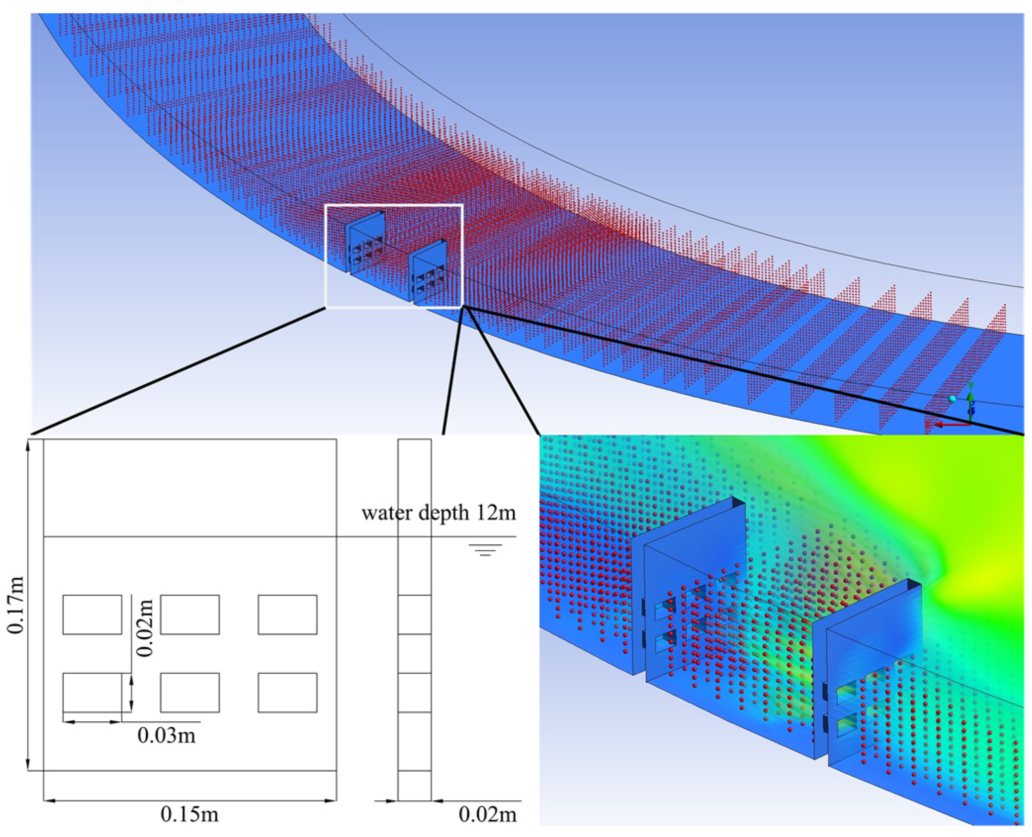
Figure 1 shows the schematic diagram of the computational field in the numerical model. For the purpose of comparing the variations in time-averaged flow fields in typical curved channels, after reviewing the existing research findings, we found that 90° and 180° bends have received considerable attention. This indicates that these two types of bends are representative. Therefore, for this study, we decided to choose 45°, 90°, and 180° bends in a decreasing order of curvature. The radii of the 45°, 90°, and 180° bends with different bending degrees are 2 m, 4 m, and 8 m, respectively. The upstream length of the laboratory flume and numerical model is 6.28 m, which is 42 times the length of the spur dike, allowing for sufficient development of the upstream flow. The width of the laboratory flume is 0.8 m, and for the validation of the model, the width of the numerical model is kept consistent with the physical model. Based on existing research, the ratio of the spur dike length to the flume width is around 0.2, and the ratio of the spur dike length to the water depth is around 1.5. Therefore, for this study, the ratio of the spur dike length to the flume width is set as 0.19, and the ratio of the spur dike length to the water depth is set as 1.25, ultimately determining the length, thickness, and height of the spur dike as 0.15 m, 0.02 m, and 0.17 m, respectively. Previous research has suggested an optimal permeability of 20% to 30%. Hence, this study adopts a permeability of 20%. The proportional parameters between the spur dike and the flume, as used in the experiment, are strictly determined according to recommended values from previous studies. Additionally, model validation was conducted in the initial stages of the research, ensuring that the spur dike and river align with the objectives and model of this study. The arrangement and details of the spur dikes are shown in Figure 2. The mesh is dense upstream and downstream of the spur dike, and the distribution of mesh nodes in the calculation field is adjusted. Finally, a set of meshes with a total number of 1.8 million, a maximum mesh size of 2 cm, and a quality greater than 0.9 is obtained.

In the FLUENT software, the flow inlet was defined as the velocity inlet; the top boundary of the numerical model was set to be the symmetry plane boundary; the riverbed, spur dike, and other positions were solid walls; enhanced walls were selected for near-wall treatment; and the tailgate was set to be a pressure outlet. The present study involves designing high-Reynolds-number water flow conditions in a curved channel. The medium turbulence intensity ranges from 5% to 10%, while the turbulence viscosity ratio is set between 10 and 100. Considering that the boundary conditions for the water tank in this study are not complex, with an inlet flow velocity of 0.52 m/s and a Reynolds number of 69,000, by consulting the FLUENT user manual and referencing recommended values from relevant studies, the final chosen turbulence intensity is 5%, and the turbulence viscosity ratio is set at 10. When the inlet flow velocity is 0.52 m/s, the measured value for the downstream water depth at the tailgate is 0.12 m. FLUENT provides two pressure-based solver algorithms, the pressure-based coupled algorithm and pressure-based segregated algorithm. In the pressure-based coupled algorithm, the momentum and continuity equations are solved in a tightly coupled manner. When solving the pressure and velocity fields, all the discrete systems of the momentum and pressure-based continuity equations must be stored in the memory.

The experimental conditions are shown in

Table 1. Summary of experimental conditions.

Experimental Conditions	Case 1	Case 2	Case 3	Case 4
Water depth at tailgate, $H$ ($\mathrm{m}$)	0.12
Flume width, $B$ ($\mathrm{m}$)	0.8
Thickness of spur dike, $t$ ($\mathrm{m}$)	0.02
Radial length of spur dike, $L$ ($\mathrm{m}$)	0.15
Ratio of flume width to tailgate depth, $B/H$	6.67
Ratio of length to water depth, $L/H$	1.25
Ratio of spur dike length to flume width, $L/B$	0.19
Flow volume, $Q$ (${\mathrm{m}}^3/\mathrm{s}$)	0.05
Mean velocity, $U_0$ ($\mathrm{m}/\mathrm{s}$)	0.52
Froude number, $Fr=U_0/\sqrt{gh}$	0.48
Temperature, ($℃$)	24
Kinematic viscosity, $\nu$ (${\mathrm{m}}^2/\mathrm{s}$)	0.9 × 10−6
Reynolds number, $Re=U_{0}H/\nu$	6.9 × 104
Curve radius, ($\mathrm{m}$)	8	4	2	2
Bend type, (°)	45	90	180	180
Research method	numerical simulation	numerical simulation	numerical simulation	physical investigation

Note: $\nu$ and $g$ represent the kinematic viscosity and gravitational acceleration of water, respectively.

. The first three groups are numerical simulation experiments, namely Case 1, Case 2, and Case 3, conducted in 45°, 90°, and 180° curved channels, respectively. The fourth group (Case 4) is a physical model experiment conducted in the laboratory’s 180° curved channel flume. It is used for comparison with Case 3 to validate the model. Since the laboratory only has a 180° curved channel model, the dimensions of the experimental flume model and the spur dike model, as well as the inlet flow velocity and the tailgate water depth used in Case 4, remain the same as those in Case 3. Therefore, in this study, Case 4 was selected to compare with Case 3 in order to ensure the reliability of the turbulence model. The significance of separating Case 3 and Case 4 lies in comparing the flow velocities in the same bend using both numerical simulation and physical experiments and analyzing the correlation between the simulated and measured velocities. The final results show that the correlation coefficient for the near-bank flow velocities in both Case 3 and Case 4 was 0.94, while the correlation coefficient for the outer-bank flow velocities was 0.88.

In Case 1, Case 2, Case 3, and Case 4, the depth of water at the tailgate $H$ is 0.12 $\mathrm{m}$, the width of the flume $B$ is 0.8 $\mathrm{m}$, the thickness of the spur dike $t$ is 0.02 $\mathrm{m}$, the length of the spur dike $L$ is 0.15 $\mathrm{m}$, the ratio of the width of the flume $B$ to the depth of the water at the tailgate $H$ is 6.67, the ratio of the length of the spur dike $L$ to the depth of the water at the tailgate $H$ is 1.25, the ratio of the length of the spur dike $L$ to the width of the flume $B$ is 0.19, and the flow rate $Q$ is 0.05 ${\mathrm{m}}^3/\mathrm{s}$. The mean flow rate $U_0$ is 0.52 $\mathrm{m}/\mathrm{s}$, the Froude number is 0.48, the temperature of the water is 24 $°\mathrm{C}$, the kinematic viscosity of the water is 0.9, the Reynolds number is 69,000, and the radii corresponding to the above four cases are 8 m, 4 m, 2 m, and 2 m, respectively.

The speed measurement areas for the 45°, 90°, and 180° curves were 1.26 m < l < 5.02 m, 0.01 m < h < 0.11 m, and 0.02 m< b < 0.78 m, where l, h, and b are the length, depth, and width of the measurement area, respectively. The speed measurement area for the permeable spur dike was 8.4 < l/L < 33.5, 0.08 < h/H < 0.92, and 0.025 < b/B < 0.98, where L is the length of the permeable spur dike, H is the water depth of the tailgate, and B is the width of the flume. In all, 57 sections were present in the measurement area, and 429 speed measurement positions were distributed within each section, yielding a total of 24,453 speed measurement positions. In the 45° bend, 5 sections were set between 9° and 13°, with an interval of 1° (0.14 m), and a total of 2145 measuring points were set. Between 14° and 18.5°, 10 sections were set, with an interval of 0.5° (0.07 m), and there were 4290 measuring points in total. Between 19° and 26°, 27 sections were set, with an interval of 0.25° (0.35 m), and a total of 11,583 measuring points were set. Between 26.5° and 31°, 10 sections were set, with an interval of 0.5° (0.07 m), and there were 4290 measuring points in total. Between 32° and 36°, 5 sections were set with an interval of 1° (0.14 m), and there were 2145 measuring points in total. The vertical distance of each measuring point was 0.01 m, and the radial distance was 0.02 m. In the 90° bend, 5 sections are set between 18° and 26°, with an interval of 2° (0.14 m), and a total of 2145 measuring points were set. Between 28° and 37°, 10 sections were set, with an interval of 1° (0.07 m), and a total of 4290 measuring points were set. Between 38° and 52°, 27 sections were set, with an interval of 0.5° (0.035 m), and there were 11,583 measuring points in all. Between 53° and 62°, 10 sections were set, with an interval of 1° (0.07 m), and a total of 4290 measuring points were set. Between 64° and 72°, 5 sections were set, with an interval of 2° (0.14 m), and there were 2145 measuring points in total. The vertical distance of each measuring point was 0.01 m, and the radial distance was 0.02 m. In the 180 ° bend, 5 sections were set between 36° and 52°, with an interval of 4° (0.14 m), and a total of 2145 measuring points were set. Between 56° and 74°, 10 sections were set, with an interval of 2° (0.07 m), and a total of 4290 measuring points were set. Between 76° and 104°, 27 sections were set, with an interval of 1° (0.035 m), and there were 11,583 measuring points in total. Between 106° and 124°, 10 sections were set, with an interval of 2° (0.07 m), and there were 4290 measuring points in total. Between 128° and 144°, 5 sections were set, with an interval of 4° (0.14 m), and there were 2145 measuring points in total. The vertical distance of each measuring point was 0.01 m, and the radial distance was 0.02 m. The locations of the above measuring points are summarized in

Table 2. Location and number of monitoring points.

Curve Type	Location of Monitoring Points	Number of Monitoring Points	Spacing of Monitoring Points in Downstream Direction (°)	Spacing of Monitoring Points in Radial Direction (m)	Spacing of Monitoring Points in Vertical Direction (m)
45° bend	9°–13°	2145	1°	0.02	0.01
	14°–18.5°	4290	0.5°
	19°–26°	11,583	0.25°
	26.5°–31°	4290	0.5°
	32°–36°	2145	1°
90° bend	18°–26°	2145	2°
	28°–37°	4290	1°
	38°–52°	11,583	0.5°
	53°–62°	4290	1°
	64°–72°	2145	2°
180° bend	36°–52°	2145	4°
	56°–74°	4290	2°
	76°–104°	11,583	1°
	106°–124°	4290	2°
	128°–144°	2145	4°

. The flow velocities at these points are processed using Equations (8) and (9) in Section 3 to calculate the SSF and NTKE. Equation (8) uses the lateral kinetic energy of each section in the channel divided by the total kinetic energy to obtain the SSF. Equation (9) uses the mean value of the square of the tangential, radial, and vertical fluctuating velocities in each section of the channel and divides it by the average shear velocity to obtain the NTKE.

2.3. Physical Model

The physical experiment was carried out using the high-precision variable-slope U-bend flume at North Minzu University. The flume was developed by Tsinghua University and is made of tempered glass. There is a 180° bend in the middle of the flume, and the two ends of the bend are connected to a straight river with a length of 16 m. An energy dissipation filter screen, a honeycomb rectifier plate, and a water surface rectifier plate are installed in the upstream part of the flume to minimize large fluctuations in the upstream water surface. The cross section of the U-bend variable-slope flume measures 0.8 m × 0.8 m, both the upstream and downstream sections of the flume are 16 m long, and the radius of the 180° bend is 2.0 m. The bed slope of the flume is 0.001. Eight high-precision ultrasonic probes were set in the bend to collect water-level data, and PIV technology developed by Tsinghua University was used to collect the flow velocity data. The flow is changed by adjusting the operating frequency of the water pump. Subsequently, the size of the tailgate and the water depth at the tailgate are adjusted.

In this experiment, the spur dike was installed in the middle of the concave bank. The spur dike was rectangular, with a transverse dimension of 0.15 m and a downstream dimension of 0.02 m. The physical experiment setup is presented in Case 4 of Table 1. A total of four groups of experiments were designed, with the first three groups (Case 1, Case 2, and Case 3) being numerical simulation experiments conducted in 45°, 90°, and 180° curved channels, respectively. The fourth group (Case 4) was a physical experiment performed in a 180° curved channel to compare and validate the reliability of the turbulence model against Case 3. Section 2.3 primarily describes Case 4 in Table 1. This section consists of a repetitive physical experiment conducted to replicate Case 3 (numerical simulation) discussed in Section 2.2. In the experiment, 12 observation sections were set, which were located at 0°, 15°, 30°, 45°, 60°, 75°, 90°, 105°, 120°, 135°, 150°, and 180° in the bend. At the 50% water depth in each observation section, points 0.05 m away from the concave bank and the convex bank (i.e., two points in each section) were selected to measure velocity. In all, 24 points were selected for flow velocity measurements.

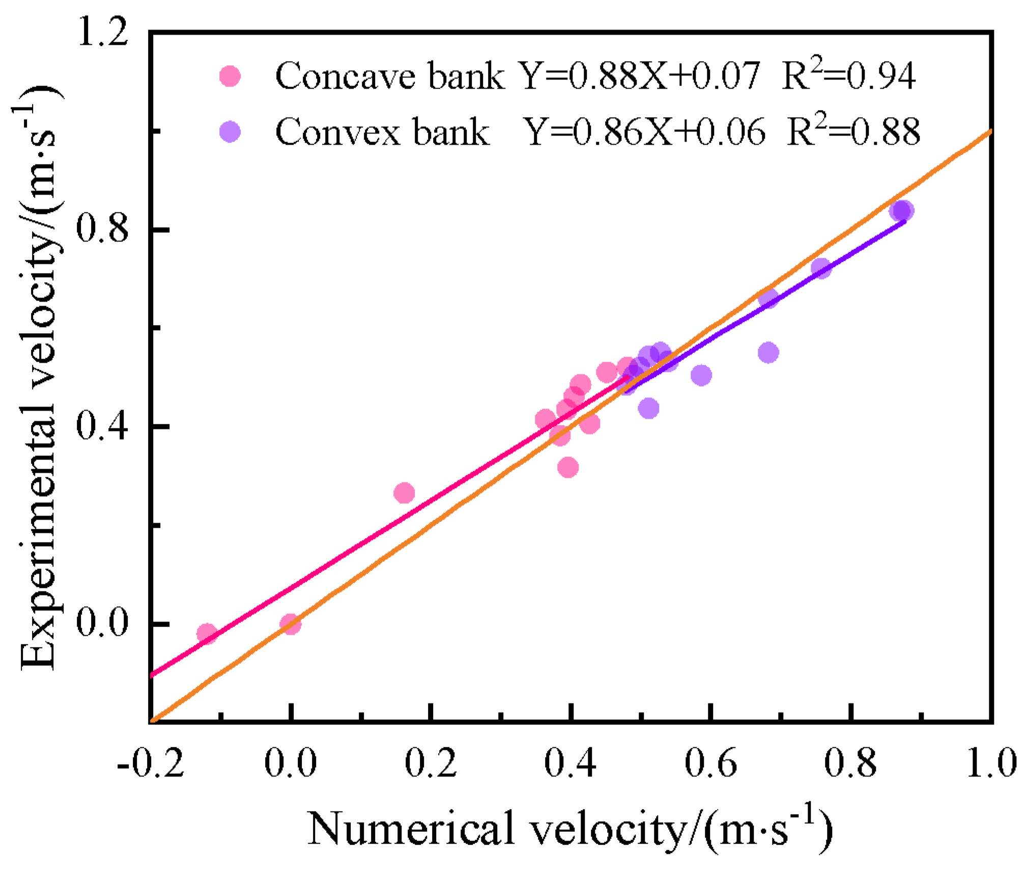
2.4. Numerical Model Validation

In order to visually reflect the reliability of the numerical model, the correlation between the average experimental velocity and the average simulated velocity at a total of 24 measuring points at 50% water depth and 0.05 m from the concave and convex banks was determined (Figure 3).

The results of the correlation analysis show that the flow velocity is lower on the outer bank side, whereas it is larger on the inner bank side, which is caused by the forced change in the flow direction and the shrinkage of the cross section. The flow velocities at most measuring points range between 0.4 m/s and 0.6 m/s, which is consistent with experimentally obtained values. Comparison of the correlation coefficients of the concave and convex banks indicates that the correlation coefficient of the convex bank is lower, because the concave and convex banks show different degrees of turbulence in the flow process, and there are also errors in the physical experiment measurements. In general, the results of the physical experiments are in good agreement with the results of the numerical simulation; so, this numerical model can be used for subsequent numerical simulation studies. The results of the third section are all based on the validated turbulence model from the second section.

3. Results

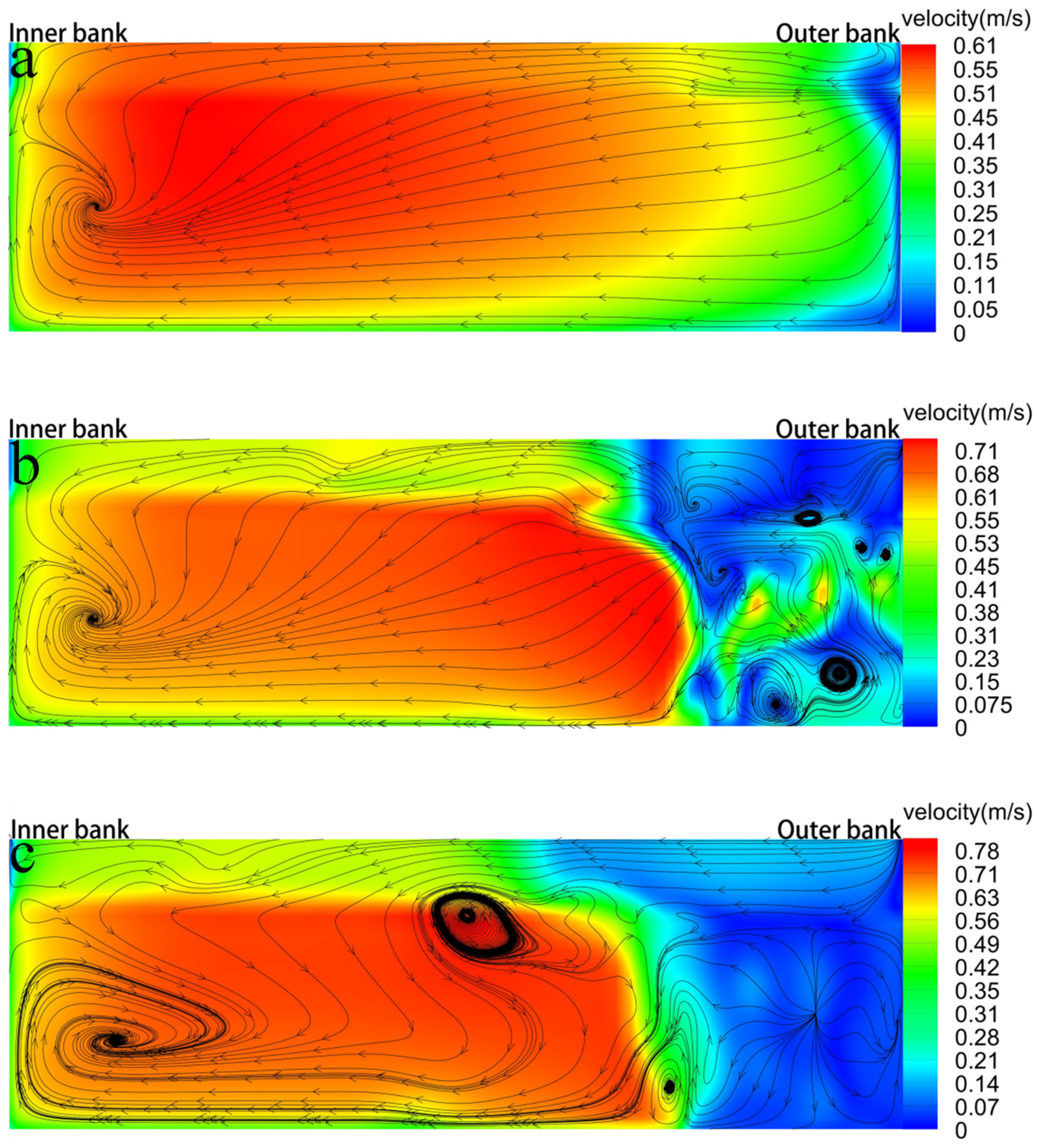
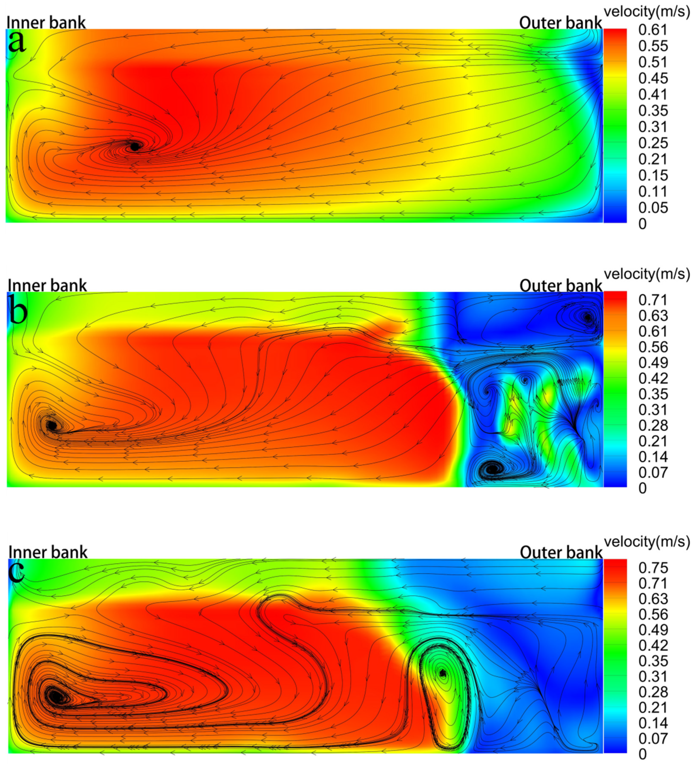
3.1. Mean Flow Pattern

The flow velocity and flow pattern in the channels with different degrees of curvature are described in this section. Figure 4 shows the time-averaged streamlines and time-averaged velocities in three sections that are perpendicular to the main flow direction in the 45° bend. Figure 5 and Figure 6 show the same data for the 90° and 180° bends, respectively.

Figure 4a, Figure 5a and Figure 6a indicate that the bending degree of the river does not significantly alter the flow pattern of the outer bank. The streamlines are arranged in an orderly fashion, and the streamlines point from the outer bank to the inner bank. Secondary flow is clearly visible at the inner bank. The SSF at Section a in the 45° bend is lower than that in the 90° bend, whereas the SSF at Section a in the 180° bend is significantly higher than that in the other two bends. Two vortices are observed in the 180° bend with the highest SSF, indicating that the flow is more intense in the radial and vertical directions. There is a significant difference in the flow velocity between the two sides of the river, with flow velocity at the outer bank being lower than that at the inner bank. This is due to the fact that the flow is constrained by the permeable spur dike. The placement of the permeable spur dike on the outer bank side causes a drastic change in the flow direction and a sudden decrease in the cross section, resulting in a higher flow velocity on the inner bank side.

The sections in Figure 4b, Figure 5b and Figure 6b are located within the permeable spur dike. Weak secondary flow appears at the outer bank, and multiple small eddies are generated. The flow passes through the permeable hole, which increases the flow velocity near the permeable hole and reduces the radial flow velocity within the spur dike. The vortices mainly appear near the permeable holes, because the permeable holes interfere with the flow pattern within the spur dike. The obstruction produced by the obstacle should generate a well-developed vortex, but because the water flow carries energy to escape from the permeable holes, the vortex energy is continuously dissipated. Therefore, the vortex is generated at the outer bank (Figure 4b, Figure 5b and Figure 6b), but it is not fully developed. The velocity at the inner bank is higher than that at the outer bank, and there is a secondary flow. At this time, the blocking effect of the permeable spur dike on the tangential velocity is enhanced, which leads to an obvious difference between the velocities at the outer and inner banks, and the tangential time-averaged velocity of the outer bank decreases, which reduces the scouring of the outer bank. The higher velocity at the outer bank is distributed near the permeable hole, which helps maintain the structural stability of the permeable spur dike. The increase in velocity at the inner bank helps reduce sediment deposition. On the side of the bank on which the spur dike is not placed, the secondary flow produces a clockwise vortex at the bank opposite the spur dike, and this vortex helps prevents the deposition of sediment at the inner bank and the migration of the river channel in the direction of the outer bank.

Figure 4c, Figure 5c and Figure 6c reveal that the blocking effect of the permeable spur dike on the water flow begins to weaken at this time, and a vortex appears near the dam head, which gradually moves to the upper left as the bending degree of the river decreases. At the cross section in Figure 4c, the outer bank generates a streamline that is radial. At the cross section in Figure 5c, the outer bank generates a streamline moving upward, and at the cross section in Figure 6c, the outer bank generates a secondary flow, forming a vortex. Figure 4c, Figure 5c and Figure 6c indicate that the secondary flow is formed at the inner bank, and the vortex generated by the secondary flow is close to the inner bank, forming an upward streamline at the inner bank to further prevent sediment deposition at the inside bank.

Figure 7, Figure 8 and Figure 9 show the time-averaged flow velocity and time-average streamlines on the plane at water depths of 10% (a) and 90% (b) in the 45°, 90°, and 180° bends, respectively. In the bend channel, the flow pattern is relatively complex. By observing the profile perpendicular to the water depth direction, we can understand the changes in the flow pattern near the permeable spur dike.

The general direction of the water flow is determined by the combined action of the centrifugal force in the curved channel and the spur dike. Figure 7, Figure 8 and Figure 9 indicate that when the water flow passes through them, the permeable spur dikes constrain the water flow and force it to flow toward the inner bank. The flow direction is mainly determined by the spur dike. After passing through the spur dike, the restraint on the water flow no longer exists, and the water flow begins to flow to the outer bank. By comparing the streamlines and velocities at different depths in any curved channel, we find that the streamlines near the riverbed are quite different from those far away from the riverbed, and the streamlines near the riverbed exhibit an obvious trend of moving to the outer bank. A comparison of the time-averaged streamlines and velocities in Sections a and b in the same bend reveals that at Section a, near the riverbed, the streamlines begin to move to the outer bank after passing through the spur dike, and a backflow region is formed, and the center of the vortex appears at the position 5.5 times L behind the permeable spur dikes. Moreover, at a position far away from the riverbed from Section b, the backflow area also appears behind the permeable spur dikes, and the vortex center appears at the position 6.5 times L behind the permeable spur dikes, but the streamline does not move significantly toward the outer bank at this time. In Section a, near the riverbed in the 45° bend, an anticlockwise vortex appears near the head of the spur dike, and a flow opposite to the mainstream appears near the outer bank. At the same position in the 90° bend, the streamlines appear inside the permeable spur dike and point downstream. In the 180° bend, a complex vortex system is seen in the permeable spur dike, which indicates that the SSF is high here. In the 45° bend, radial flow is observed in Section b far away from the riverbed, and the flow between the horseshoe vortex and the radial flow is observed in the area 1.5 times L behind the spur dike. In the 90° bend, radial flow occurs in the permeable spur dike, and the flow behind the permeable spur dike points upstream. In the 180° bend, the flow in the permeable spur dike points upstream, and the counterclockwise vortex appears behind the spur dike near the dam head. There is no large-scale vortex in the permeable spur dike, because part of the kinetic energy carried by the flow is conveyed through the permeable hole, and the kinetic energy within the permeable spur dike cannot maintain the development of the vortex. Thus, only a low-flow-velocity area is formed in the permeable spur dike, which helps reduce the internal scouring of the permeable spur dike by the flow and is both conducive to the structural stability of the spur dike and effectively protective of the outer bank. In general, in Sections a and b in Figure 7, Figure 8 and Figure 9, the time-averaged streamlines near the inner bank are arranged in order, and the time-averaged velocity is large. Near the outer bank, a large low-velocity area is formed behind the permeable spur dike, accompanied by backflow, which favors sediment deposition, repairing the damaged river channel and improving the stability of the outer bank.

Figure 10 represents the contour plots of the dimensionless mean velocity field in the 50% water depth plane in the 45°, 90°, and 180° bends. The region of higher tangential flow velocity is found to be located downstream. The high-flow-velocity region is concentrated along the inner bank as a result of the forced change in the main flow direction caused by the spur dike, which causes the main flow to be preferentially located along the inner bank. The low-flow-velocity region is concentrated downstream of the spur dike within a distance seven to nine times the length of the spur dike, and the width of the low-flow-velocity region is smaller than the length of the spur dike. The abrupt change in flow velocity in the excess area indicates the formation of a strong shear layer. The high-flow-velocity area between the inner bank and spur dike shows a jagged contour. This jagged contour is more pronounced in the 180° bend due to periodic fluctuations in the velocity gradient along the radial direction, suggesting that a high-intensity shear layer is generated in the high-curvature bend. The increased curvature of the bend and the gradual migration of the high-flow-velocity region toward the inner bank implies that the inner bank is at risk of erosion, which contrasts with the traditional concept of bank protection. The flow velocity in the low-flow-velocity region downstream of the outer bank’s permeable spur dike is only 0.1–0.5 times the average flow velocity, indicating that the permeable spur dike protects the outer bank. The radial flow velocity contour map reveals that the excessive radial flow velocity area envelopes the head of the spur dike, and high radial flow velocity occurs locally at the head of the spur dike. Negative flow velocity (radial flow velocity is negative from the inner bank to the outer bank) is mainly distributed in the downstream area, the flow velocity is low (0.05–0.1 times the average flow velocity), and the area of negative flow velocity area in the 180° bend exhibits a gradual increase. The maximum radial flow velocity accounts for 20% of the mean flow velocity, indicating that secondary flow is generated in the bend. The vertical flow velocity contour plots reveal that the vertical flow velocity at the head of the spur dike shows negative values (vertical flow velocity is negative from top to bottom), indicating that the water surface line is lower here, which is consistent with laboratory observations. A band of negative-flow-velocity zones appears downstream from the head of the spur dike, showing a distinct band in the 180° bend. In the 90° bend, this band more closely resembles the annular flow velocity distribution produced by a cylindrical bypass.

3.2. Strength of Secondary Flow

The presence of a permeable spur dike in a meandering channel induces a change in the flow pattern. This section focuses on the change in the strength of secondary flow (SSF). The SSF is an important factor affecting the stability of meandering channels. In this study, the SSF was calculated according to the method described by Shukry [48]. This method uses the lateral kinetic energy of each section in the channel divided by the total kinetic energy to obtain the SSF.

$$SSF=\frac{K_{latral}}{K_{total}}=\frac{{\left(\overline{v_r}\right)}^2+{\left(\overline{w_v}\right)}^2}{{\left(\overline{u_t}\right)}^2+{\left(\overline{v_r}\right)}^2+{\left(\overline{w_v}\right)}^2}$$

(8)

The overline in the formula indicates the time-averaged value. In the formula, $K_{latral}$ is the transverse kinetic energy, $K_{total}$ is the total kinetic energy of any section, and $\overline{u_t}$, $\overline{v_r}$, and $\overline{w_v}$ are the tangential, radial, and vertical time-averaged velocities, respectively.

Figure 11 clearly shows that there is no drastic change in the SSF between 1.4 m and 2.5 m (9.3 to 16.7 times L) from the inlet of the bend upstream of the permeable spur dike, but it is worth noting that the SSF increases significantly as the bend curvature increases. When the bend curvature increases from 0.125 (45° bend) to 0.25 (90° bend), the SSF increases by 3.6 times, and when the bend curvature increases from 0.25 (90° bend) to 0.5 (180° bend), the SSF increases by 3 times. This is because upstream of the permeable spur dike, within a distance of 2.5 m from the bend entrance, the permeable spur dike has little influence on the flow pattern, and the transverse kinetic energy of the flow is generally low in the three channels with different curvatures. At this time, the transverse kinetic energy of the bend with a curvature of 0.5 is larger than that of the other types of bends. In the range of 2.5 m to 2.8 m (16.7 to 18.7 times L) from the entrance of the bend, the SSF increases sharply, which is due to the fact that the spur dikes strengthen the binding effect on the flow and the cross section begins to reduce in size, resulting in a rapid increase in the lateral kinetic energy. Although the total kinetic energy is also increasing, the lateral kinetic energy is dominant. Within the bend, the SSF begins to fluctuate significantly and assumes a reduced attitude within the range of 2.8 m to 4.5 m (between 18.7 and 30 times L). In this region, it is obvious that the flow pattern is disturbed by the spur dike. This disturbance occurs at a distance of 3.14 m (20.9 times L) from the bend inlet, whereas the peak SSF occurs at a distance of 3.22 m (21.5 times L) from the bend inlet, which is located in the spur dike field and adjacent to the second spur dike. Figure 11 reveals that the position of the peak value of the SSF is almost the same after the spur dike is placed in the three channels with different curvatures, and when the curvature of the bend is 0.5, the peak value of the SSF is significantly higher than that of the bends with curvatures of 0.25 and 0.125. This is because the bend curvature is too large in the latter two cases, and the binding effect on the flow is strengthened due to the increase in the radial and vertical kinetic energy of the flow. At 3.22 m from the bend entrance, the SSF reaches its peak value and begins to decline, which is due to the increase in the area of the cross section and the gradual decrease in the total kinetic energy of any section in this area. Owing to the interference of the backflow behind the spur dike, the lateral kinetic energy fluctuates continuously and exhibits a downward trend as a whole. From 4.5 m away from the entrance of the bend, the flow pattern gradually begins to recover, and the fluctuation of the SSF almost disappears and slowly declines until it is stable.

3.3. Turbulent Kinetic Energy

Turbulent kinetic energy is used to describe the intensity of turbulence, and the greater the turbulent kinetic energy, the more violent the collision and separation within the fluid. In this study, the normalized turbulent kinetic energy (NTKE) was calculated according to the method proposed by Kumar and Ojha [49]. This method uses the mean value of the square of the tangential, radial, and vertical fluctuating velocities in each section of the channel and divides it by the average shear velocity to obtain the NTKE.

$$NTKE=\frac{1}{u_{\ast }{}^2}\left(\overline{u_t^{\prime }{}^2}+\overline{v_r^{\prime }{}^2}+\overline{w_v^{\prime }{}^2}\right),$$

(9)

The overline in the formula indicates the time-averaged value. $u_t^{\prime }$, $v_r^{\prime }$, and $w_v^{\prime }$ are the tangential, radial, and vertical fluctuating velocities, respectively. $u_{\ast }=\sqrt{Rgs}$ is the average shear velocity of the flow at the entrance of the open channel. $g$ is the acceleration of gravity. $R$ is the hydraulic radius. $s$ is the slope of the open channel.

Figure 12 shows the NTKE in 45 radial sections. This figure shows that the NTKE values of open channels with three different curvatures change synchronously within 3 m from the entrance of the bend (20 times L), and the NTKE intensities are low. Subsequently, the NTKE begins to increase, and the peak value of the NTKE intensity appears 3.14 m away from the bend entrance, which corresponds to the location of the spur dike. The permeable spur dike in the open channel reduced the area of the cross section and caused the velocity to increase sharply, which in turn enhanced the fluctuating velocity and the internal collision and separation of the fluid. This is the reason for the sharp increase in NTKE. It is worth noting that the peak value of the NTKE intensity in the bend with the curvature of 0.125 was the largest and was followed by that of the bend with a curvature of 0.5. The fluid collision and separation motion were very violent near the permeable spur dike, and the fluctuation intensity at this position was the most prominent in the whole open channel. The fluctuation intensity near the permeable spur dike in the bend with a curvature of 0.125 was the greatest, followed in decreasing order of magnitude by the fluctuation intensities near the permeable spur dikes in the bends with curvatures of 0.5 and 0.25. The NTKE intensity of the three curved channels with different curvatures began to decrease synchronously and fluctuate in different degrees between the two sections with distances of 3.14 m and 4.19 m from the entrance of the curved channel. This is because, as the flow passes through the permeable spur dike and gradually moves away from it, the internal collision and separation movement of the fluid begins to weaken, and the flow begins to recover towards the open-channel flow. Between the two profiles, the NTKE intensity in the bend with the curvature of 0.5 fluctuated slightly, and the NTKE intensity began to increase slightly near the entrance of the bend at a distance of 3.31 m, although it was generally lower than that in the bends with curvatures of 0.125 and 0.25. This is because the pulsation intensity downstream of the permeable spur dike was generally low within the bend with a curvature of 0.5. It is worth noting that at distances between 3.25 m and 4.19 m from the entrance of the curve, the NTKE decreased as the bend curvature increased. Moreover, the NTKE decreased from 4.19 m from the entrance of the curve in all three curves. Figure 12 demonstrates that the NTKE in the bend with a curvature of 0.125 began to decrease first, followed by the NTKE in the bends with curvatures of 0.25 and 0.5. This indicates that the fluctuating velocity in the bend with a curvature of 0.125 began to decrease first, followed by the fluctuating velocity in the bend with a curvature of 0.25. The fluctuating velocity in the bend with the curvature of 0.5 also began to decrease after a small increase.

4. Discussion

The permeable spur dike effectively reduces the flow velocity along the outer bank and forces the main flow to move towards the inner bank. Thus, a clockwise-spiraling downstream flow line is formed near the inner bank. The center of the flow line is located near the 50% water depth, and the spiraling flow line is located in the high-flow-velocity zone, suggesting the occurrence of secondary flow, which may cause the scouring of the inner bank. Therefore, it is necessary to evaluate the stability of the inner bank when constructing spur dikes in relatively narrow bends. The flow velocity between two permeable spur dikes is high near the permeable holes, and the counterclockwise vortex is enveloped by the low-flow-velocity zone. The vortex forms near the streambed along the outer bank, which could threaten the stability of the spur dikes. Therefore, it is necessary to reinforce the connection between the spur dikes and the streambed when constructing the river training building. In this study, the velocity distribution in different bends was compared in a high-Reynolds-number flow, and it was found that the tangential velocity near the inner bank in a 180° bend showed a jagged distribution, which was due to periodic fluctuations in the velocity gradient along the radial direction, generating a high-intensity shear layer. This phenomenon was not pronounced in low-curvature bends and was more prominent in high-Reynolds-number flows, as shown by the flume test of Jeon et al. [50]. The shortcoming of this study is that there was no comparison between high- and low-Reynolds-number flows.

While the construction of spur dikes can change the SSF in a river channel, the curvature of the bend also has a critical impact on changes in the SSF. The results of this study show that the SSF in the bend increases as the bend curvature increases, and the SSF is maximum at the cross-sectional location where the spur dike is located, which implies that the protective effect of the spur dike on the outer bank and the riverbed decreases as the bend curvature increases. However, only three bends were evaluated in this study, and therefore, a detailed analysis of the relationship between bend curvature and the SSF could not be conducted. Furthermore, the erosion effect could not be evaluated; so, the effect of spur dikes on the riverbed and the outer bank should be evaluated in the future management of high-curvature channels so as to determine whether to increase the length of the spur dike to increase the extent of the low-flow zone. The trends in the SSF observed by Vaghefi et al. [51] were similar to those observed in the current study, but they only studied a 90° bend, and the maximum value of the SSF was 1.7 times higher than that in the current study. This is because they used impervious spur dikes in their tests, which resulted in higher radial and vertical flow velocities than those observed in the current study. The present study differs from that of Vaghefi et al. [51] in that it compares the variation in the SSF along different bends, and in combination with their study, we found that changing the wing length ratio of the spur dike has a less pronounced effect on the secondary flow in the bend than changing the curvature of the bend.

The NTKE is not only affected by the bend curvature but also differs among the three bends at the same position from the bend inlet. The results show that the NTKE is not significantly affected by changes in bend curvature at distances of 0–3 m from the bend inlet. The NTKE peaks at the cross section where the spur dike is located, indicating that the spur dike is able to significantly increase the NTKE in the bend, which will increase the head loss and exert a positive effect on downstream riverbed stability. The NTKE at distances of 3.14–4.19 m from the entrance of the bend is closely related to the curvature of the bend; when the curvature of the bend increases, the NTKE decreases, suggesting that the head loss in the high-curvature bend is smaller at distances of 3.14–4.19 m, which implies that as the curvature of the bend increases, the energy dissipation effect brought about by the spur dike diminishes. Therefore, when evaluating the energy dissipation efficacy of spur dikes, the present study considers it necessary to evaluate the curvature of the bend along with the energy dissipation effect of the spur dike. Ding et al. [52] studied spur dikes of different lengths, finding that the NTKE peaks at the head of the spur dike and that the NTKE for the outer bank is greater than that for the inner bank at the cross section at which the spur dike is situated, due to the collision of the spur dike with the flow, which forces a change in the direction of the flow and increases outer bank collision and separation within the fluid. These findings are similar to the findings of the present study. The present study differs from that of Ding et al. [52] in that it compares the variation in NTKE along the course of the three bends. The limitation of this study is that it did not include a comparative evaluation of spur dikes with different lengths and different pick angles. The shape of the spur dike used in this study is a regular rectangle, and irregularly shaped obstacles can bring about a higher head loss; so, it is necessary to investigate the energy dissipation effect of spur dikes with different shapes. RANS simulations struggle to capture small-scale structures in turbulent flow. They rely on turbulence models, and different turbulence models may have varying applicability to different flow conditions. RANS simulations are highly dependent on the mesh, and the quality of the mesh can affect the accuracy of the simulation. Therefore, it is important to be mindful of this when using RANS models.

5. Conclusions

In this study, the RNG k-ε turbulence model was used to analyze the effects of permeable spur dikes on mean flow pattern, SSF, and NTKE in different bends. The conclusions of the study are as follows:

(1) The correlation coefficients between the numerically simulated and experimental flow velocities near the concave and convex banks of the 180° bend are 0.94 and 0.88, while the correlation coefficients for the convex bank are lower, because the water near the concave and convex banks exhibits different degrees of turbulence in the flow process, and because there are errors in the physical experimental measurements. The numerical simulation correlation is required to be greater than 0.8 in engineering applications; so, the results of this numerical simulation are reliable.

(2) The SSF upstream of the permeable spur dike in the 45° bend is low, whereas that in the 90° bend is obviously enhanced. Two vortices are observed in the 180° bend, which has the highest SSF, indicating that the flow is more intense in the radial and vertical directions in the 180° bend. There is a clear difference between the velocities at the outer and inner banks. The velocity at the outer bank is low, whereas that at the inner bank is large, and the overall velocity decreases as the bending degree of the river increases. The permeable holes in the spur dike allow a part of the flow to pass through, which reduces the radial and vertical flow within the permeable spur dike. The presence of obstacles should result in the formation of an obvious vortex, but the energy of the vortex is continuously dissipated as the energy carried by the flow escapes through the permeable holes. The blocking effect of the permeable spur dike on the longitudinal velocity is enhanced, which leads to an obvious difference between the velocities at the outer and inner banks. Moreover, the tangential time-averaged velocity at the outer bank decreases, which reduces the scouring of the outer bank. The higher velocity at the outer bank is distributed near the permeable hole, which helps to maintain the structural stability of the permeable spur dike. The increase in velocity at the inner bank helps reduce sediment deposition. Near the inner bank, the secondary flow produces a clockwise vortex, which helps prevent sediment deposition at the inner bank and also helps prevent the migration of the channel in the direction of the outer bank. The time-averaged streamlines near the inner bank are arranged in order, and the time-averaged velocity is relatively high. Near the outer bank, a large low-velocity area is formed behind the permeable spur dike, accompanied by backflow. This is conducive to sediment deposition, which helps repair the damaged river channel and improves the stability of the outer bank.

(3) Upstream of the permeable spur dike, the SSF increases obviously as the bend curvature increases. However, in the vicinity of the permeable spur dike and within the range of eight times L downstream, the SSF does not change significantly as the bend curvature changes. The peak of the SSF occurs at a distance of 3.22 m (21.5 times L) from the inlet of the bend, which is located in the spur dike field and close to the second spur dike. For the three channels with different curvatures, the positions of the peak values of the SSF are almost identical after the permeable spur dikes are placed. Considering the three bends with different curvatures, the SSF changes gently upstream of the permeable spur dike, reaching the peak value at the point where the permeable spur dikes are positioned, after which the fluctuation begins to reduce and gradually stabilize.

(4) Within the range of 3 m from the entrance of the bend, the NTKE values of the three open channels with different curvatures change synchronously, and the intensity of the NTKE is small. The peak value of NTKE intensity appears 3.14 m away from the entrance of the bend, which corresponds to the location of the permeable spur dike. The peak value of NTKE intensity is the highest, and the fluctuating intensity near the permeable spur dike is the most intense in the bend with the curvature of 0.125, followed by that in the bend with the curvature of 0.5. The fluctuation intensity is the lowest and shows a decreasing trend, and the NTKE intensity is the lowest in the bend with the curvature of 0.25. Within the range of 6.5 times L downstream (3.25 m to 4.19 m from the entrance of the bend), the NTKE decreases as the bend curvature increases. For the three channels with different curvatures, the NTKE changes smoothly upstream of the permeable spur dike, reaching a maximum near the permeable spur dike, after which the fluctuations begin to decline and the NTKE gradually stabilizes.

References

1. Bernhardt, E.S.; Palmer, M.A.; Allan, J.D.; Alexander, G.; Barnas, K.; Brooks, S.; Carr, J.; Clayton, S.; Dahm, C.; Follstad-Shah, J. Synthesizing U.S. River Restoration Efforts. Science 2005, 308, 636–637. [Google Scholar] [CrossRef] [PubMed]
2. Iqbal, S.; Pasha, G.A.; Ghani, U.; Ullah, M.K.; Ahmed, A. Flow Dynamics Around Permeable Spur Dike in a Rectangular Channel. Arab. J. Sci. Eng. 2021, 46, 4999–5011. [Google Scholar] [CrossRef]
3. Gu, Z.P.; Akahori, R.; Ikeda, S. Study on the Transport of Suspended Sediment in an Open Channel Flow with Permeable Spur Dikes. Int. J. Sediment. Res. 2011, 26, 96–111. [Google Scholar] [CrossRef]
4. Ettema, R.; Kirkil, G.; Muste, M. Similitude of Large-Scale Turbulence in Experiments on Local Scour at Cylinders. J. Hydraul. Eng. 2006, 132, 33–40. [Google Scholar] [CrossRef]
5. Kuhnle, R.A.; Alonso, C.V.; Shields, F.D. Geometry of Scour Holes Associated with 90 Spur Dikes. J. Hydraul. Eng. 1999, 125, 972–978. [Google Scholar] [CrossRef]
6. Hu, J.; Wang, G.; Wang, P.; Yu, T.; Chen, H. Experimental Study on the Influence of New Permeable Spur Dikes on Local Scour of Navigation Channel. Sustainability 2022, 15, 570. [Google Scholar] [CrossRef]
7. Nayyer, S.; Farzin, S.; Karami, H.; Rostami, M. A Numerical and Experimental Investigation of the Effects of Combination of Spur Dikes in Series on a Flow Field. J. Braz. Soc. Mech. Sci. 2019, 41, 256. [Google Scholar] [CrossRef]
8. Rajaratnam, N.; Nwachukwu, B. Erosion near Groyne-Like Structures. J. Hydraul. Res. 1983, 21, 277–287. [Google Scholar] [CrossRef]
9. Przedwojski, B. Bed Topography and Local Scour in Rivers with Banks Protected by Groynes. J. Hydraul. Res. 1995, 33, 257–273. [Google Scholar] [CrossRef]
10. Ettema, R.; Muste, M. Scale Effects in Flume Experiments on Flow around a Spur Dike in Flatbed Channel. J. Hydraul. Eng. 2004, 130, 635–646. [Google Scholar] [CrossRef]
11. Fazli, M.; Ghodsian, M.; Neyshabouri, S.A. Scour and Flow Field around a Spur Dike in a 90° bend. Int. J. Sediment. Res. 2008, 23, 56–68. [Google Scholar] [CrossRef]
12. Kothyari, U.C.; Raju, K.G.R. Scour around Spur Dikes and Bridge Abutments. J. Uydraul. Res. 2001, 39, 367–374. [Google Scholar] [CrossRef]
13. Kuhnle, R.A.; Alonso, C.V.; Shields, F.D. Local Scour Associated with Angled Spur Dikes. J. Hydraul. Eng. 2002, 128, 1087–1093. [Google Scholar] [CrossRef]
14. Ikeda, S.; Sugimoto, T.; Yoshiike, T. Study on the Characteristics of Flow in Channels with Impermeable Spur Dikes. Proc. JSCE 2000, 656, 145–155. [Google Scholar] [CrossRef] [PubMed]
15. Haghnazar, H.; Hashemzadeh Ansar, B.; Asadzadeh, F.; Salehi Neyshabouri, A.A. Experimental Study on the Effect of Single Spur Dike with Slope Sides on Local Scour Pattern. J. Civ. Eng. Mater. Appl. 2018, 2, 111–120. [Google Scholar]
16. Azamathulla, H.M.; Ab Ghani, A.; Zakaria, N.A.; Guven, A. Genetic Programming to Predict Bridge Pier Scour. J. Hydraul. Eng. 2010, 136, 165–169. [Google Scholar] [CrossRef]
17. Azamathulla, H.M.; Yusoff, M.A.M. Soft Computing for Prediction of River Pipeline Scour Depth. Neural. Comput. Appl. 2013, 23, 2465–2469. [Google Scholar] [CrossRef]
18. Pandey, M.; Lam, W.H.; Cui, Y.G.; Khan, M.A.; Singh, U.K.; Ahmad, Z. Scour around Spur Dike in Sand–Gravel Mixture Bed. Water 2019, 11, 1417. [Google Scholar] [CrossRef]
19. Masjedi, A.; Bejestan, M.S.; Moradi, A. Experimental Study on the Time Development of Local Scour at a Spur Dike in a 180° Flume Bend. J. Food Agric. Environ. 2010, 8, 904–907. [Google Scholar]
20. Fukuoka, S.; Watanabe, A.; Kawaguchi, H.; Yasutake, Y. A Study of Permeable Groins in Series Installed in a Straight Channel. Proc. Hydraul. Eng. 2000, 44, 1047–1052. [Google Scholar] [CrossRef]
21. Li, Z.; Michioku, K.; Maeno, S.; Ushita, T.; Fujii, A. Hydraulic Characteristics of a Group of Permeable Groins Constructed in an Open Channel Flow. J. Appl. Mech. 2005, 8, 773–782. [Google Scholar] [CrossRef]
22. Osman, M.A.; Saeed, H.N. Local Scour Depth at the Nose of Permeable and Impermeable Spur Dikes. Univ. Khartoum Eng. J. 2012, 2, 1–9. [Google Scholar]
23. Zhou, Y.J.; Qian, S.; Sun, N.N. Application of Permeable Spur Dike in Mountain River Training. In Applied Mechanics and Materials; Trans Tech Publications Ltd.: Stafa, Switzerland, 2014; pp. 236–240. [Google Scholar]
24. Elawady, E.; Michiue, M.; Hinokidani, O. Movable Bed Scour around Submerged Spur Dikes. Proc. Hydraul. Eng. 2001, 45, 373–378. [Google Scholar] [CrossRef]
25. Nath, D.; Misra, U.K. Experimental Study of Local Scour around Single Spur Dike in an open Channel. Int. Res. J. Eng. Technol. 2017, 4, 2728–2734. [Google Scholar]
26. Li, Y.; Altinakar, M. Effects of a Permeable Hydraulic Flashboard Spur Dike on Scour and Deposition Yujian. In World Environmental and Water Resources Congress; ASCE: New York, NY, USA, 2016; pp. 399–409. [Google Scholar]
27. El-Raheem, A.; Ali, N.A.; Tominaga, A.; Khodary, S.M. Flow analysis around groyne with different permeability in compound channel flood plains. J. Eng. Sci. 2013, 41, 302–320. [Google Scholar]
28. Yun, B.; Yu, T.; Wang, P. Experiment research on energy variation around the permeable spur dike. Sci. Technol. Eng. 2021, 21, 3783–3789. [Google Scholar]
29. Fan, X.; He, W.; Zhao, W.; Yan, C. Study on variation law of flow structure of hydraulic flashboard permeable spur dike along with water permeability. Water Resour. Hydropower Eng. 2018, 49, 120–126. [Google Scholar]
30. Moreto, J.R.; Reeder, W.J.; Budwig, R.; Tonina, D.; Liu, X.F. Experimentally Mapping Water Surface Elevation, Velocity, and Pressure Fields of an Open Channel Flow Around a Stalk. Geophys. Res. Lett. 2022, 49, e2021GL096835. [Google Scholar] [CrossRef]
31. Westerweel, J.; Elsinga, G.E.; Adrian, R.J. Particle Image Velocimetry for Complex and Turbulent Flows. Annu. Rev. Fluid Mech. 2013, 45, 409–436. [Google Scholar] [CrossRef]
32. You, H.; Tinoco, R.O. Turbulent Coherent Flow Structures to Predict the Behavior of Particles with Low to Intermediate Stokes Number Between Submerged Obstacles in Streams. Water. Resour. Res. 2023, 59, e2022WR032439. [Google Scholar] [CrossRef]
33. He, C.; Taylor, J.N.; Rochfort, Q.; Nguyen, D. A New Portable in Situ Flume for Measuring Critical Shear Stress on River Beds. Int. J. Sediment. Res. 2021, 36, 235–242. [Google Scholar] [CrossRef]
34. Koken, M. Coherent Structures around Isolated Spur Dikes at Various Approach Flow Angles. J. Hydraul. Res. 2011, 49, 736–743. [Google Scholar] [CrossRef]
35. Koken, M.; Constantinescu, G. An Investigation of the Flow and Scour Mechanisms around Isolated Spur Dikes in a Shallow Open Channel: 1. Conditions corresponding to the initiation of the erosion and deposition process. Water. Resour. Res. 2008, 44, W08406. [Google Scholar] [CrossRef]
36. Koken, M.; Constantinescu, G. Flow and Turbulence Structure around a Spur Dike in a Channel with a Large Scour Hole. Water Resour. Res. 2011, 47, W12511. [Google Scholar] [CrossRef]
37. Koken, M.; Constantinescu, G. An Investigation of the Dynamics of Coherent Structures in a Turbulent Channel Flow with a Vertical Sidewall Obstruction. Phys. Fluids 2009, 21, 085104. [Google Scholar] [CrossRef]
38. Paik, J.; Escauriaza, C.; Sotiropoulos, F. Coherent Structure Dynamics in Turbulent Flows Past in-Stream Structures: Some Insights Gained Via Numerical Simulation. J. Hydraul. Eng. 2010, 136, 981–993. [Google Scholar] [CrossRef]
39. Paik, J.; Sotiropoulos, F. Coherent Structure Dynamics Upstream of a Long Rectangular Block at the Side of a Large Aspect Ratio Channel. Phys. Fluids 2005, 17, 115104. [Google Scholar] [CrossRef]
40. McCoy, A.; Constantinescu, G.; Weber, L. Exchange Processes in a Channel with Two Vertical Emerged Obstructions. Flow. Turbul. Combust. 2006, 77, 97–126. [Google Scholar] [CrossRef]
41. McCoy, A.; Constantinescu, G.; Weber, L. A Numerical Investigation of Coherent Structures and Mass Exchange Processes in Channel Flow with Two Lateral Submerged Groynes. Water. Resour. Res. 2007, 43, W05445. [Google Scholar] [CrossRef]
42. McCoy, A.; Constantinescu, G.; Weber, L.J. Numerical Investigation of Flow Hydrodynamics in a Channel with a Series of Groynes. J. Hydraul. Eng. 2008, 134, 157–172. [Google Scholar] [CrossRef]
43. Zhang, H.; Nakagawa, H.; Kawaike, K.; Yasuyuki, B. Experiment and Simulation of Turbulent Flow in Local Scour around a Spur Dike. Int. J. Sediment. Res. 2009, 24, 33–45. [Google Scholar] [CrossRef]
44. Haider, R.; Qiao, D.S.; Yan, J.; Ning, D.Z.; Pasha, G.A.; Iqbal, S. Flow Characteristics around Permeable Spur Dike with Different Staggered Pores at Varying Angles. Arab. J. Sci. Eng. 2022, 47, 5219–5236. [Google Scholar] [CrossRef]
45. Mulahasan, S.; Saleh, M.S.; Muhsun, S.S. Simulation of Flow around a Permeable Dike Using Physical and 3D-CFD Models. Int. J. River Basin Manag. 2021, 21, 53–65. [Google Scholar] [CrossRef]
46. Ouillon, S.; Dartus, D. Three-Dimensional Computation of Flow around Groyne. J. Hydraul. Eng. 1997, 123, 962–970. [Google Scholar] [CrossRef]
47. Yazdi, J.; Sarkardeh, H.; Azamathulla, H.M.; Ghani, A.A. 3D Simulation of Flow around a Single Spur Dike with Free-Surface Flow. Int. J. River Basin Manag. 2010, 8, 55–62. [Google Scholar] [CrossRef]
48. Shukry, A. Flow around Bends in an Open Flume. Trans. Am. Soc. Civ. Eng. 1950, 115, 751–778. [Google Scholar] [CrossRef]
49. Kumar, A.; Ojha, C.S.P. Effect of Different Compositions in Unsubmerged L-Head Groynes to Mean and Turbulent Flow Characteristics. KSCE J. Civ. Eng. 2019, 23, 4327–4338. [Google Scholar] [CrossRef]
50. Jeon, J.; Lee, J.Y.; Kang, S. Experimental Investigation of Three-Dimensional Flow Structure and Turbulent Flow Mechanisms around a Nonsubmerged Spur Dike with a Low Length-to-Depth Ratio. Water Resour. Res. 2018, 54, 3530–3556. [Google Scholar] [CrossRef]
51. Vaghefi, M.; Ahmadi, A.; Faraji, B. Variation of Hydraulic Parameters with Different Wing of a T-Shape Spur Dike in Bend Channels. J. Cent. South Univ. 2018, 25, 671–680. [Google Scholar] [CrossRef]
52. Ding, C.; Li, C.; Song, L.; Chen, S. Numerical Investigation on Flow Characteristics in a Mildly Meandering Channel with a Series of Groynes. Sustainability 2023, 15, 4124. [Google Scholar] [CrossRef]
Figure 1. Schematic diagram of numerical model calculation field.
Sustainability 15 15862 g001
Figure 2. Spur dike model parameters and layout.
Sustainability 15 15862 g002
Figure 3. Comparison of experimental and simulated values at 50% water depth, 5 cm from the concave and convex banks.
Sustainability 15 15862 g003
Figure 4. Time-averaged streamlines and time-averaged velocities over the cross sections at 20.5° (a), 22.5° (b), and 24.5° (c) in the 45° bend. The distances of sections (ac) from the entrance of the bend are 2.86 m, 3.14 m, and 3.42 m, respectively. The velocity cloud map is calculated as ( u ¯ ) 2 + ( v ¯ ) 2 + ( w ¯ ) 2 .
Sustainability 15 15862 g004
Figure 5. Time-averaged streamlines and time-averaged velocities over the cross sections at 41° (a), 45° (b), and 49° (c) in the 90° bend. The distances of sections (ac) from the entrance of the bend are 2.86 m, 3.14 m, and 3.42 m, respectively. The velocity cloud map is calculated as ( u ¯ ) 2 + ( v ¯ ) 2 + ( w ¯ ) 2 .
Sustainability 15 15862 g005
Figure 6. Time-averaged streamlines and time-averaged velocities over the cross sections at 82° (a), 90° (b), and 98° (c) in the 180° bend. The distances of sections (ac) from the entrance of the bend are 2.86 m, 3.14 m, and 3.42 m, respectively. The velocity cloud map is calculated as ( u ¯ ) 2 + ( v ¯ ) 2 + ( w ¯ ) 2 .
Sustainability 15 15862 g006
Figure 7. Time-averaged streamlines and time-averaged velocities over the cross section at (a) 10% and (b) 90% of the water depth in the 45° bend. The velocity cloud map is calculated as ( u ¯ ) 2 + ( v ¯ ) 2 + ( w ¯ ) 2 .
Sustainability 15 15862 g007
Figure 8. Time-averaged streamlines and time-averaged velocities over the cross section at (a) 10% and (b) 90% of the water depth in the 90° bend. The velocity cloud map is calculated as ( u ¯ ) 2 + ( v ¯ ) 2 + ( w ¯ ) 2 .
Sustainability 15 15862 g008
Figure 9. Time-averaged streamlines and time-averaged velocities over the cross section at (a) 10% and (b) 90% of the water depth in the 180° bend. The velocity cloud map is calculated as ( u ¯ ) 2 + ( v ¯ ) 2 + ( w ¯ ) 2 .
Sustainability 15 15862 g009
Figure 10. Contour plots of the dimensionless mean velocity field in the plane of 50% water depth in 45°, 90°, and 180° bends. Dimensionless tangential velocity: u ¯ / U 0 . Dimensionless radial velocity: w ¯ / U 0 . Dimensionless vertical velocity: v ¯ / U 0 .
Sustainability 15 15862 g010
Figure 11. Strength of secondary flow in the 45°, 90°, and 180° bends.
Sustainability 15 15862 g011
Figure 12. Normalized turbulent kinetic energy in the 45°, 90°, and 180° bends.
Sustainability 15 15862 g012