
Assessment of Climate Change’s Impact on Flow Quantity of the Mountainous Watershed of the Jajrood River in Iran Using Hydroclimatic Models


Abstract
:1. Introduction
- Identification of a climate model or a group of climate models from CMIP6, so as to create the highest correlation, using observations, in simulating the climate characteristics of the watershed [14].
- Regarding the set of new SSP scenarios in this study, these scenarios are assumptions that describe greenhouse gas emissions (GHGs) in the future. Compared to the scenarios of the representative concentration pathways (RCPs), climate changes are less considered in SSP scenarios; however, concerning greenhouse gases, they address higher CO2 emission levels. Based on the current condition of society, the new scenarios of CMIP6 describe socioeconomic drivers as the main factors. Shared socioeconomic pathway concentration projections (SSP1–2.6 to SSP5–8.5) show an acceptable trend of community growth in the 21st century [16].
2. Methodology
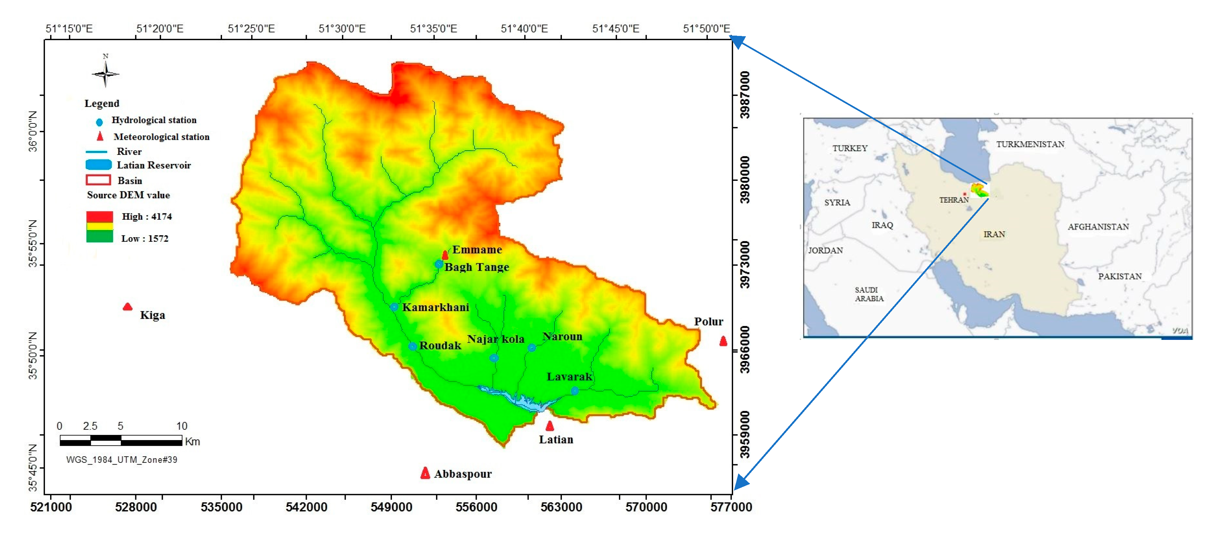
2.1. Case Study
2.2. SWAT
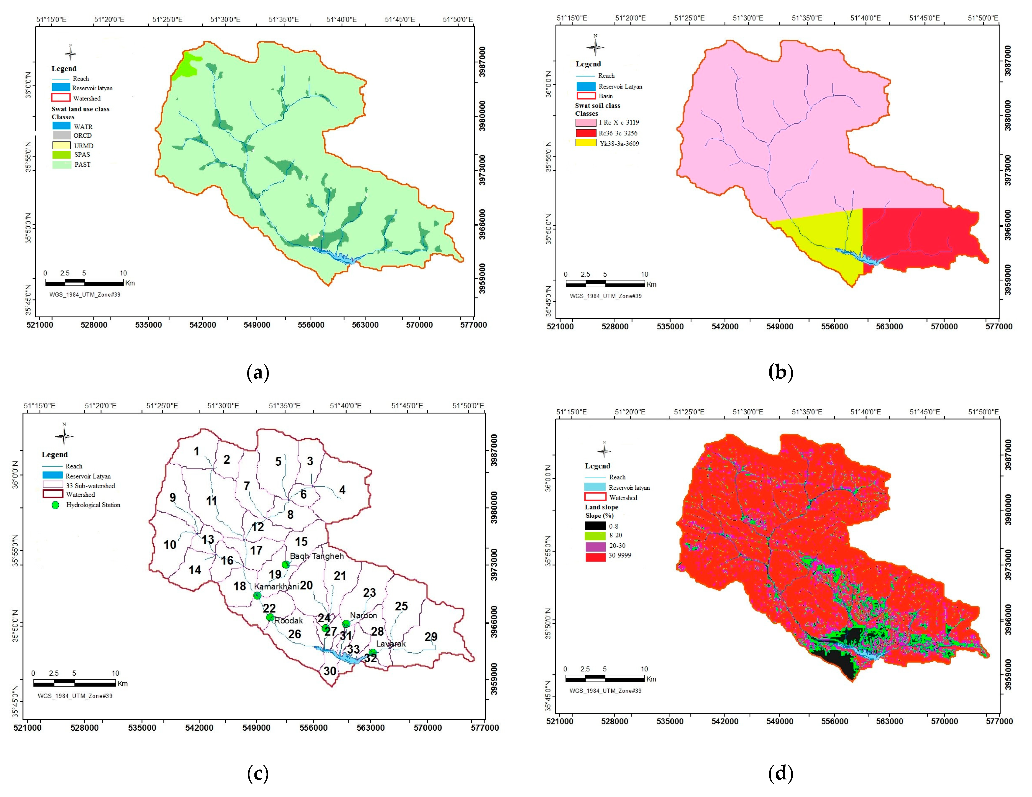
2.3. Input Data for Setting SWAT Model
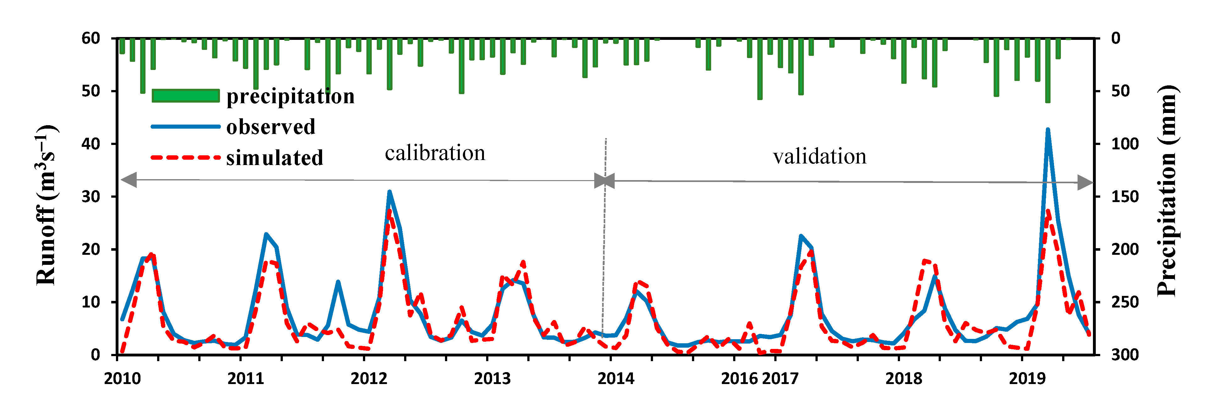
2.4. SWAT Calibration
2.5. Preprocessing of Climate Data
2.6. MRQNBC
3. Results
3.1. Hydrological Modeling
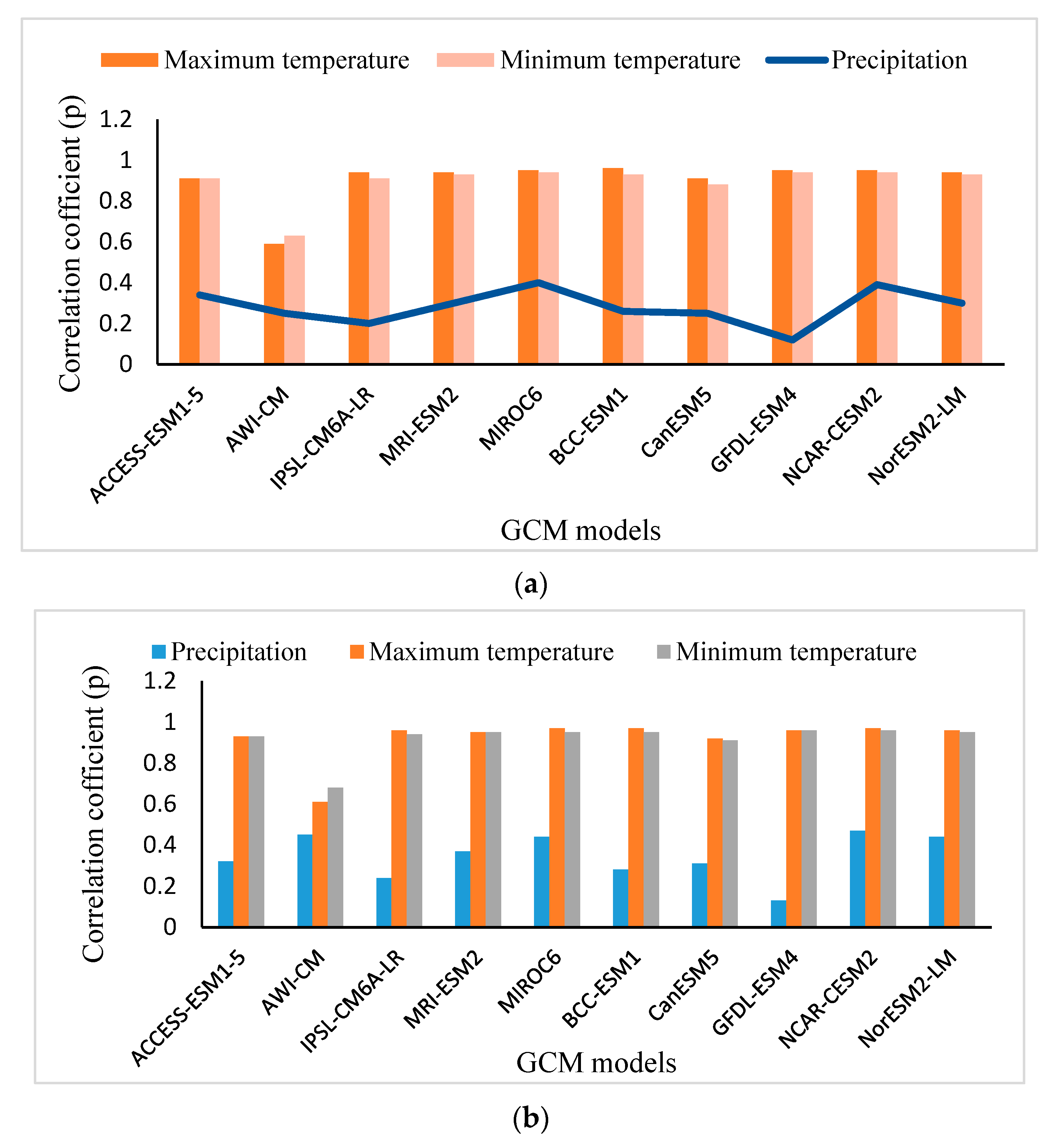
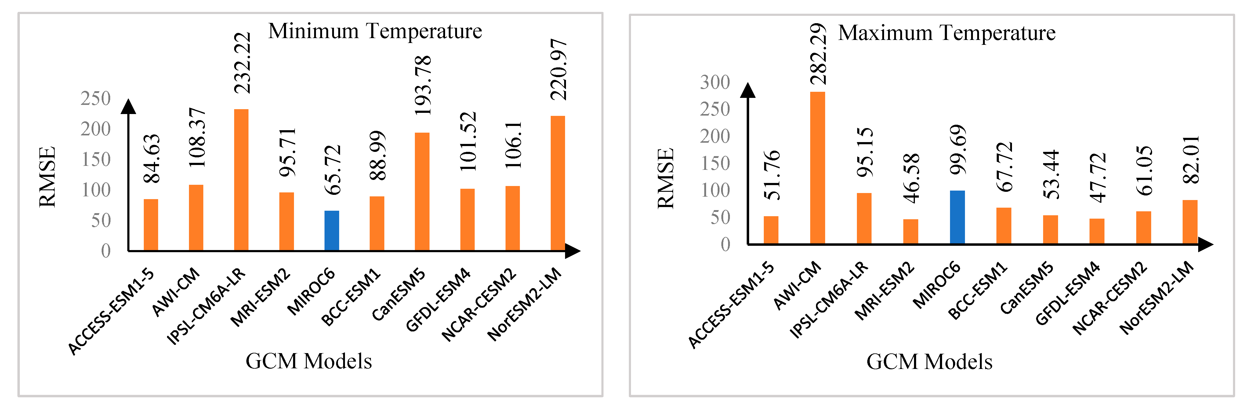
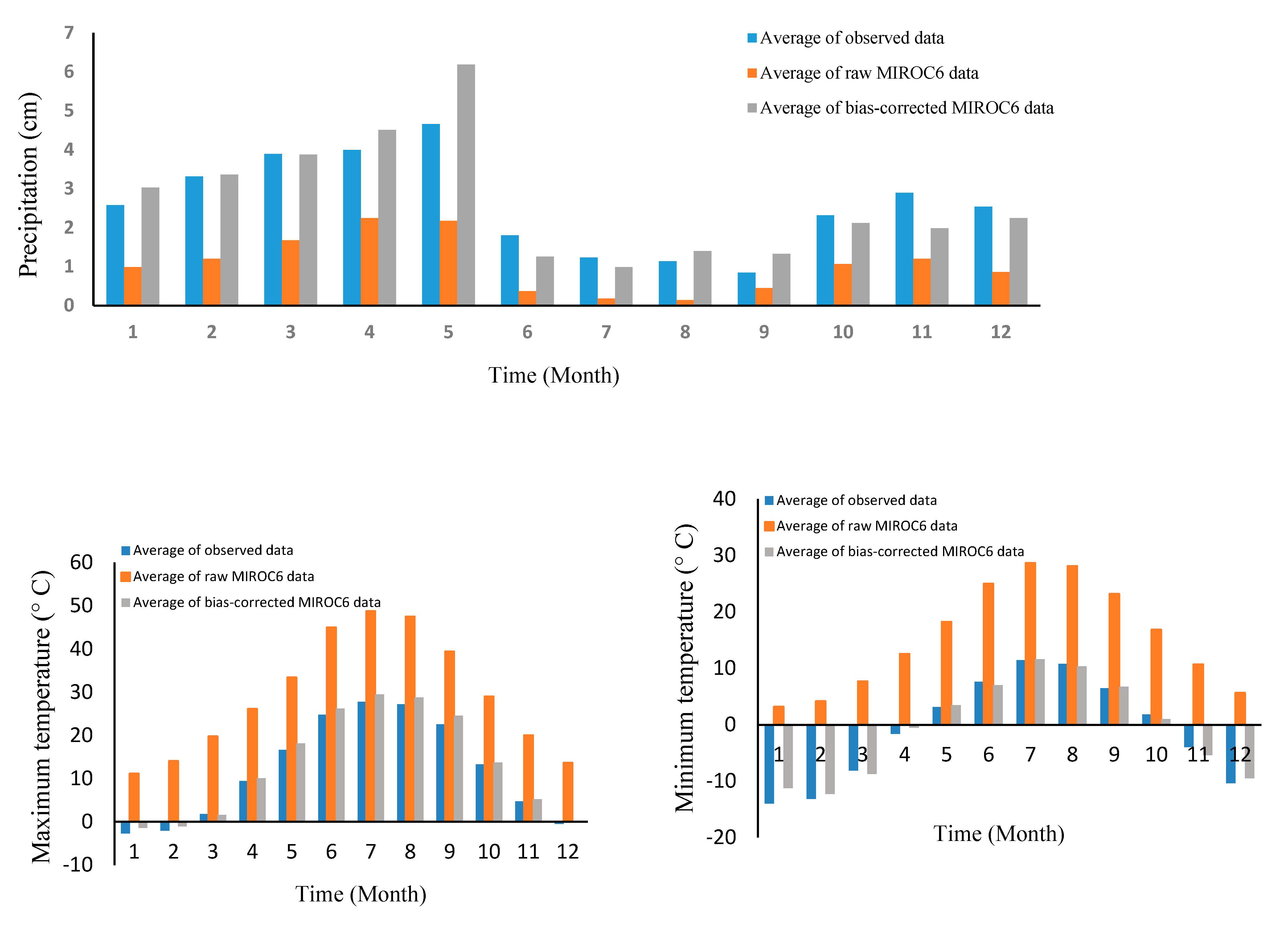
3.2. Climate Modeling
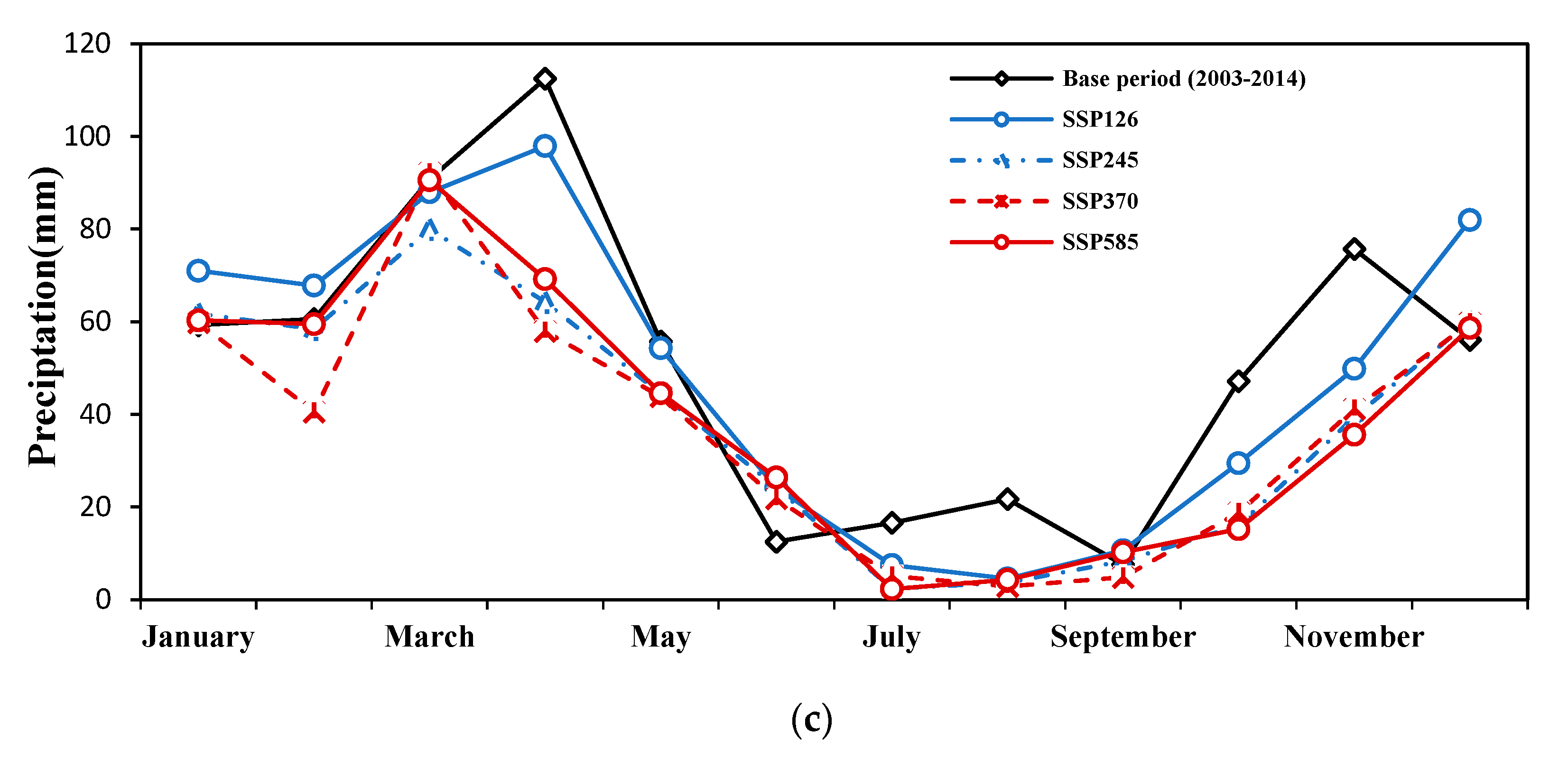
3.3. Future Projection of Temperature and Precipitation
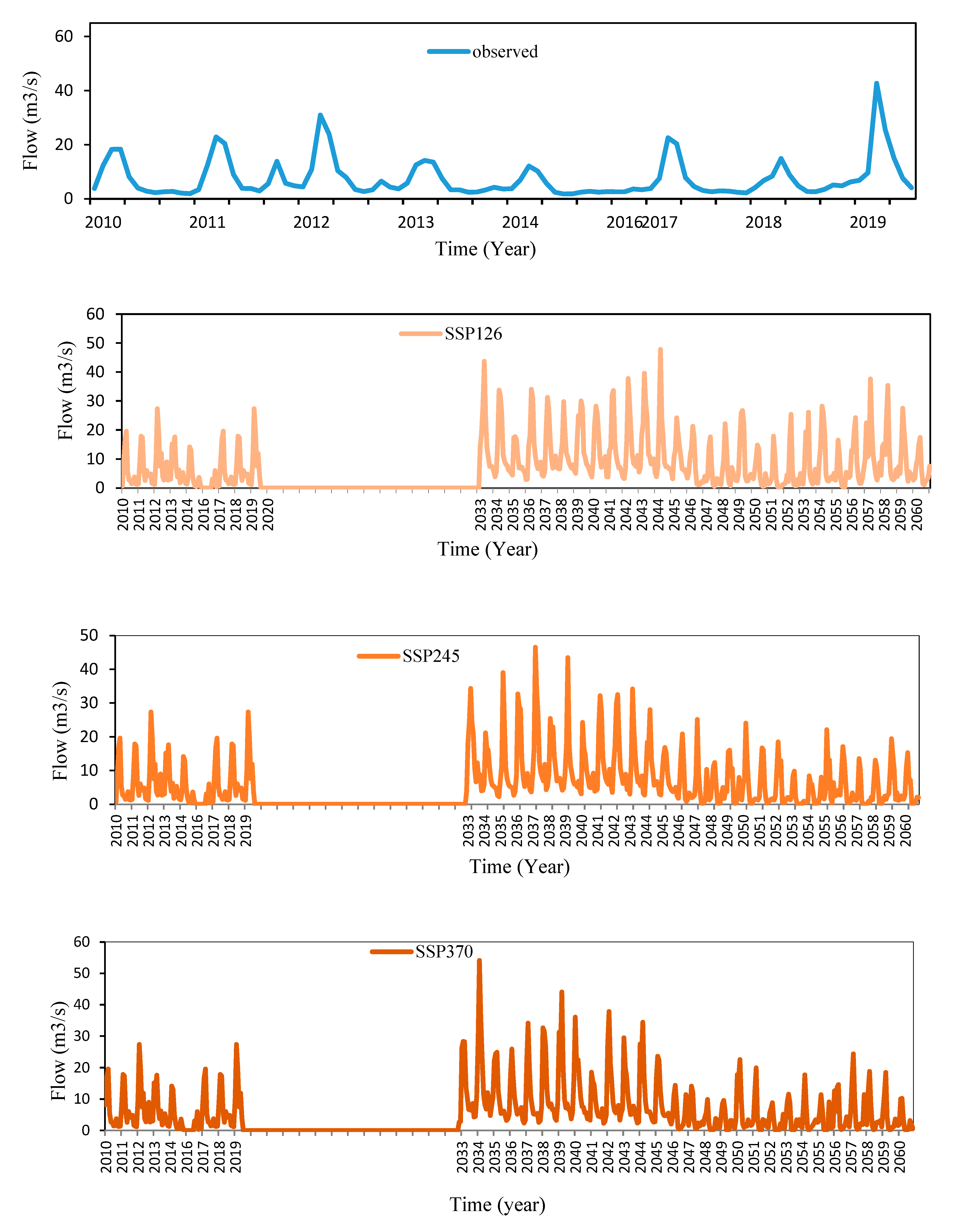
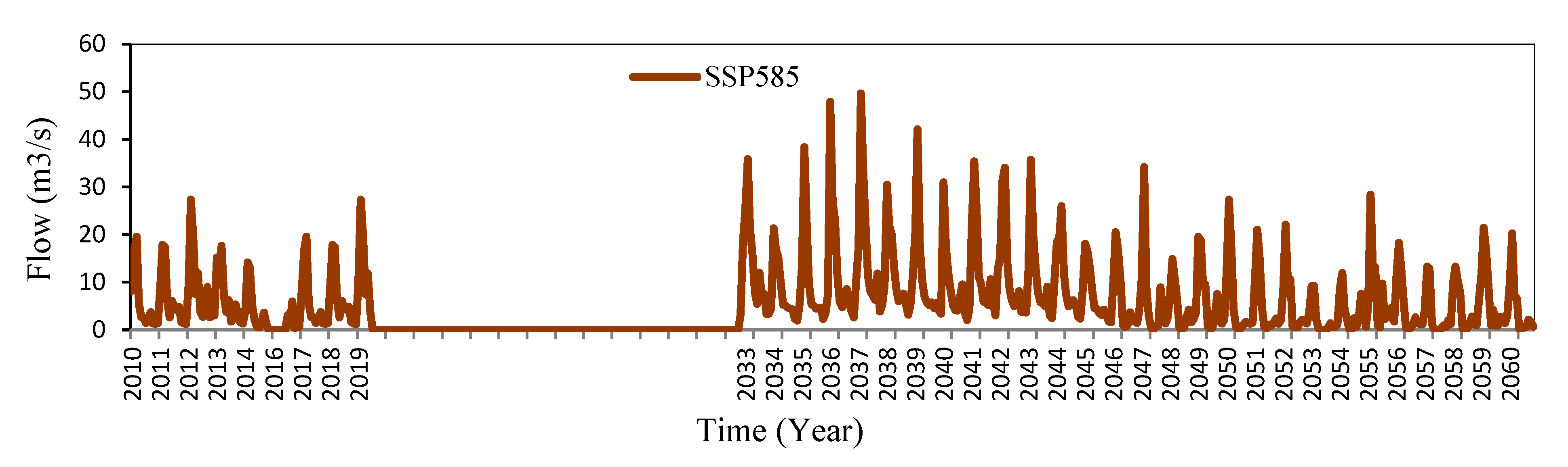
3.4. Projection of Future Discharge
3.5. Limitations and Suggestions
4. Discussion
4.1. Interpreting Research Results while Considering Results of Previous Studies
4.2. Potential Threats of Climate Change
5. Conclusions
Author Contributions
Funding
Institutional Review Board Statement
Informed Consent Statement
Data Availability Statement
Conflicts of Interest
References
- Bhatt, I.; Huggel, C.; Insarov, G.; Morecroft, M.; Muccione, V.; Prakash, A. Summary of Mountain. Intergovernmental Panel on Climate Change Sixth Assessment Report Working Group II Report—Climate Change 2022: Impacts, Adaptation and Vulnerability; IPCC: Geneva, Switzerland, 2022. [Google Scholar]
- Alavi Naini, A.; Malek Mohamadi, B. The effects of global warming on extreme rainfall to floods with different return periods (case study: Jajroud watershed). Sci. Q. J. 2020, 29, 241–246. [Google Scholar]
- Mohseni-Bandpei, A.; Nasseri, M.; Rafiee, M.; Eslamizadeh, M.; Hashempour, Y. Impact of Climate Change on Organic Carbon Removal Efficiency in Jajrood Catchment: From Dam to Water Treatment Plant. J. Maz. Univ. Med. Sci. 2020, 30, 81–95. [Google Scholar]
- IPCC. Climate Change 2007: The Physical Science Basis. Impacts, Adaptation and Vulnerability. Contribution of Working Group II to the Fourth Assessment Report of the Intergovernmental Panel on Climate Change; Cambridge University Press: Cambridge, UK, 2007; 996p.
- IPCC. Summary of Policy Makers Intergovernmental Panel on Climate Change Fifth Assessment Report Working Group IReport—Climate Change 2013: Natural Science Foundation; Stocker, T.F., Qin Dahe, G., Plattner, K., Tignor, M., Allen, S.K., Boschung, J., Nauels, A., Xia, Y., Bex, V., Midgley, P.M., Eds.; University of Cambridge Press: Cambridge, UK; New York, NY, USA, 2013.
- Gebrechorkos, S.; Bernhofer, C.; Hülsmann, S. Climate change impact assessment on the hydrology of a large river basin in Ethiopia using a local-scale climate modelling approach. Sci. Total Environ. 2020, 742, 140504. [Google Scholar] [CrossRef] [PubMed]
- Zhang, X.; Xu, Y.-P.; Fu, G. Uncertainties in SWAT extreme flow simulation under climate change. J. Hydrol. 2014, 515, 205–222. [Google Scholar] [CrossRef]
- Wen, K.; Gao, B.; Li, M. Quantifying the Impact of Future climate change on Runoff in the Amur River basin using a distributed hydrological model and CMIP6 GCM projections. Atmosphere 2021, 12, 1560. [Google Scholar] [CrossRef]
- Hakala, K.; Addor, N.; Teutschbein, C.; Vis, M.; Dakhlaoui, H.; Seibert, J. Hydrological modeling of climate change impacts. J. Sci. Technol. Soc. 2020. [Google Scholar] [CrossRef]
- Bhatta, B.; Shrestha, S.; Shrestha, P.; Talchabhadel, R. Evaluation and application of a SWAT model to assess the climate change impact on the hydrology of the Himalayan River Basin. Catena 2019, 181, 104082. [Google Scholar] [CrossRef]
- Tian, P.; Lu, H.; Feng, W.; Guan, Y.; Xue, Y. Large decrease in streamflow and sediment load of Qinghai-Tibetan Plateau driven by future climate change: A case study in Lhasa River Basin. Catena 2019, 187, 104340. [Google Scholar] [CrossRef]
- Abtahi, S.M. Investigating the paleoclimate of Jajrood watershed use of glacial evidence Persian. J. Geogr. Explor. Desert Areas 2013, 1, 185–201. [Google Scholar]
- Khosravi, Y.; Pari-Zanganeh, A.H.; Karimian, V.; Doustkamian, M.; Shiri, A. Analysis of climatic zoning and investigation of the effects of climatic elements on the discharge of the Jajrood river watershed Persian. J. Rain Pool Surf. Syst. 2019, 6, 19. [Google Scholar]
- Gusain, A.; Ghosh, S.; Karmakar, S. Added value of CMIP6 over CMIP5 models in simulating Indian summer monsoon rainfall. Atmos. Res. 2020, 232, 104680. [Google Scholar] [CrossRef]
- Maurer, E.P.; Hidalgo, H.G. Utility of daily vs. monthly large-scale climate data: An intercomparison of two statistical downscaling methods. Hydrol. Earth Syst. Sci. 2008, 12, 551–563. [Google Scholar] [CrossRef]
- IPCC. Summary of Future Global Climate: Scenario-Based Projections and Near-Term Information. Intergovernmental Panel on Climate Change Sixth Assessment Report Working Group I Report—Climate Change 2021: The Physical Science Basis; IPCC: Geneva, Switzerland, 2021.
- Naseri, E.; Massah Bavani, A.R.; Saadi, T.; Javadi, S. Detection and Attribution of Climate Change Effects on Inflow to Karaj Dam in the Past Periods Persian. J. Iran-Water Resour. Res. 2020, 16, 306–321. [Google Scholar]
- Gutmann, E.D.; Rasmussen, R.M.; Liu, C.; Ikeda, K.; Gochis, D.J.; Clark, M.P.; Dudhia, J.; Thompson, G. A Comparison of statistical and dynamical downscaling of winter precipitation over complex terrain. J. Clim. 2012, 25, 262–281. [Google Scholar] [CrossRef]
- Li, H.; Sheffield, J.; Wood, E.F. Bias correction of monthly precipitation and temperature fields from Intergovernmental Panel on Climate Change AR4 models using equidistant quantile matching. J. Geophys. Res. 2010, 115, D10101. [Google Scholar] [CrossRef]
- Xue, Y.; Janjic, Z.; Dudhia, J.; Vasic, R.; De Sales, F. A review on regional dynamical downscaling in intrapersonal to seasonal simulation/prediction and major factors that affect downscaling ability. Atmos. Res. 2014, 147, 68–85. [Google Scholar] [CrossRef]
- Salvi, K.; Kannan, S.; Ghosh, S. High-resolution multisite daily rainfall projections in India with statistical downscaling for climate change impacts assessment. J. Geophys. Res. Atmos. 2013, 118, 3557–3578. [Google Scholar] [CrossRef]
- Gebrechorkos, S.H.; Bernhofer, C.; Hülsmann, S. Impacts of projected change in climate on water balance in basins of East Africa. Sci. Total Environ. 2019, 682, 160–170. [Google Scholar] [CrossRef]
- Lutz, A.F.; ter Maat, H.W.; Biemans, H.; Shrestha, A.B.; Wester, P.; Immerzeel, W.W. Selecting representative climate models for climate change impact studies: An advanced envelope-based selection approach. Int. J. Clim. 2016, 36, 3988–4005. [Google Scholar] [CrossRef]
- Dunn, S.M.; Brown, I.; Sample, J.; Post, H. Relationships between climate, water resources, land use and diffuse pollution and the significance of uncertainty in climate change. J. Hydrol. 2012, 434–435, 19–35. [Google Scholar] [CrossRef]
- Osmani, H.; Motamedvaziri, B.; Moeni, A. Simulation of discharge, calibration and validation of SWAT model case study: Tehran Latyan dam upstream Persian. J. Watershed Eng. Manag. 2013, 5, 134–143. [Google Scholar]
- Arnold, J.G.; Srinivasan, R.; Muttiah, S.R.; Williams, J.R. Large area hydrologic modeling and assessment part I. Model development. JAWRA J. Am. Water Resour. Assoc. 1998, 34, 73–89. [Google Scholar] [CrossRef]
- Zakizadeh, H.; Ahmadi, H.; Zehtabian, G.; Moeini, A.; Moghaddamnia, A. A novel study of SWAT and ANN models for runoff simulation with application on dataset of metrological stations. Phys. Chem. Earth Parts A/B/C 2020, 120, 102899. [Google Scholar] [CrossRef]
- Marin, M.; Clinciu, I.; Tudose, N.C.; Ungurean, C.; Adorjani, A.; Mihalache, A.L.; Davidescu, A.A.; Davidesco, O.; Dinca, L.; Cacovean, H. Assessing the vulnerability of water resources in the context of climate changes in a small forested watershed using SWAT: A review. Environ. Res. 2020, 184, 109330. [Google Scholar] [CrossRef] [PubMed]
- Jimeno-seaz, P.; Martines-Espana, R.; Casali, J.; Perez-sanches, J.; Senet-Aparicio, J. A comparison of performance of SWAT and machine learning models for predicting sediment load in a forested Basin, Northern Spain. Catena 2020, 212, 105953. [Google Scholar] [CrossRef]
- Meaurio, M.; Zabaleta, A.; Uriarte, J.A.; Srinivasan, R.; Antigüedad, I. Evaluation of SWAT models performance to simulate streamflow spatial origin. The case of a small forested watershed. J. Hydrol. 2015, 525, 326–334. [Google Scholar] [CrossRef]
- Khalilian, S.; Shahvari, N. A SWAT Evaluation of the Effects of Climate Change on Renewable Water Resources in Salt Lake Sub-Basin, Iran. AgriEngineering 2018, 1, 44–57. [Google Scholar] [CrossRef]
- Arnold, J.G.; Kiniry, J.R.; Srinivasan, R.; Williams, J.R.; Haney, E.B.; Neitsch, S.L. Soil and Water Assessment Tool Input/Output File Documentation, Version 2009; Texas Water Resources Institute Technical Report; Texas Water Resources Institute: College Station, TX, USA, 2011; p. 365. [Google Scholar]
- Baffaut, C.; Sadler, E.J.; Ghidey, F.; Anderson, S.H. Long-term agroecosystem research in the central mississippi river basin: SWAT simulation of flow and water quality in the goodwater creek experimental watershed. J. Environ. Qual. 2015, 44, 84–96. [Google Scholar] [CrossRef]
- Singh, V.; Bankar, N.; Salunkhe, S.S.; Bera, A.K.; Sharma, J.R. Hydrological stream flow modelling on Tungabhadra catchment: Parameterization and uncertainty analysis using SWAT CUP. Curr. Sci. 2013, 104, 1187–1199. [Google Scholar]
- FAO. The State of Food Insecurity in the World (SOFI); Food and Agricultural Organization of the United Nations: Rome, Italy; World Bank: Washington, DC, USA, 2014. [Google Scholar]
- Arnold, J.; Moriasi, D.; Gassman, P.; Abbaspour, K.; White, M.; Srinivasan, R.; Santhi, C.; Harmel, R.; van Griensven, A.; Van Liew, M.; et al. SWAT: Model use, calibration, and validation. Trans. ASABE 2012, 55, 1491–1508. [Google Scholar] [CrossRef]
- Abbaspour, K.C.; Yang, J.; Maximov, I.; Siber, R.; Bogner, K.; Mieleitner, J.; Zobrist, J.; Srinivasan, R. Modelling hydrology and water quality in the pre-alpine/alpine Thur watershed using SWAT. J. Hydrol. 2007, 333, 413–430. [Google Scholar] [CrossRef]
- Wu, H.; Chen, B. Evaluating uncertainty estimates in distributed hydrological modeling for the Wenjing River watershed in China by GLUE, SUFI-2, and Parasol methods. Ecol. Eng. 2015, 76, 110–121. [Google Scholar] [CrossRef]
- Parajuli, P.B.; Jayakody, P.; Ouyang, Y. Evaluation of using remote sensing evapotranspiration data in SWAT. Water Resour. Manag. 2018, 32, 985–996. [Google Scholar] [CrossRef]
- Park, J.-Y.; Yu, Y.-S.; Hwang, S.-J.; Kim, C.; Kim, S.-J. SWAT modeling of best management practices for Chungju dam watershed in South Korea under future climate change scenarios. Paddy Water Environ. 2014, 12, 65–75. [Google Scholar] [CrossRef]
- Abbaspour, K.C.; Rouholahnejad, E.; Vaghefi, S.; Srinivasan, R.; Yang, H.; Kløve, B. A continental-scale hydrology and water quality model for Europe: Calibration and uncertainty of a high-resolution large-scale SWAT model. J. Hydrol. 2015, 524, 733–752. [Google Scholar] [CrossRef]
- Nash, J.E.; Sutcliffe, J.V. River flow forecasting through conceptual Models part I—A discussion of principles. J. Hydrol. 1970, 10, 282–290. [Google Scholar] [CrossRef]
- Ha, L.T.; Bastiaanssen, W.G.; van Griensven, A.; van Dijk, A.I.; Senay, G.B. SWAT-CUP for calibration of spatially distributed hydrological processes and ecosystem services in a Vietnamese river basin using remote sensing. Hydrol. Earth Syst. Sci. Discuss. 2017, 1–35. [Google Scholar] [CrossRef]
- Moriasi, D.; Arnold, J.; van Liew, M.; Bingner, R.; Harmel, R.; Veith, T. Model evaluation guidelines for systematic quantification of accuracy in watershed simulations. Trans. ASABE 2007, 50, 885–900. [Google Scholar] [CrossRef]
- Nourani, V. Reply to comment on ‘Nourani V, Mogaddam AA, Nadiri AO. 2008. An ANN-based model for spatiotemporal groundwater level forecasting. Hydrological Processes 22: 5054–5066’. Hydrol. Process. 2010, 24, 370–371. [Google Scholar] [CrossRef]
- Riahi, K.; Van Vuuren, D.P.; Kriegler, E.; Edmonds, J.; O’Neill, B.C.; Fujimori, S.; Bauer, N.; Calvin, K.; Dellink, R.; Fricko, O.; et al. The shared socioeconomic pathways and their energy, land use, and greenhouse gas emissions implications: An overview. Glob. Environ. Change 2017, 42, 153–168. [Google Scholar] [CrossRef]
- Mehrotra, R.; Johnson, F.; Sharma, A. A software toolkit for correction systematic biases in climate model simulations. Environ. Model. Softw. 2018, 104, 130–152. [Google Scholar] [CrossRef]
- Mehrotra, R.; Sharma, A. A multivariate quantile-matching bias correction approach with auto- and cross-dependence across multiple time scales: Implications for downscaling. J. Clim. 2016, 29, 3519–3539. [Google Scholar] [CrossRef]
- Teutschbein, C.; Seibert, J. Is bias correction of regional climate model (RCM) simulations possible for non-stationary conditions? Hydrol. Earth Syst. Sci. 2013, 17, 5061–5077. [Google Scholar] [CrossRef]
- Mehrotra, R.; Sharma, A. An improved standardization procedure to remove systematic low frequency variability biases in GCM simulations. Water Resour. Res. 2012, 48, 1–8. [Google Scholar] [CrossRef]
- Johnson, F.; Sharma, A. A nesting model for bias correction of variability at multiple time scales in general circulation model precipitation simulations. J. Water Resour. Res. 2012, 48, 1–16. [Google Scholar] [CrossRef]
- Wilby, R.L.; Charles, S.P.; Zorita, E.; Timbal, B.; Whetton, P.; Mearns, L.O. Guidelines for Use of Climate Scenarios Developed from Statistical Downscaling Methods; IPCC Task Group on Scenarios for Climate Impact Assessment: Geneva, Switzerland, 2004; 27p. [Google Scholar]
- Mehrotra, R.; Sharma, A. Correcting for systematic biases in multiple raw GCM variables across a range of timescales. J. Hydrol. 2015, 520, 214–223. [Google Scholar] [CrossRef]
- Fan, G.; Sarabandi, A.; Yaghoobzadeh, M. Evaluating the climate change effects on temperature, precipitation and evapotranspiration in eastern Iran using CMIP5. Water Supply 2021, 21, 4316–4327. [Google Scholar] [CrossRef]
- Hoshmand Kouchi, D.; Esmaili, K.; Farid Hosseini, A.; Sanaeinejad, S.H.; Khalili, D. Simulation of climate change impacts using fifth assessment report models under RCP scenarios on water resources in the upper basin of salman farsi dam. Iran. J. Irrig. Drain. 2018, 13, 243–258. [Google Scholar]
- Abbaspour, K.C.; Faramarzi, M.; Ghasemi, S.S.; Yang, H. Assessing the impact of climate change on water resources in Iran. Water Resour. Res. 2009, 45, W10434. [Google Scholar] [CrossRef]
- Fallah Kalaki, M.; Shokri Kuchak, V.; Ramezani Etedali, H. Simulating the effects of climate change on run off using the CMIP6 and CMIP5 climate models by swat hydrological model (case study: Tashk-Bakhtegan basin). J. Iran Water Resour. Res. 2021, 17, 345–359. [Google Scholar]
- Riahi, K.; Schaeffer, R. Climate Change 2022, IPCC AR6 WG III Mitigation Pathways Compatible with Long-Term Goals; IPCC: Geneva, Switzerland, 2022. [Google Scholar]
- Mahdian, M.; Hosseinzadeh, M.; Siadatmousavi, S.M.; Chalipa, Z.; Dalavar, M.; Guo, M.; Abolfathi, S.; Noori, R. Modelling impacts of climate change and anthropogenic activities on inflows and sediment loads of wetlands: Case study of the Anzali wetland. Sci. Rep. 2023, 13, 5399. [Google Scholar] [CrossRef] [PubMed]
- Abbaszadeh, M.; Bazrafshan, O.; Mahdavi, R.; Sardooi, E.R.; Jamshidi, S. Modeling Future Hydrological Characteristics Based on Land Use/Land Cover and Climate Changes Using the SWAT Model. Water Resour. Manag. 2023, 37, 1–18. [Google Scholar] [CrossRef]


| Name | Base Period | Latitude | Longitude | Elevation (m) | Precipitation (mm/y) |
|---|---|---|---|---|---|
| p-Emmame | 2005–2019 | 35.91 | 51.58 | 2248 | 587 |
| p-Polur | 2005–2019 | 35.85 | 52.06 | 2273 | 609 |
| p-Abbaspour | 2005–2019 | 35.74 | 51.58 | 1482 | 336 |
| p-Kiga | 2005–2019 | 35.86 | 51.31 | 2009 | 690 |
| p-Latyan | 2005–2019 | 35.78 | 51.68 | 1563 | 402 |
| Sub-Watershed | Station | River | Coordinates | Elevation (m) | Area (km2) | |
|---|---|---|---|---|---|---|
| UTM-Y | UTM-X | |||||
| 15 | Bagh Tange | Emame | 3973014 | 552641 | 2210 | 18.69 |
| 19 | Kamarkhani | Emame | 3967443 | 548159 | 1890 | 36.85 |
| 22 | Roudak | Jajrood | 3966557 | 550717 | 1710 | 419.9 |
| 28 | Lavarak | Ali abad | 3962250 | 563250 | 1600 | 97.12 |
| 23 | Naroun | Afje | 3965750 | 560000 | 1750 | 28.83 |
| 24 | Najar kola | Golandouk | 3965250 | 557500 | 1700 | 57.29 |
| No. | Parameters | Definition |
|---|---|---|
| 1 | GW_Delay.gw | Groundwater delay |
| 2 | GWQMN.gw | Threshold in the shallow aquifer for return flow to occur |
| 3 | GW_Revap.gw | Groundwater “revap” coefficient |
| 4 | SHALLST.gw | Initial depth of water in the shallow aquifer |
| 5 | ALPHA_BF.gw | Base flow alpha factor (days) |
| 6 | REVAPMN.gw | Threshold in the shallow aquifer for “revap” to occur |
| 7 | RCHRG_DP.gw | Deep aquifer percolation fraction |
| 8 | CN2.mgt | SCS stream flow curve number |
| 9 | ADJ_PKR.bsn | Peak rate adjustment factor for sediment routing in the sub basin |
| 10 | MSK-CO1.bsn | Muskingum channel routing (coefficient for normal flow routing) |
| 11 | MSK-CO2.bsn | Muskingum channel routing (coefficient for low flow routing) |
| 12 | MSK-X.bsn | Muskingum channel routing (weighting factor) |
| 14 | SOL_AWC (relative test).bsn | Available water capacity of the soil layer |
| 15 | SOL_K (relative test).bsn | Saturated hydraulic conductivity |
| 16 | SOL_BD(1).bsn | Moist bulk density of first soil layer (Mg/m3) |
| 17 | SOL_ALB.bsn | Soil albedo (dimensionless) |
| 18 | SFTMP.bsn | Snowfall temperature |
| 19 | SMTMP.bsn | Snowmelt base temperature |
| 20 | SMFMX.bsn | Maximum melt rate for snow during year (summer solstice) |
| 21 | SMFMN.bsn | Minimum melt rate for snow during year (winter solstice) |
| 22 | TIMP.bsn | Snowpack temperature lag factor |
| 23 | SNO_SUB.bsn | Initial snow water content |
| 24 | SNOWCOVMX.bsn | Snow water content that corresponds to 100% snow cover |
| 25 | SNOW50COV.bsn | Snow water equivalent that corresponds to 50% snow cover |
| 26 | Plaps.sub | Precipitation lapse rate |
| 27 | Tlaps.sub | Temperature lapse rate |
| 28 | ESCO.hru | Soil evaporation compensation factor |
| Parameter Name | Sensitivity Ranks | Range Update | File | Min. Value | Max. Value | Fitted Value |
|---|---|---|---|---|---|---|
| SNO50COV | 1 | V | .bsn | 0 | 500 | 471. |
| ESCO | 2 | V | .hru | −0.2 | 0.2 | 0.157800 |
| RCHRG_DP | 3 | V | .gw | 0 | 1 | 0.003000 |
| GWQMN | 4 | V | .gw | 0 | 5000 | 2945.000000 |
| PLAPS | 5 | V | .sub | 0 | 400 | 68.500000 |
| CN2 | 6 | V | .mgt | −0.2 | 0.2 | 0.148200 |
| OV_N | 7 | V | .hru | −0.2 | 0.2 | 0.127800 |
| MSK_CO1 | 8 | V | .bsn | 0.0 | 10.0 | 1.745000 |
| Parameter | Indices | Roudak Station | |
|---|---|---|---|
| Calibration (2010–2014) | Validation (2016–2019) | ||
| Flow | R2 | 0.85 | 0.74 |
| PBIAS | 14.4 | 15 | |
Disclaimer/Publisher’s Note: The statements, opinions and data contained in all publications are solely those of the individual author(s) and contributor(s) and not of MDPI and/or the editor(s). MDPI and/or the editor(s) disclaim responsibility for any injury to people or property resulting from any ideas, methods, instructions or products referred to in the content. |
© 2023 by the authors. Licensee MDPI, Basel, Switzerland. This article is an open access article distributed under the terms and conditions of the Creative Commons Attribution (CC BY) license (https://creativecommons.org/licenses/by/4.0/).
Share and Cite
Najimi, F.; Aminnejad, B.; Nourani, V. Assessment of Climate Change’s Impact on Flow Quantity of the Mountainous Watershed of the Jajrood River in Iran Using Hydroclimatic Models. Sustainability 2023, 15, 15875. https://doi.org/10.3390/su152215875
Najimi F, Aminnejad B, Nourani V. Assessment of Climate Change’s Impact on Flow Quantity of the Mountainous Watershed of the Jajrood River in Iran Using Hydroclimatic Models. Sustainability. 2023; 15(22):15875. https://doi.org/10.3390/su152215875
Chicago/Turabian StyleNajimi, Farzaneh, Babak Aminnejad, and Vahid Nourani. 2023. "Assessment of Climate Change’s Impact on Flow Quantity of the Mountainous Watershed of the Jajrood River in Iran Using Hydroclimatic Models" Sustainability 15, no. 22: 15875. https://doi.org/10.3390/su152215875
APA StyleNajimi, F., Aminnejad, B., & Nourani, V. (2023). Assessment of Climate Change’s Impact on Flow Quantity of the Mountainous Watershed of the Jajrood River in Iran Using Hydroclimatic Models. Sustainability, 15(22), 15875. https://doi.org/10.3390/su152215875