Relationships between Thermal Environment and Air Pollution of Seoul’s 25 Districts Using Vector Autoregressive Granger Causality

Abstract

Rising temperatures and heightened air pollution are widespread across many parts of the world today. Despite some initial attempts for analysis, the intricate interconnection between the two still requires further investigation. This study focuses on Seoul, South Korea, by adopting vector-autoregressive-based Granger causality tests to unravel the nuances of these relationships at the district level. While bidirectional Granger causality links between temperature and urban heat island intensity, as well as between PM₁₀ concentration and urban pollution island intensity, are found in many cases, our findings reveal diverse causal relationships that are evident in the districts. These findings underscore the necessity for evidence-based strategies to guide planners and policymakers in addressing the challenges of rising temperatures and air pollution in urban areas.

1. Introduction

Of the many environmental challenges South Korea faces today, rising temperatures and increasing air pollution levels are widely perceived by locals as one of the most critical [1,2]. The country’s overall temperature rose by up to 2.6 times faster than the global average over the past century [3], and air pollution levels of most of the country’s cities, usually represented among the locals by the concentration of particulate matter 10 μm or less in diameter (PM₁₀), frequently exceed the World Health Organization (WHO)’s guidelines and remain higher than those of major global cities [4,5,6].

The consequential impacts of these challenges are tangibly evident. The country’s rising temperatures, especially during hot seasons, inflate the demand and consumption of energy [7,8], increase heat-related illnesses and deaths [9,10,11], and put its ecosystem and natural resources at higher risk. The high concentrations of PM₁₀ exacerbate respiratory, cardiovascular, and skin diseases [12] and increase premature deaths [13].

To generate policy measures to tackle rising temperatures and air pollution levels, research has been identifying each of their causes. First, warming is caused by excessive emission of greenhouse gases, produced naturally or by anthropogenic activities, into the Earth’s atmosphere. They encompass reliance on fossil fuels for transportation, heating, cooling, and power generation, alongside urban land transformations catering to burgeoning infrastructural demands, particularly within densely populated cities [14,15,16,17]. Second, rising air pollution levels, especially the PM₁₀ concentrations, highly depend on anthropogenic sources, including automobiles, industrial facilities, power plants, and buildings, in addition to natural sources like volcano eruptions, wildfires, and the decomposition of organic substances [18,19,20].

Notably, a larger body of literature finds that temperatures and concentrations of PM₁₀ operate as a cause for each other in cities using statistical approaches in which usually independent and dependent variables are fixed. They identify temperature as a statistically significant or highly important explanatory variable when predicting PM₁₀ concentrations [21,22,23,24,25,26,27], as heat increases energy use, thereby emitting more air pollutants and generating secondary aerosols in the atmosphere [28,29,30]. Another substantial body presents evidence that particulates induce discernible temperature fluctuations, often facilitated through radiative forcing mechanisms [31,32,33,34].

To address thermal environment and air pollution levels at the same time, some researchers use correlations to explain the relationship [35,36,37]. One German study, using an attribution method, finds that a highly complex interaction exists between temperatures and PM₁₀ concentrations, as the former intensify turbulence mixing and the latter affect radiation transfer processes at the same time [38]. A study from China adopts Granger causality tests to reveal the intricate interactions between fine particles and urban heat islands at seasonal, monthly, and daily scales [39]. Another study from northeastern United States develops a vulnerability index to address their interaction [40]. However, it is difficult to find studies that attempt to explain the intricate causal relationships among multiple time series variables.

These studies commonly suggest that the relationship between temperatures and PM₁₀ concentrations manifests in diverse ways. Yet, they also clearly demonstrate that it is difficult to converge to a firm agreement on the causal relationship between the two. Studies remark that existence, directions, and strengths of the relationships may significantly differ by spatial and temporal conditions set for each study and strongly call for further investigation across diverse contexts [35,39,41].

We look into Seoul, South Korea, which stands as the country’s capital city and also as one of the fastest warming and air-polluted cities in Far East Asia. We unravel the intricate causal relationships between the thermal environment and air pollution in Seoul’s 25 administrative districts, which form the bedrock of the city’s local policymaking. More specifically, we investigate temperatures and PM₁₀ concentrations, as well as urban heat island intensity (UHII) and urban pollution island intensity (UPII), to yield deeper insights. We use data collected at each of the 25 districts’ weather and air monitoring stations from 1 January 2015 to 31 December 2019, the most recent five-year period prior to the outbreak of COVID-19, and employ a vector autoregressive (VAR)-based Granger causality test. Our findings may help to provide a strategic framework for crafting effective and targeted interventions tailored for each district. They can also serve as a valuable reference for urban regions worldwide that are grappling with similar challenges.

2. Materials and Methods

2.1. Case Context

As previously mentioned, Seoul (37°33′36″ N 126°59′24″ E) has long been experiencing rapid warming and a high concentration of PM₁₀. Figure 1 reports that its annual average temperatures remained generally below 12 °C in the 1960s but rose sharply since then and now nears 14 °C. This corresponds to an increase rate of 0.3 °C per decade, which is more than twice the global average of 0.18 °C per decade since 1981 [42]. Figure 2 shows Seoul’s monthly PM₁₀ concentration trends since 2015. Although there has been a gradual decline over time with seasonal fluctuations and a significant drop since early 2020, the concentrations still remain well above the WHO’s guidelines, 15 μg/m³. While the concentrations of most other major air pollutants like sulfur dioxide, nitrogen dioxide, carbon monoxide, and ozone remain low, PM₁₀ stands out as a significant concern for local researchers and policymakers and is regarded as one of the few pollutants that still requires substantial improvement [43,44].

2.2. Variables and Data

Seoul, for a better accommodation of its 9.4 million residents and 5.7 million jobs on approximately 605 square kilometers of land, subdivides itself into 25 districts mostly based on population, as Figure 3 illustrates. Since the mid-1900s, Seoul’s neighborhoods have typically expanded in a way that broadly adheres to district borders. Today, districts ensure a relatively even provision of public service throughout Seoul and actively play a central role in developing significant planning and policy decisions. For this reason, we carry out analysis at the district level.

Our variables primarily fall into two categories: thermal environment and air pollution. For the former, we employ daily average temperatures and UHII, which is measured by the difference between the urban air temperature and the background rural temperature [45,46]. For the latter, we utilize daily average PM₁₀ concentrations and UPII, which is determined by the difference in the concentration between urban areas and rural areas [41,47].

Data for the two thermal environment variables are sourced from the 29 weather stations situated in Seoul, as presented in Figure 4. There is at least one weather station in each district that makes it possible to assign relevant data to each district. Of the 29, 2 stations were excluded since they sit on high mountains or along rivers. For the two districts with two weather stations, we use averages of the two readings. We downloaded relevant data from the Open Met Data Portal (https://data.kma.go.kr/, accessed on 29 September 2023) of the Korea Meteorological Administration. Likewise, data for the two air pollution variables originate from the city’s 40 air quality monitoring stations, also illustrated in Figure 4, ensuring representation of at least 1 station in each district. We use averages for districts with two stations. Relevant data are downloaded from the Seoul Metropolitan Government’ Seoul Atmospheric Environment Information (https://cleanair.seoul.go.kr/, accessed on 29 September 2023).

While constructing the time series for daily average temperatures and PM₁₀ concentrations, we encountered missing data points, constituting about 3% of the dataset. With this relatively minor percentage, we opted for linear interpolation as our preferred method, predicting values using neighboring data points.

By drawing from prior research [48,49,50], we compute the UHII and UPII by quantifying the difference between the average measurements taken within the confines of Seoul and those obtained at a reference location situated outside the city limits. We use the following formulae to calculate UHII and UPII:

$$UHI{I}_i={\overline{T}}_i-{\overline{T}}_r$$

(1)

$$UPI{I}_i={\overline{P}}_i-{\overline{P}}_r$$

(2)

where $UHI{I}_i$ is the UHII of location $i$, ${\overline{T}}_i$ is the average temperature of location $i$, ${\overline{T}}_r$ is the average temperature of the reference point $r$, $UPI{I}_i$ is the UPII of location $i$, ${\overline{P}}_i$ is the average PM₁₀ concentration of location $i$, and ${\overline{P}}_r$ is the average PM₁₀ concentration of the reference point.

From the selection of three potential reference points commonly employed by local researchers—Yangpyeong, Icheon, and Dongducheon—depicted in Figure 4, our preference aligns with Yangpyeong. It receives particular favor due to its distinctly rural characteristics, coupled with its alignment in terms of altitude and latitude with Seoul [51,52,53].

2.3. Analysis

Given the statistical properties of the variables used in this study, we adopt a VAR model approach. It is structured by relating each endogenous variable to the past values of all endogenous variables. This expansion of the univariate autoregressive model results in a vector autoregressive model encompassing multiple time series variables. Originally developed in the 1980s [54], the VAR model offers a straightforward methodology for analyzing and predicting multiple interconnected indicators where all the variables are treated as endogenous [55,56,57]. The VAR model for $p$-order lagged stationary time series data can be expressed as follows:

$$VAR\left(p\right):y_t=v+A_1{y}_{t-1}+\cdots +A_p{y}_{t-p}+u_t$$

(3)

where $v$ is the constant vector, $A_i$ is the regression parameter matrix of independent variables, and $u_t$ is the random error term.

In the context of time series data analysis, the underlying assumption is that the data exhibit stationarity, implying consistent statistical characteristics over time. Nonetheless, numerous real-world datasets deviate from this assumption and display non-stationarity. Such non-stationarity manifests as fluctuations in the mean or variance of the data across time, indicating the presence of a unit root, which can lead to spurious regressions. Therefore, it is necessary to verify whether the time series represents stationarity, which can be confirmed through a unit root test. We use the augmented Dickey–Fuller (ADF) test [58] as it is one of the most favored methods among a few. If a unit root exists, differencing is applied to data in order to remove any sort of stochasticity.

Once it is established that the dataset either possesses stationarity or has been transformed through differencing, the next step involves selecting a suitable lag for analysis. This selection is informed by criteria such as the Akaike information criterion (AIC), the Schwarz Bayesian information criterion (SBIC), and the Hannan–Quinn information criterion (HQIC). In this analysis, we employ all three of these criteria.

Granger causality test [59] is a statistical hypothesis that determines whether one time series is useful for predicting another time series. When the prediction of variable y is improved by including the past value of variable $x$, rather than solely relying on predicting $y$’s current value using its own past values, $x$ is said to Granger-cause $y$. We construct the two following regressions:

$$y_t=\sum _{i=1}^m{\alpha }_i{x}_{t-i}+\sum _{i=1}^n{\beta }_i{y}_{t-i}+u_{1t}$$

(4)

$$x_t=\sum _{i=1}^p{\gamma }_i{x}_{t-i}+\sum _{i=1}^q{\delta }_i{y}_{t-i}+u_{2t}$$

(5)

where $\alpha$, $\beta$, $\gamma$, and $\delta$ are regression coefficients, and $u_t$ is the error terms.

As Figure 5 illustrates, the four variables construct six pairs of variables for six instances for conducting Granger causality tests: (1) daily average temperature and UHII, (2) daily average temperature and daily average PM₁₀ concentration, (3) daily average temperature and UPII, (4) daily average PM₁₀ concentration and UHII, (5) daily average PM₁₀ concentration and UPII, and (6) PM₁₀ concentration and UPII.

In VAR analysis, employing an impulse response function (IRF) is a typical procedure used to identify the influence of modifications in one endogenous variable on another endogenous variable usually in a graphical manner and to observe how the system dynamically reacts to shocks. To account for the immediate impacts of shocks, we employ the orthogonalized impulse response function (IRF), achieved through the utilization of Cholesky decomposition to transform the residual terms to become independent [60,61,62].

Forecast error variance decomposition (FEVD) is a post-analysis step in VAR models. It reveals how much variation in an endogenous variable can be attributed to specific shocks or impulses, separating their distinct effects. Like IRF, it entails orthogonalizing residual terms to determine each variable’s contribution to forecast error variance [63,64].

3. Results

Table 1. Descriptive statistics.

Variable		Unit	Obs.	Mean	Std. Dev
Name	Description
temp	Daily average temperature	°C	45,650	13.5	10.5
uhii	UHII	°C	45,650	0.9	1.4
pm10	Daily average PM10 concentration	μg/m3	45,650	45.4	27.7
upii	UPII	μg/m3	45,650	1.8	11.8

displays the descriptive statistics for the variables under analysis. Among the two thermal environment variables, the daily average temperature exhibits a mean of 13.5 and a standard deviation of 10.5. The mean and standard deviation for UHII are 0.9 and 1.4, respectively. Shifting to the air pollution variables, the mean of daily average PM₁₀ concentration is 45.4, accompanied by a standard deviation of 27.7. The mean UPII is 1.8, with a standard deviation of 11.8.

3.1. Unit Root Test

Table 2. Unit root test results for original data and seasonally differenced data.

District	Original Data				Seasonally Differenced Data
	temp	uhii	pm10	upii	temp	uhii	pm10	upii
Dobong	−2.413	−11.627 ***	−9.368 ***	−11.627 ***	−22.302 ***	−20.416 ***	−20.878 ***	−21.293 ***
Dongdaemun	−2.438	−7.619 ***	−14.201 ***	−10.796 ***	−22.272 ***	−20.919 ***	−20.966 ***	−21.898 ***
Dongjak	−2.337	−8.463 ***	−14.457 ***	−10.289 ***	−22.541 ***	−20.815 ***	−20.751 ***	−21.619 ***
Eunpyeong	−2.428	−8.516 ***	−14.090 ***	−10.172 ***	−22.584 ***	−21.196 ***	−20.400 ***	−20.974 ***
Gangbuk	−2.417	−12.662 ***	−14.403 ***	−9.061 ***	−22.407 ***	−20.949 ***	−20.710 ***	−21.487 ***
Gangdong	−2.370	−8.046 ***	−14.009 ***	−9.761 ***	−22.113 ***	−20.370 ***	−21.114 ***	−22.228 ***
Gangnam	−2.411	−12.029 ***	−14.508 ***	−23.839 ***	−22.470 ***	−21.515 ***	−20.846 ***	−22.123 ***
Gangseo	−2.219	−9.118 ***	−9.158 ***	−9.643 ***	−20.952 ***	−20.973 ***	−20.973 ***	−20.623 ***
Geumcheon	−2.476	−7.666 ***	−14.402 ***	−10.253 ***	−22.559 ***	−21.356 ***	−20.543 ***	−21.628 ***
Guro	−2.537	−8.237 ***	−9.180 ***	−9.967 ***	−22.511 ***	−20.245 ***	−20.592 ***	−21.963 ***
Gwanak	−2.448	−8.413 ***	−14.411 ***	−8.704 ***	−22.529 ***	−21.348 ***	−20.925 ***	−21.952 ***
Gwangjin	−2.372	−10.675 ***	−8.895 ***	−9.328 ***	−22.232 ***	−20.675 ***	−20.744 ***	−22.044 ***
Jongro	−2.427	−9.588 ***	−8.778 ***	−9.547 ***	−22.548 ***	−21.437 ***	−21.080 ***	−22.444 ***
Jung	−2.359	−16.546 ***	−14.963 ***	−9.473 ***	−20.883 ***	−22.264 ***	−20.986 ***	−21.829 ***
Jungrang	−2.413	−15.223 ***	−8.532 ***	−8.867 ***	−22.309 ***	−21.27 ***	−23.393 ***	−21.217 ***
Mapo	−2.464	−15.688 ***	−9.222 ***	−9.873 ***	−22.965 ***	−21.318 ***	−20.889 ***	−21.553 ***
Nowon	−2.301	−24.224 ***	−9.050 ***	−24.444 ***	−22.065 ***	−20.589 ***	−21.022 ***	−21.574 ***
Seocho	−2.391	−8.709 ***	−8.289 ***	−10.111 ***	−22.589 ***	−21.375 ***	−20.641 ***	−21.977 ***
Seodaemun	−2.493	−9.008 ***	−8.97 ***	−10.494 ***	−22.802 ***	−21.484 ***	−20.734 ***	−21.074 ***
Seongbuk	−2.408	−8.203 ***	−9.341 ***	−9.939 ***	−22.437 ***	−21.13 ***	−23.455 ***	−21.763 ***
Seongdong	−2.419	−6.425 ***	−8.231 ***	−9.873 ***	−22.47 ***	−21.224 ***	−20.685 ***	−21.476 ***
Songpa	−2.450	−8.075 ***	−9.627 ***	−9.641 ***	−22.439 ***	−20.473 ***	−20.473 ***	−21.281 ***
Yangcheon	−2.400	−8.516 ***	−14.090 ***	−10.172 ***	−22.584 ***	−21.196 ***	−20.400 ***	−20.974 ***
Yeongdeungpo	−2.428	−8.549 ***	−9.425 ***	−23.188 ***	−22.618 ***	−21.386 ***	−20.934 ***	−21.514 ***
Yongsan	−2.401	−8.837 ***	−9.428 ***	−9.454 ***	−22.547 ***	−21.275 ***	−20.705 ***	−21.684 ***

*** p < 0.001.

shows the ADF test results. Of the four variables in their original forms, we found that the average daily temperature exhibits unit roots in all 25 districts, while the remaining three showed no evidence of unit roots. To eliminate the seasonality present in the temperature data, seasonal differencing was applied to all variables to ensure normality and establish a stable time series for further analysis. As a result, seasonally differenced data successfully pass unit root tests in all cases, as shown in the table.

3.2. Lag Length Selection

We employed AIC, SBIC, and HQIC statistics to ascertain the optimal lag length for each of the 25 districts, taking into consideration that the causal effects may occur gradually and manifest in changes later in time in VAR models. As illustrated in

Table 3. Selected lag lengths for each district.

District	Selected Lag Length (Days)
Dobong	5
Dongdaemun	6
Dongjak	6
Eunpyeong	6
Gangbuk	5
Gangdong	6
Gangnam	6
Gangseo	6
Geumcheon	6
Guro	6
Gwanak	6
Gwangjin	6
Jongro	5
Jung	6
Jungrang	5
Mapo	6
Nowon	6
Seocho	6
Seodaemun	6
Seongbuk	6
Seongdong	6
Songpa	5
Yangcheon	6
Yeongdeungpo	6
Yongsan	6

, five districts, namely Dobong, Gangbuk, Jongro, Jungrang, and Songpa, exhibited a lag length of 5, while that of the remaining twenty was determined to be 6.

3.3. Granger Causality Tests

Using stationary time series data and optimal lag lengths, Granger causality tests were performed for all 25 districts. These tests aimed to reveal causal relationships among four variables: daily average temperature, UHII, daily average PM₁₀ concentration, and UPII. The results for each district are available in Appendix A due to their volume. For brevity,

Table 4. Types of Granger-causal relationships and their corresponding districts.

Type		Districts
Type 1		Geumcheon, Mapo, Yangcheon, Yeongdeungpo
Type 2		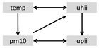Gangdong, Jungrang, Songpa, Yongsan
Type 3		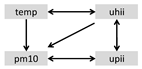Dongdaemun, Gangbuk, Jung, Seongbuk
Type 4		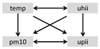Gangnam, Gwangjun, Seongdong
Type 5		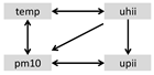Dobong, Gangseo
Type 6		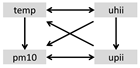Seocho, Seodaemun
Type 7		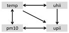Dongjak
Type 8		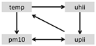Eunpyeong
Type 9		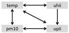Guro
Type 10		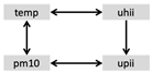Gwanak
Type 11		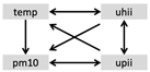Jongro
Type 12		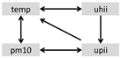Nowon

summarizes twelve distinct Granger-causal relationships.

Type 1 comprises the districts of Geumcheon, Mapo, Yangcheon, and Yeongdeungpo, each exhibiting the following characteristics: (1) daily average temperature Granger-causes UHII, daily average PM₁₀ concentration, and UPII; (2) UHII Granger-causes daily average temperature, daily average PM₁₀ concentration, and UPII; (3) daily average PM₁₀ concentration Granger-causes UPII; and (4) UPII Granger-causes daily average temperature and daily average PM₁₀ concentration. Type 2 includes Gangdong, Jungrang, Songpa, and Yongsan districts and yields the following causalities: (1) daily average temperature Granger-causes UHII and daily average PM₁₀ concentration; (2) UHII Granger-causes daily average temperature and UPII; (3) daily average PM₁₀ concentration Granger-causes UPII; and (4) UPII Granger-causes daily average PM₁₀ concentration. Dongdaemun, Gangbuk, Jung, and Seongbuk districts constitute Type 3, displaying the following relationships: (1) daily average temperature Granger-causes UHII and daily average PM₁₀ concentration; (2) UHII Granger-causes daily average temperature, daily average PM₁₀ concentration, and UPII; (3) daily average PM₁₀ concentration Granger-causes UPII; and (4) UPII Granger-causes daily average PM₁₀ concentration and UHII. Type 4 is represented by the districts of Gangnam, Gwangjin, and Seongdong, all of which share the following: (1) daily average temperature Granger-causes UHII, daily average PM₁₀ concentration, and UPII; (2) UHII Granger-causes daily average temperature, daily average PM₁₀ concentration, and UPII; (3) daily average PM₁₀ concentration Granger-causes UPII; and (4) UPII Granger-causes daily average PM₁₀ concentration.

Type 5 is composed of Dobong and Gangseo districts, which present the following: (1) daily average temperature Granger-causes UHII and daily average PM₁₀ concentration; (2) UHII Granger-causes daily average temperature, daily average PM₁₀ concentration, and UPII; (3) daily average PM₁₀ concentration Granger-causes daily average temperature and UPII; and (4) UPII Granger-causes daily average PM₁₀ concentration. Type 6 consists of Seocho and Seodaemun districts, which share the following: (1) daily average temperature Granger-causes UHII and daily average PM₁₀ concentration; (2) UHII Granger-causes daily average temperature, daily average PM₁₀ concentration, and UPII; (3) daily average PM₁₀ concentration Granger-causes UPII; and (4) UPII Granger-causes daily average temperature and daily average PM₁₀ concentration. Types 7 through 12 are represented by the districts of Dongjak, Eunpyeong, Guro, Gwanak, Jongro, and Nowon, respectively. Like the previous six, they also yield distinctive mixes of Granger causality pairs.

3.4. IRFs and FEVD Results

Table 5. Exemplary IRFs for twelve pairs of impulse and response variables.

Impulse Variable	Response Variable	Exemplary IRFs
temp	uhii	Gangdong
	pm10	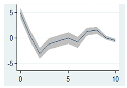Gwanak	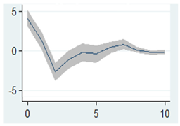Songpa
	upii	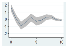Gangnam	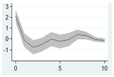Guro	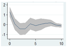Geumcheon
uhii	temp	Gangdong	Nowon
	pm10	Gangdong	Seodaemun
	upii	Gangdong	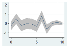Seodaemun	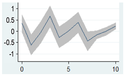Nowon
pm10	temp	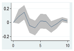Gwanak	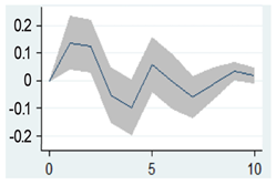Nowon
	upii	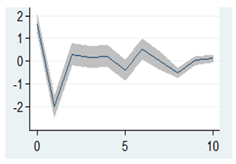Gangdong
upii	pm10	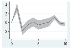Gangdong
	temp	Seodaemun	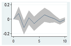Nowon
	uhii	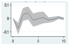Gangbuk	Jongro

Note: no IRFs are generated in cases where the impulse variable is pm10 and the response variable is uhii due to the absence of identified Granger causalities.

displays IRFs for the Granger-causal relationships within this analysis. It highlights a selected subset of exemplary functions, each exemplifying distinctive patterns, from a total of 400 functions, with 16 functions dedicated to each district. Notably, the table excludes the scenario in which the impulse variable is pm10 and the response variable is uhii, as no causal relationship was identified in that case.

To elaborate on a few, firstly, when the impulse variable is temp and the response variable is uhii, as shown in the first row of the table, the effect of a one-standard-deviation shock in daily average temperature becomes apparent. Initially, UHII exhibits a positive response, starting at 0 in period 1. A subsequent negative reaction occurs between periods 3 and 4, followed by a gradual convergence toward 0. Predominantly positive trends persist until later periods, with a significant positive reaction around the sixth or seventh period. However, despite this, the impact diminishes after 4 days, as indicated by the confidence interval encompassing 0. This pattern in Gangdong district aligns with similar trends observed in other districts. Second, when the impulse variable is uhii and the response variable is upii, the effect of a one-standard-deviation shock in UHII yields impacts on UPUII in three distinctive patterns. In the Gangdong case, an initial positive response in the first period was swiftly countered by a negative reaction in the second period. Stability marked periods 3 to 5, with short fluctuations in periods 6 and 7. Other periods showed no notable response. Seodaemun exhibited a similar but less significant pattern up to the fifth period, with significant reactions in the sixth and seventh stages. Nowon displayed an initial positive response, followed by alternating negative and positive reactions. Statistically significant responses were observed in the first, third, and seventh stages, with no substantial reactions in other periods.

Overall, the analysis revealed that all the IRFs exhibited immediate shocks in the early stages, typically up to the seventh period, but then gradually converged to 0 or reached statistically insignificant levels of response.

As indicated in

Table 6. Summary of FEVD results.

Impulse Variable	Response Variable
	temp	uhii	pm10	upii
temp	93.79%~97.73%	14.08%~40.04%	3.66%~8.16%	1.02%~4.89%
uhii	0.68%~5.24%	58.96%~85.12%	0.35%~1.46%	0.78%~2.48%
pm10	0.35%~1.11%	0.23%~1.16%	86.05%~92.68%	5.90%~26.17%
upii	0.30%~1.15%	0.07%~1.11%	1.84%~5.16%	67.45%~87.95%

, which presents the FEVD results for all relationships, during the 10th period, a significant portion of the variance in each of the four variables can be attributed to their own past values. Notably, daily average temperature demonstrates the highest degree of self-explanation, ranging from 93.79% to 97.73%. Following closely is daily average PM₁₀ concentration, accounting for 86.05% to 92.68% of its own variance. UPII explains 67.45% to 87.95% of its variance, while UHII shows the lowest self-explanation, ranging from 58.96% to 85.12%. This suggests that the two intensity variables, UHII and UPII, are relatively more influenced by their own past values than by other variables. UHII and UPII are also somewhat affected by daily average temperature and daily average PM₁₀ concentration, respectively. For a more compact presentation, the FEVD results for each district by each causal relationship are presented in Appendix B.

4. Discussion

What has been presented thus far warrants in-depth discussion. First, in terms of the thermal environment, our analysis has revealed a bidirectional Granger causality between daily average temperature and UHII in most cases. The IRFs showed that, with the exception of the Nowon district, a substantial positive response was exhibited when subjected to shocks in daily average temperature and UHII. The FEVD results emphasize that beyond their inherent influence, daily average temperature was significantly influenced by UHII, and UHII was predominantly shaped by daily average temperature across all districts. Second, concerning the air pollution variables, daily average PM₁₀ concentration and UPII, Granger causality was observed in both directions throughout Seoul, with an initial positive response in each case. Third, in districts categorized as types 1 and 2, our analysis indicates that the thermal environment Granger-caused air pollution in one direction. The IRFs revealed that the air pollution variables initially exhibited a notable positive response to shocks in the thermal environment, signifying the rapid deterioration of air pollution due to changes in the thermal environment. The FEVD results indicate that the overall influence of temperature on air pollution variables exceeded that of UHII. Fourth, in the majority of districts in Seoul, specifically types 3 to 12, a complex interaction between the thermal environment and air pollution was observed. The IRF analysis reveals an initial positive response, indicating that air pollution worsens due to changes in the thermal environment and vice versa. However, the response of the thermal environment to UPII shocks generally displayed an initial negative reaction. The FEVD results indicate that, in general, the thermal environment has a greater influence on air pollution than the reverse.

Figure 6 presents a comprehensive summary. (1) Daily average temperature and UHII display two-way Granger-causal relationships in 24 districts, with only one district showing daily average temperature as the Granger cause of UHII. (2) Daily average PM₁₀ concentration and UPII reveal two-way Granger-causal relationships across all 25 districts. (3) Daily average temperature and daily average PM₁₀ concentration exhibit two-way Granger-causal relationships in 6 districts. Meanwhile, daily average temperature Granger-causes daily average PM₁₀ concentration in 19 districts. (4) UHII and UPII establish two-way Granger-causal relationships in 5 districts, with UHII acting as the Granger cause of UPII in 20 districts. (5) Daily average temperature and UPII demonstrate two-way Granger-causal relationships in five districts. In four districts, daily average temperature Granger-causes UPII, while UPII Granger-causes daily average temperature in five districts. (6) Daily average PM₁₀ concentration and UHII do not exhibit any two-way Granger-causal relationships. However, daily average PM₁₀ concentration Granger-causes UHII in 4 districts, while UHII Granger-causes daily average PM₁₀ concentration in 16 districts.

Our findings are generally in line with what previous studies set forth. The one-way causal relationships, where either thermal environment is the independent variable and air pollution is the dependent [21,22,23,24,25,26,27,28,29,30] or the other way around [31,32,33,34], are evident in all districts of Seoul. At the same time, each district yields at least one two-way causal relationship, as another body of literature suggests [35,36,37,38,39,40].

Our contribution lies in moving beyond surface-level observations. Unlike prior studies, we reveal the coexistence of both one-way and two-way causal relationships within Seoul. Furthermore, our findings highlight the complexity of these relationships across the city’s 25 districts, indicating diverse combinations of causal interactions. This nuanced understanding underscores the variability of causal relationships within a city.

5. Conclusions

This study investigated the relationship between the thermal environment and air pollution in Seoul’s 25 districts, conducting a VAR Granger causality test to figure out causal relationships and IRF and FEVD to discover dynamic relationships. Major findings of this study can be summarized as follows. There exists a bidirectional Granger causality relationship between two thermal environment variables, namely the daily average temperature and UHII, in nearly all districts examined. Similarly, a bidirectional relationship is evident between the two air pollution variables, daily average PM₁₀ concentration and UPII, across all 25 districts. Simultaneously, it is noteworthy that a greater number of districts in general exhibit a Granger causality relationship from thermal environment variables to air pollution variables.

The conclusion of this study yields several policy recommendations. First is the concurrent management of temperature and UHIs. Our findings support the idea of simultaneously addressing temperature and UHII. While many climate action plans focus on reducing temperature through various adaptation strategies, they often overlook temperature variations across urban regions. Second, the simultaneous management of PM₁₀ concentration and UPII is crucial. Current air pollution policies have primarily concentrated on reducing air pollutants, neglecting the concept of urban pollution islands. Therefore, alongside existing air quality improvement goals, it is imperative to establish air quality standards that account for differences in urban and suburban air quality levels. Third, especially in most districts where one-way Granger-causal relationships exist, with thermal environment variables influencing air pollution variables but not vice versa, more emphasis on the former is crucial. Lastly, this holistic approach to managing the thermal environment and air pollution should be guided by the region-wide real-time monitoring of temperature and air pollution levels so as to provide an evidence-based roadmap for policymakers.

This study acknowledges several limitations. First, although we have uncovered complex links between the thermal environment and air pollution in Seoul’s 25 districts, the use of a VAR Granger causality test fails to clearly present specific factors that contribute to the diverse causal relationships. Second, although we are using five years of time series data, results from the statistical models do not capture relationships that may change over time. Third, the study’s reliance on pre-COVID-19 data means that it does not account for potential shifts in these relationships post-COVID-19. Lastly, our data are confined within the spatial boundaries of Seoul and exploring data beyond the city may yield varied results, potentially leading to different insights and recommendations.

Despite its limitations, this study represents one of the pioneering endeavors to comprehensively unveil the intricate interplay between the thermal environment and air pollution. The insights derived from Seoul have the potential to significantly aid other regions worldwide that are grappling with comparable environmental issues. These findings can serve as valuable guidance for communities striving to create healthier and more sustainable urban environments globally.

References

- Son, G.; Hwang, W. Consumers’ Views on ESG and Environmental Friendly Consumption Behavior; KB Financial Group: Seoul, Republic of Korea, 2021. [Google Scholar]
- Hwang, I.; Baek, J. Market Mechanisms for Addressing Climate Change and Air Pollution in Seoul; Seoul Institute: Seoul, Republic of Korea, 2020. [Google Scholar]
- Korea Meteorological Administration. Korean Climate Change Assessment Report 2020: Scientific Basis for Climate Change (Summary for Policymakers); Korea Meteorological Administration: Seoul, Republic of Korea, 2020.
- OECD. How’s Life? 2020: Measuring Well-Being. Available online: https://www.oecd.org/wise/how-s-life-23089679.htm (accessed on 22 August 2023).
- Kim, H. Seasonal Impacts of Particulate Matter Levels on Bike Sharing in Seoul, South Korea. Int. J. Environ. Res. Public Health 2020, 17, 3999. [Google Scholar] [CrossRef] [PubMed]
- Kim, H. Land Use Impacts on Particulate Matter Levels in Seoul, South Korea: Comparing High and Low Seasons. Land 2020, 9, 142. [Google Scholar] [CrossRef]
- Shin, J.; Yang, H.; Kim, C. The Relationship between Climate and Energy Consumption: The Case of South Korea. Energy Sources Part A Recovery Util. Environ. Eff. 2023, 45, 6456–6471. [Google Scholar] [CrossRef]
- Lee, K.; Baek, H.-J.; Cho, C. The Estimation of Base Temperature for Heating and Cooling Degree-Days for South Korea. J. Appl. Meteorol. Climatol. 2014, 53, 300–309. [Google Scholar] [CrossRef]
- Lim, Y.-H.; Lee, K.-S.; Bae, H.-J.; Kim, D.; Yoo, H.; Park, S.; Hong, Y.-C. Estimation of Heat-Related Deaths during Heat Wave Episodes in South Korea (2006–2017). Int. J. Biometeorol. 2019, 63, 1621–1629. [Google Scholar] [CrossRef] [PubMed]
- Park, J.; Chae, Y.; Choi, S.H. Analysis of Mortality Change Rate from Temperature in Summer by Age, Occupation, Household Type, and Chronic Diseases in 229 Korean Municipalities from 2007–2016. Int. J. Environ. Res. Public Health 2019, 16, 1561. [Google Scholar] [CrossRef] [PubMed]
- Kim, J.; Song, K.J.; Hong, K.J.; Ro, Y.S. Trend of Outbreak of Thermal Illness Patients Based on Temperature 2002–2013 in Korea. Climate 2017, 5, 94. [Google Scholar] [CrossRef]
- Kim, O.-J.; Lee, S.H.; Kang, S.-H.; Kim, S.-Y. Incident Cardiovascular Disease and Particulate Matter Air Pollution in South Korea Using a Population-Based and Nationwide Cohort of 0.2 Million Adults. Environ. Health 2020, 19, 113. [Google Scholar] [CrossRef]
- Kim, J.-H.; Oh, I.-H.; Park, J.-H.; Cheong, H.-K. Premature Deaths Attributable to Long-Term Exposure to Ambient Fine Particulate Matter in the Republic of Korea. J. Korean Med. Sci. 2018, 33, e251. [Google Scholar] [CrossRef]
- Wheeler, S.M. Planning for Sustainability: Creating Livable, Equitable and Ecological Communities; Routledge: New York, NY, USA, 2013; ISBN 978-0-415-80989-4. [Google Scholar]
- Newman, P.; Beatley, T.; Boyer, H. Resilient Cities: Responding to Peak Oil and Climate Change; Island Press: Washington, DC, USA, 2009; ISBN 978-1-59726-498-3. [Google Scholar]
- Newman, P.; Kenworthy, J. Sustainability and Cities: Overcoming Automobile Dependence; Island Press: Washington, DC, USA, 1999; ISBN 978-1-55963-660-5. [Google Scholar]
- Calthorpe, P. Urbanism in the Age of Climate Change, 2nd ed.; Island Press: Washington, DC, USA, 2013; ISBN 978-1-59726-721-2. [Google Scholar]
- Moussiopoulos, N. Air Quality in Cities; Springer: Berlin/Heidelberg, Germany, 2003; ISBN 978-3-642-05646-8. [Google Scholar]
- Zhang, D.; Zhou, C.; He, B.-J. Spatial and Temporal Heterogeneity of Urban Land Area and PM2.5 Concentration in China. Urban Clim. 2022, 45, 101268. [Google Scholar] [CrossRef]
- Ross, Z.; Jerrett, M.; Ito, K.; Tempalski, B.; Thurston, G.D. A Land Use Regression for Predicting Fine Particulate Matter Concentrations in the New York City Region. Atmos. Environ. 2007, 41, 2255–2269. [Google Scholar] [CrossRef]
- Stafoggia, M.; Bellander, T.; Bucci, S.; Davoli, M.; de Hoogh, K.; de’ Donato, F.; Gariazzo, C.; Lyapustin, A.; Michelozzi, P.; Renzi, M.; et al. Estimation of Daily PM10 and PM2.5 Concentrations in Italy, 2013–2015, Using a Spatiotemporal Land-Use Random-Forest Model. Environ. Int. 2019, 124, 170–179. [Google Scholar] [CrossRef] [PubMed]
- Zhang, Z.; Wang, J.; Hart, J.E.; Laden, F.; Zhao, C.; Li, T.; Zheng, P.; Li, D.; Ye, Z.; Chen, K. National Scale Spatiotemporal Land-Use Regression Model for PM2.5, PM10 and NO2 Concentration in China. Atmos. Environ. 2018, 192, 48–54. [Google Scholar] [CrossRef]
- Kim, H.; Hong, S. Relationship between Land-Use Type and Daily Concentration and Variability of PM10 in Metropolitan Cities: Evidence from South Korea. Land 2022, 11, 23. [Google Scholar] [CrossRef]
- Ahn, H.; Lee, J.; Hong, A. Urban Form and Air Pollution: Clustering Patterns of Urban Form Factors Related to Particulate Matter in Seoul, Korea. Sustain. Cities Soc. 2022, 81, 103859. [Google Scholar] [CrossRef]
- Park, Y.; Shin, J.; Lee, J.Y. Spatial Association of Urban Form and Particulate Matter. Int. J. Environ. Res. Public Health 2021, 18, 9428. [Google Scholar] [CrossRef]
- McCarty, J.; Kaza, N. Urban Form and Air Quality in the United States. Landsc. Urban Plan. 2015, 139, 168–179. [Google Scholar] [CrossRef]
- Sarrat, C.; Lemonsu, A.; Masson, V.; Guedalia, D. Impact of Urban Heat Island on Regional Atmospheric Pollution. Atmos. Environ. 2006, 40, 1743–1758. [Google Scholar] [CrossRef]
- Akbari, H.; Pomerantz, M.; Taha, H. Cool Surfaces and Shade Trees to Reduce Energy Use and Improve Air Quality in Urban Areas. Sol. Energy 2001, 70, 295–310. [Google Scholar] [CrossRef]
- Akbari, H. Shade Trees Reduce Building Energy Use and CO2 Emissions from Power Plants. Environ. Pollut. 2002, 116, S119–S126. [Google Scholar] [CrossRef]
- Stone, B. Urban Heat and Air Pollution: An Emerging Role for Planners in the Climate Change Debate. J. Am. Plan. Assoc. 2005, 71, 13–25. [Google Scholar] [CrossRef]
- Jin, M.; Shepherd, J.M.; Zheng, W. Urban Surface Temperature Reduction via the Urban Aerosol Direct Effect: A Remote Sensing and WRF Model Sensitivity Study. Adv. Meteorol. 2011, 2010, e681587. [Google Scholar] [CrossRef]
- Jin, M.S.; Kessomkiat, W.; Pereira, G. Satellite-Observed Urbanization Characters in Shanghai, China: Aerosols, Urban Heat Island Effect, and Land–Atmosphere Interactions. Remote Sens. 2011, 3, 83–99. [Google Scholar] [CrossRef]
- Li, H.; Sodoudi, S.; Liu, J.; Tao, W. Temporal Variation of Urban Aerosol Pollution Island and Its Relationship with Urban Heat Island. Atmos. Res. 2020, 241, 104957. [Google Scholar] [CrossRef]
- Cao, C.; Lee, X.; Liu, S.; Schultz, N.; Xiao, W.; Zhang, M.; Zhao, L. Urban Heat Islands in China Enhanced by Haze Pollution. Nat. Commun. 2016, 7, 12509. [Google Scholar] [CrossRef] [PubMed]
- Ngarambe, J.; Joen, S.J.; Han, C.-H.; Yun, G.Y. Exploring the Relationship between Particulate Matter, CO, SO2, NO2, O3 and Urban Heat Island in Seoul, Korea. J. Hazard. Mater. 2021, 403, 123615. [Google Scholar] [CrossRef] [PubMed]
- Lai, L.-W.; Cheng, W.-L. Air Quality Influenced by Urban Heat Island Coupled with Synoptic Weather Patterns. Sci. Total Environ. 2009, 407, 2724–2733. [Google Scholar] [CrossRef]
- Xu, L.Y.; Xie, X.D.; Li, S. Correlation Analysis of the Urban Heat Island Effect and the Spatial and Temporal Distribution of Atmospheric Particulates Using TM Images in Beijing. Environ. Pollut. 2013, 178, 102–114. [Google Scholar] [CrossRef]
- Li, H.; Meier, F.; Lee, X.; Chakraborty, T.; Liu, J.; Schaap, M.; Sodoudi, S. Interaction between Urban Heat Island and Urban Pollution Island during Summer in Berlin. Sci. Total Environ. 2018, 636, 818–828. [Google Scholar] [CrossRef]
- Zheng, Z.; Ren, G.; Wang, H.; Dou, J.; Gao, Z.; Duan, C.; Li, Y.; Ngarukiyimana, J.P.; Zhao, C.; Cao, C.; et al. Relationship Between Fine-Particle Pollution and the Urban Heat Island in Beijing, China: Observational Evidence. Bound.-Layer Meteorol. 2018, 169, 93–113. [Google Scholar] [CrossRef]
- Sabrin, S.; Karimi, M.; Nazari, R. Developing Vulnerability Index to Quantify Urban Heat Islands Effects Coupled with Air Pollution: A Case Study of Camden, NJ. ISPRS Int. J. Geo-Inf. 2020, 9, 349. [Google Scholar] [CrossRef]
- Ulpiani, G. On the Linkage between Urban Heat Island and Urban Pollution Island: Three-Decade Literature Review towards a Conceptual Framework. Sci. Total Environ. 2021, 751, 141727. [Google Scholar] [CrossRef] [PubMed]
- Lindsey, R.; Dahlman, L. Climate Change: Global Temperature. Available online: http://www.climate.gov/news-features/understanding-climate/climate-change-global-temperature (accessed on 23 August 2023).
- Han, B.-S.; Park, K.; Kwak, K.-H.; Park, S.-B.; Jin, H.-G.; Moon, S.; Kim, J.-W.; Baik, J.-J. Air Quality Change in Seoul, South Korea under COVID-19 Social Distancing: Focusing on PM2.5. Int. J. Environ. Res. Public Health 2020, 17, 6208. [Google Scholar] [CrossRef] [PubMed]
- Kim, S.-U.; Kim, K.-Y. Physical and Chemical Mechanisms of the Daily-to-Seasonal Variation of PM10 in Korea. Sci. Total Environ. 2020, 712, 136429. [Google Scholar] [CrossRef] [PubMed]
- Oke, T.R. Boundary Layer Climates; Routledge: New York, NY, USA, 1987; ISBN 978-0-415-04319-9. [Google Scholar]
- Oke, T.R. The Distinction between Canopy and Boundary-layer Urban Heat Islands. Atmosphere 1976, 14, 268–277. [Google Scholar] [CrossRef]
- Crutzen, P.J. New Directions: The Growing Urban Heat and Pollution “Island” Effect—Impact on Chemistry and Climate. Atmos. Environ. 2004, 38, 3539–3540. [Google Scholar] [CrossRef]
- Zhou, B.; Rybski, D.; Kropp, J.P. On the Statistics of Urban Heat Island Intensity. Geophys. Res. Lett. 2013, 40, 5486–5491. [Google Scholar] [CrossRef]
- Li, Y.; Schubert, S.; Kropp, J.P.; Rybski, D. On the Influence of Density and Morphology on the Urban Heat Island Intensity. Nat. Commun. 2020, 11, 2647. [Google Scholar] [CrossRef]
- Dewan, A.; Kiselev, G.; Botje, D.; Mahmud, G.I.; Bhuian, H.; Hassan, Q.K. Surface Urban Heat Island Intensity in Five Major Cities of Bangladesh: Patterns, Drivers and Trends. Sustain. Cities Soc. 2021, 71, 102926. [Google Scholar] [CrossRef]
- Kim, Y.-H.; Baik, J.-J. Maximum Urban Heat Island Intensity in Seoul. J. Appl. Meteorol. Climatol. 2002, 41, 651–659. [Google Scholar] [CrossRef]
- Park, J.; Kim, J.-H.; Sohn, W.; Lee, D.-K. Urban Cooling Factors: Do Small Greenspaces Outperform Building Shade in Mitigating Urban Heat Island Intensity? Urban For. Urban Green. 2021, 64, 127256. [Google Scholar] [CrossRef]
- Jeong, S.-J.; Park, H.; Ho, C.-H.; Kim, J. Impact of Urbanization on Spring and Autumn Phenology of Deciduous Trees in the Seoul Capital Area, South Korea. Int. J. Biometeorol. 2019, 63, 627–637. [Google Scholar] [CrossRef] [PubMed]
- Sims, C.A. Macroeconomics and Reality. Econometrica 1980, 48, 1–48. [Google Scholar] [CrossRef]
- Wang, N.; Guo, J.; Liu, X.; Fang, T. A Service Demand Forecasting Model for One-Way Electric Car-Sharing Systems Combining Long Short-Term Memory Networks with Granger Causality Test. J. Clean. Prod. 2020, 244, 118812. [Google Scholar] [CrossRef]
- Zhao, K.; Chen, D.; Zhang, X.; Zhang, X. How Do Urban Land Expansion, Land Finance, and Economic Growth Interact? Int. J. Environ. Res. Public Health 2022, 19, 5039. [Google Scholar] [CrossRef] [PubMed]
- Sunde, T. Energy Consumption and Economic Growth Modelling in SADC Countries: An Application of the VAR Granger Causality Analysis. Int. J. Energy Technol. Policy 2020, 16, 41–56. [Google Scholar] [CrossRef]
- Dickey, D.A.; Fuller, W.A. Distribution of the Estimators for Autoregressive Time Series with a Unit Root. J. Am. Stat. Assoc. 1979, 74, 427–431. [Google Scholar] [CrossRef]
- Granger, C.W.J. Investigating Causal Relations by Econometric Models and Cross-Spectral Methods. Econometrica 1969, 37, 424–438. [Google Scholar] [CrossRef]
- Liu, H.; Kim, H. Ecological Footprint, Foreign Direct Investment, and Gross Domestic Production: Evidence of Belt & Road Initiative Countries. Sustainability 2018, 10, 3527. [Google Scholar] [CrossRef]
- Pereira, A.M.; de Frutos, R.F. Public Capital Accumulation and Private Sector Performance. J. Urban Econ. 1999, 46, 300–322. [Google Scholar] [CrossRef]
- Chaiechi, T.; Nguyen, T.M.T. Measuring Urban Economic Resilience of Two Tropical Cities, Using Impulse Response Analysis. Bull. Appl. Econ. 2021, 8, 59–79. [Google Scholar] [CrossRef]
- Bildirici, M.; Ozaksoy, F. The Relationship between Woody Biomass Consumption and Economic Growth: Nonlinear ARDL and Causality. J. For. Econ. 2017, 27, 60–69. [Google Scholar] [CrossRef]
- Liao, W.-C.; Zhao, D.; Lim, L.P.; Wong, G.K.M. Foreign Liquidity to Real Estate Market: Ripple Effect and Housing Price Dynamics. Urban Stud. 2015, 52, 138–158. [Google Scholar] [CrossRef]