
Identifying Impacts of School-Escorted Trips on Traffic Congestion and the Countermeasures in Bangkok: An Agent-Based Simulation Approach

Abstract
:1. Introduction
2. Literature Review
2.1. School Trips on Urban Congestion and Pollution
2.2. Agent-Based Model
2.3. Time Shift Scenario
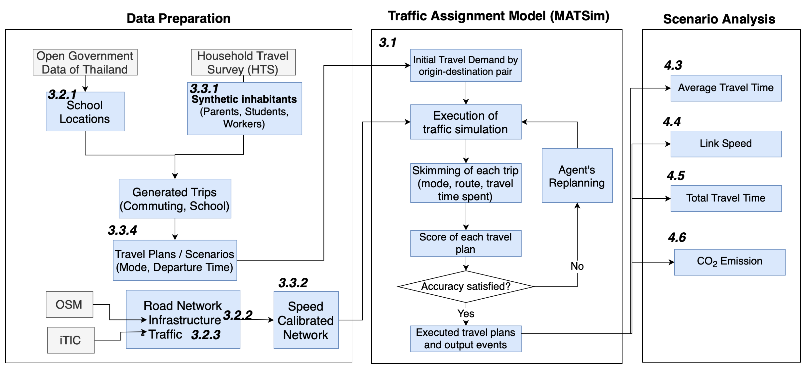
3. Methodology and Data
3.1. Methodology
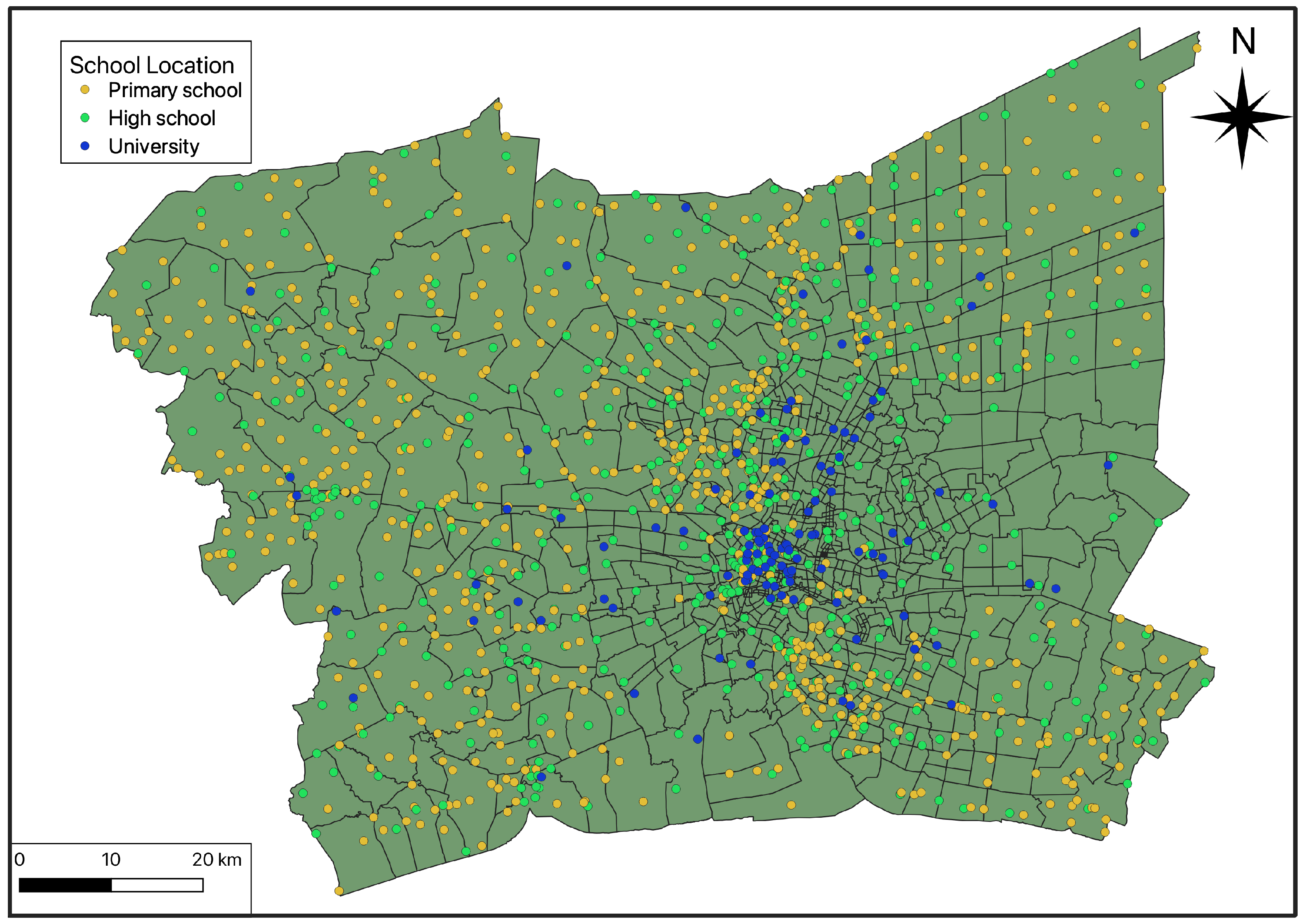
3.2. Spatial Data
3.2.1. School Locations
3.2.2. Road Network
3.2.3. Traffic Data
3.3. Preparation for MATSim Simulation
3.3.1. Generating Agents
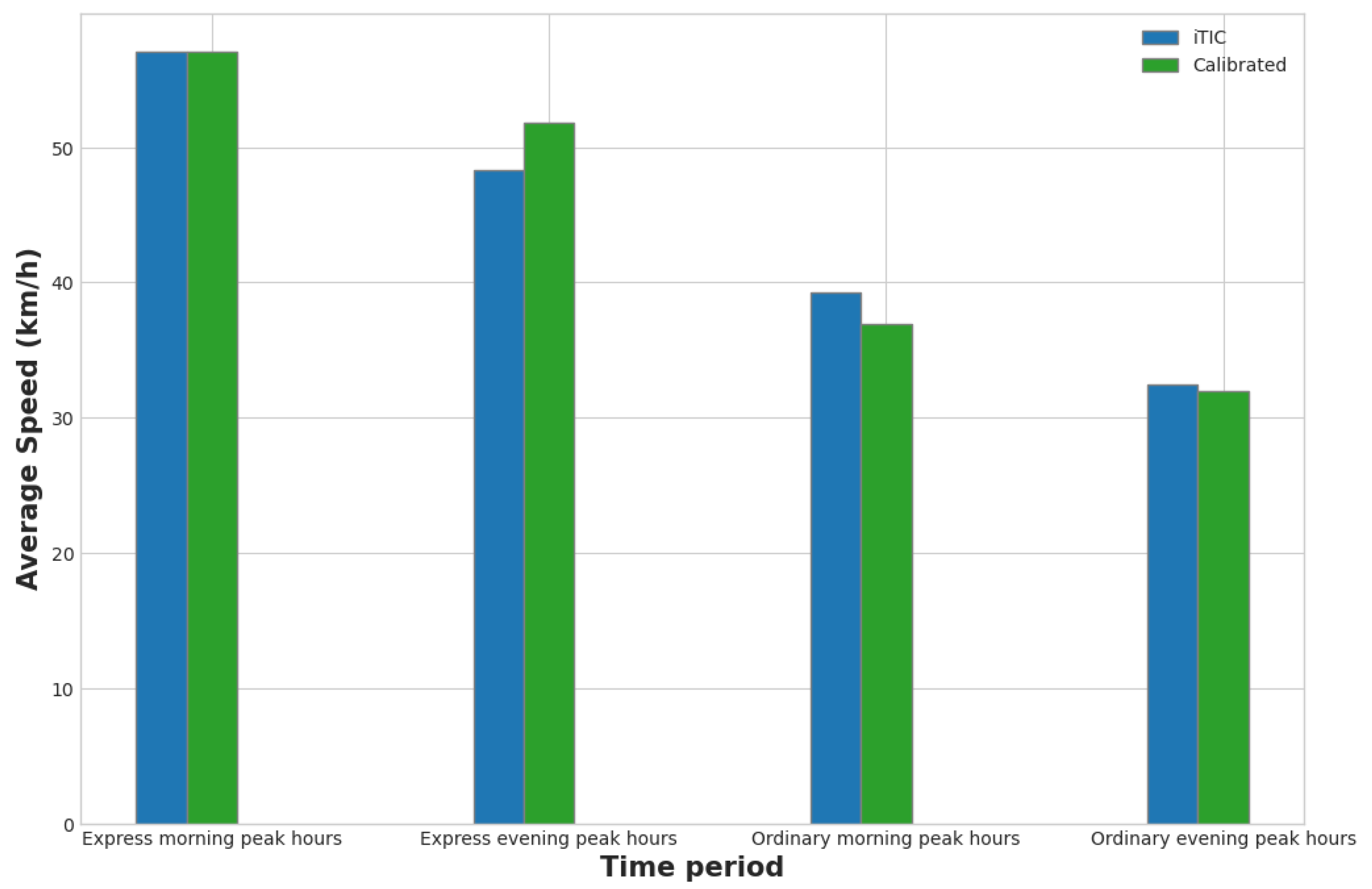
3.3.2. Network Calibration
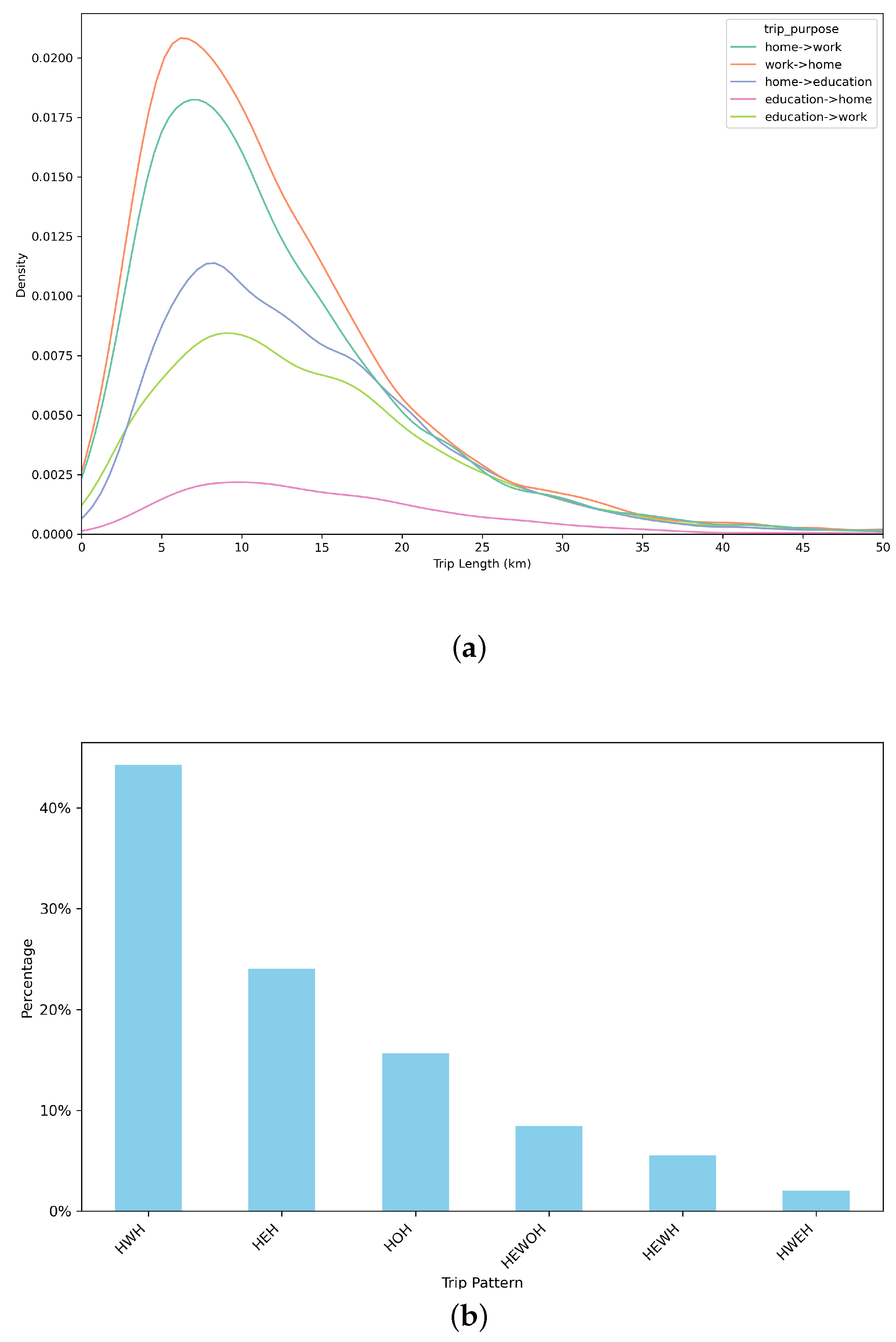
3.3.3. Model Validation
4. Comparison of Alternative Scenarios
4.1. Setting Up Scenarios
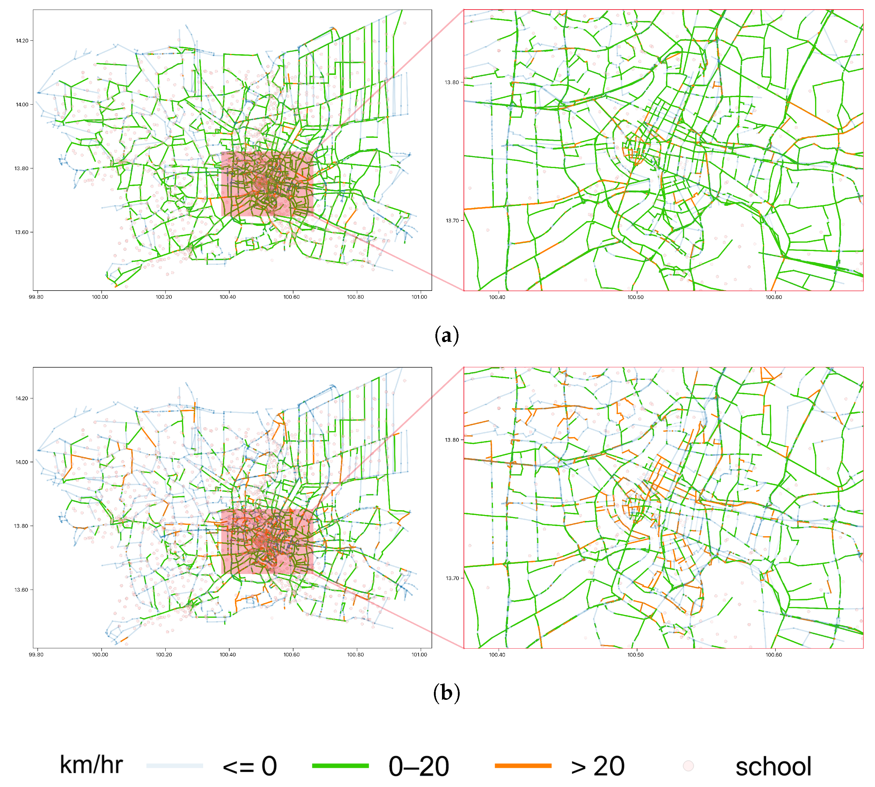
4.2. Effects of School Trip Reduction on Urban Traffic Congestion
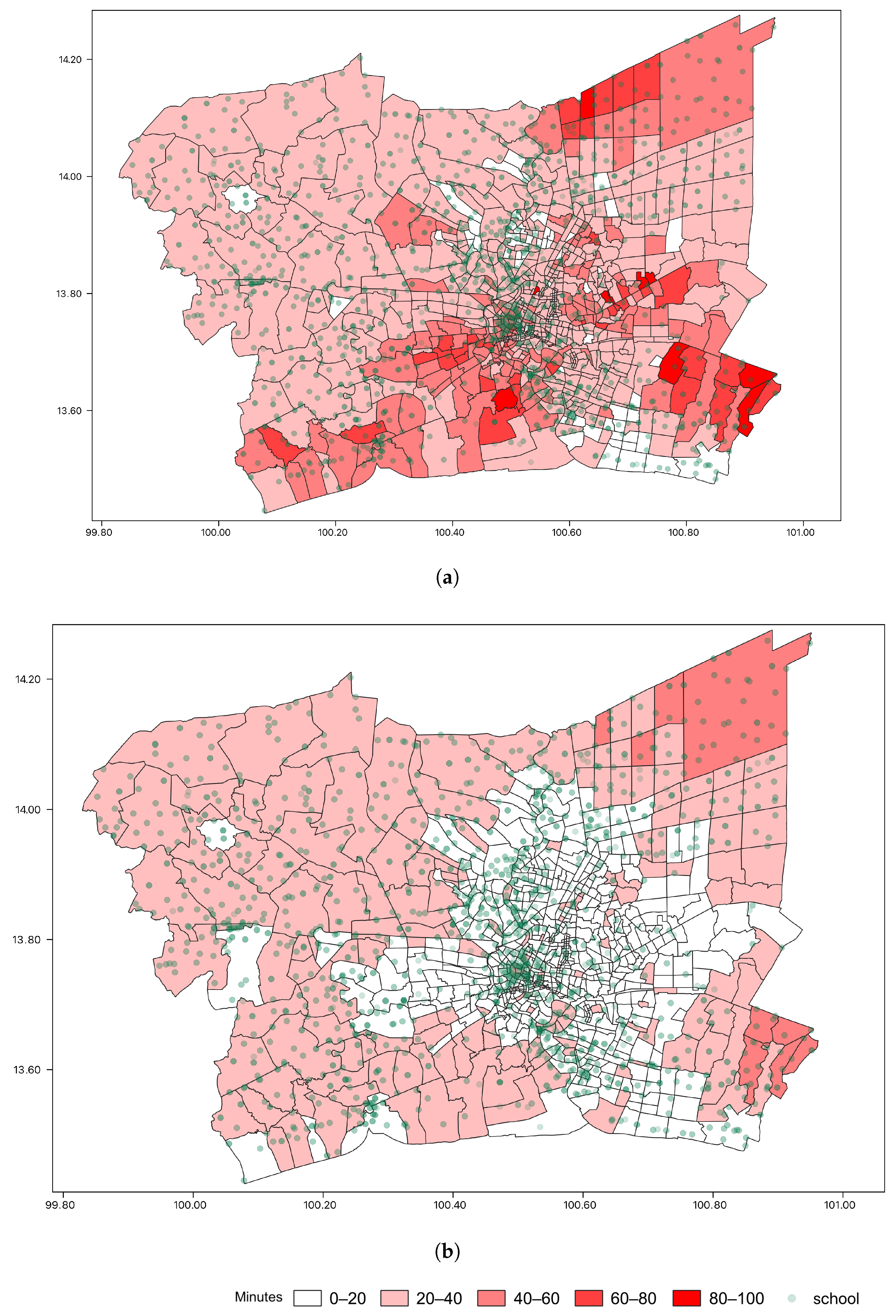
4.3. Average Travel Time per Trip among TAZs
4.4. Comparison of Average Speed over All Links between Scenarios
4.5. Total Travel Time
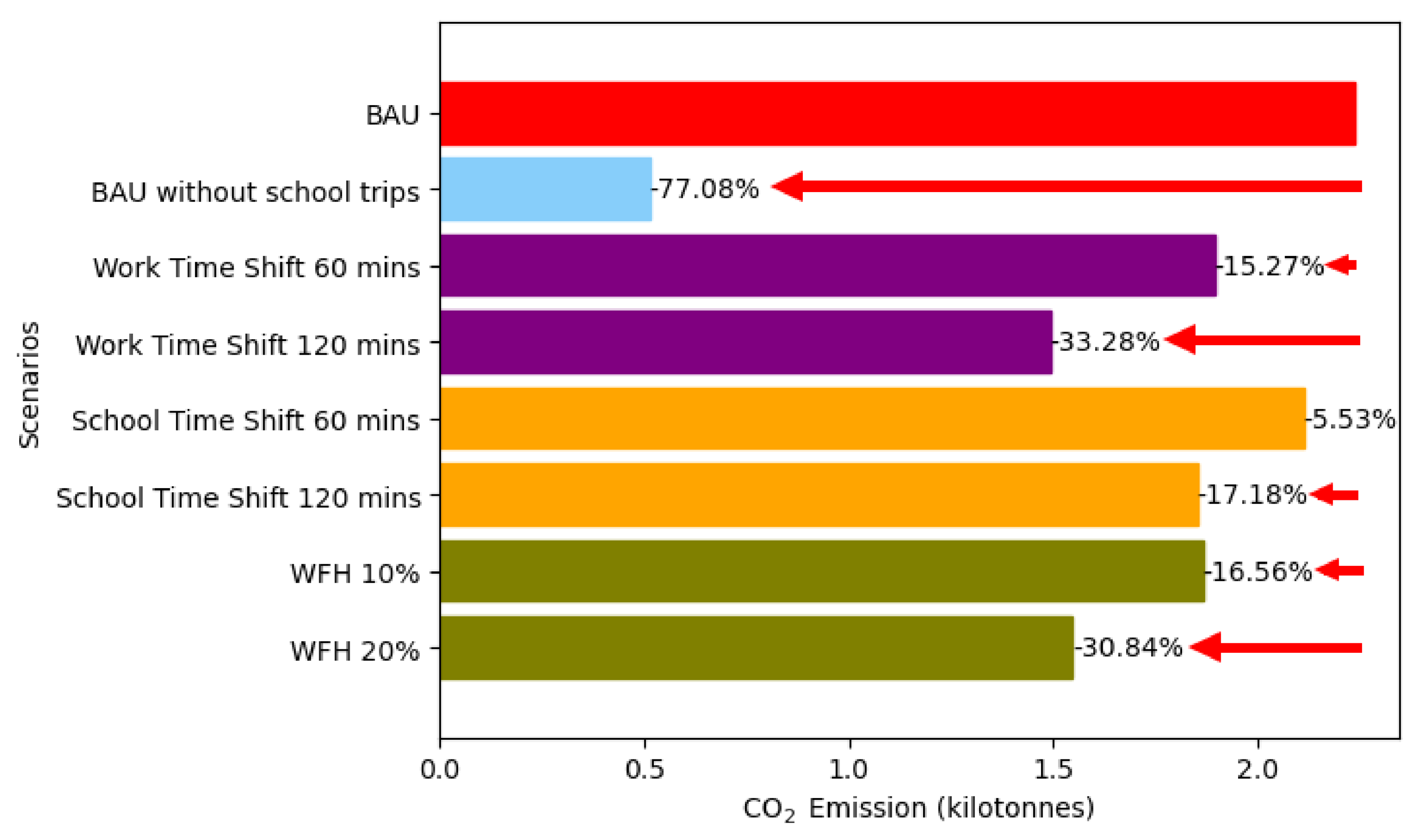
4.6. CO2 Emission
5. Conclusions
5.1. Effects of Alternative Scenarios
5.1.1. Flexible Working Time (Time Design, Scenario 3 and 4)
5.1.2. Staggered School Start Times (Time Design, Scenario 5 and 6)
5.1.3. Work from Home (Physical Urban Design, Scenario 7 and 8)
5.1.4. Local Physical Design
5.2. Policy Implication
5.3. Study Limitation and Future Research
Author Contributions
Funding
Institutional Review Board Statement
Informed Consent Statement
Data Availability Statement
Conflicts of Interest
Abbreviations
| MATSim | Multi-Agent Transport Simulation |
| TAZ | Traffic Analysis Zone |
| BAU | Business As Usual |
| HTS | Household Travel survey |
| iTIC | Intelligent Traffic Information Center |
| BMR | Bangkok Metropolitan Region |
References
- Vongpuapan, S.; Latchford, J. Traffic Management in Bangkok. In Proceedings of the Transportation Research Record, Washington, DC, USA, 14–17 January 1985. [Google Scholar]
- Vichiensan, V.; Wasuntarasook, V.; Hayashi, Y.; Kii, M.; Prakayaphun, T. Urban Rail Transit in Bangkok: Chronological Development Review and Impact on Residential Property Value. Sustainability 2022, 14, 284. [Google Scholar] [CrossRef]
- Ayaragarnchanakul, E.; Creutzig, F. Bangkok’s locked-in traffic jam: Price congestion or regulate parking? Case Stud. Transp. Policy 2022, 10, 365–378. [Google Scholar] [CrossRef]
- Lu, M.; Sun, C.; Zheng, S. Congestion and pollution consequences of driving-to-school trips: A case study in Beijing. Transp. Res. Part D Transp. Environ. 2017, 50, 280–291. [Google Scholar] [CrossRef]
- Rothman, L.; Buliung, R.; Howard, A.; Macarthur, C.; Macpherson, A. The school environment and student car drop-off at elementary schools. Travel Behav. Soc. 2017, 9, 50–57. [Google Scholar] [CrossRef]
- McMillan, T.E. The relative influence of urban form on a child’s travel mode to school. Transp. Res. Part A Policy Pract. 2007, 41, 69–79. [Google Scholar] [CrossRef]
- Curtis, C.; Babb, C.; Olaru, D. Built environment and children’s travel to school. Transp. Policy 2015, 42, 21–33. [Google Scholar] [CrossRef]
- Yeung, J.; Wearing, S.; Hills, A. Child transport practices and perceived barriers in active commuting to school. Transp. Res. Part A Policy Pract. 2008, 42, 895–900. [Google Scholar] [CrossRef]
- Zhang, R.; Yao, E.; Liu, Z. School travel mode choice in Beijing, China. J. Transp. Geogr. 2017, 62, 98–110. [Google Scholar] [CrossRef]
- Rojas López, M.C.; Wong, Y.D. Process and determinants of mobility decisions—A holistic and dynamic travel behaviour framework. Travel Behav. Soc. 2019, 17, 120–129. [Google Scholar] [CrossRef]
- Wilensky, U.; Rand, W. An Introduction to Agent-Based Modeling: Modeling Natural, Social, and Engineered Complex Systems with NetLogo; The MIT Press: Cambridge, MA, USA, 2015. [Google Scholar]
- Chiou, Y.S.; Bayer, A.Y. Microscopic Modeling of Pedestrian Movement in a Shida Night Market Street Segment: Using Vision and Destination Attractiveness. Sustainability 2021, 13, 8015. [Google Scholar] [CrossRef]
- Borshchev, A. Multi-method modelling: AnyLogic. In Discrete-Event Simulation and System Dynamics for Management Decision Making; John Wiley & Sons, Ltd.: Hoboken, NJ, USA, 2014; pp. 248–279. [Google Scholar] [CrossRef]
- Horni, A.; Nagel, K.; Axhausen, K. (Eds.) Multi-Agent Transport Simulation MATSim; Ubiquity Press: London, UK, 2016; p. 618. [Google Scholar] [CrossRef]
- Smith, L.; Beckman, R.; Baggerly, K. TRANSIMS: Transportation Analysis and Simulation System; U.S. Department of Energy: Washington, DC, USA, 1995. [CrossRef]
- Bastarianto, F.; Hancock, T.; Choudhury, C.; Manley, E. Agent-based models in urban transportation: Review, challenges, and opportunities. Eur. Transp. Res. Rev. 2023, 15, 19. [Google Scholar] [CrossRef]
- McNally, M.G. The Four Step Model. In Handbook of Transport Modelling; Emerald Group Publishing Limited: Bingley, UK, 2007. [Google Scholar]
- Bonabeau, E. Agent-based modeling: Methods and techniques for simulating human systems. Proc. Natl. Acad. Sci. USA 2002, 99 (Suppl. S3), 7280–7287. [Google Scholar] [CrossRef] [PubMed]
- He, B.Y.; Zhou, J.; Ma, Z.; Wang, D.; Sha, D.; Lee, M.; Chow, J.Y.; Ozbay, K. A validated multi-agent simulation test bed to evaluate congestion pricing policies on population segments by time-of-day in New York City. Transp. Policy 2021, 101, 145–161. [Google Scholar] [CrossRef]
- Kii, M.; Goda, Y.; Vichiensan, V.; Miyazaki, H.; Moeckel, R. Assessment of Spatiotemporal Peak Shift of Intra-Urban Transportation Taking a Case in Bangkok, Thailand. Sustainability 2021, 13, 6777. [Google Scholar] [CrossRef]
- Hörl, S.; Ruch, C.; Becker, F.; Frazzoli, E.; Axhausen, K. Fleet operational policies for automated mobility: A simulation assessment for Zurich. Transp. Res. Part C Emerg. Technol. 2019, 102, 20–31. [Google Scholar] [CrossRef]
- Ciari, F.; Balac, M.; Axhausen, K. Modeling Carsharing with the Agent-Based Simulation MATSim: State of the Art, Applications, and Future Developments. Transp. Res. Rec. J. Transp. Res. Board 2016, 2564, 14–20. [Google Scholar] [CrossRef]
- Goodman, W.D. Transportation and Staggered Work Hours. Transp. Law J. 1972, 4, 157. [Google Scholar]
- D’Este, G. The effect of staggered working hours on commuter trip durations. Transp. Res. Part A Gen. 1985, 19, 109–117. [Google Scholar] [CrossRef]
- Yildirimoglu, M.; Ramezani, M.; Amirgholy, M. Staggered work schedules for congestion mitigation: A morning commute problem. Transp. Res. Part C Emerg. Technol. 2021, 132, 103391. [Google Scholar] [CrossRef]
- Charypar, D.; Nagel, K. Generating complete all-day activity plans with genetic algorithms. Transportation 2005, 32, 369–397. [Google Scholar] [CrossRef]
- Ben-Dor, G.; Ben-Elia, E.; Benenson, I. Population downscaling in multi-agent transportation simulations: A review and case study. Simul. Model. Pract. Theory 2021, 108, 102233. [Google Scholar] [CrossRef]
- Achariyaviriya, W.; Hayashi, Y.; Takeshita, H.; Kii, M.; Vichiensan, V.; Theeramunkong, T. Can Space–Time Shifting of Activities and Travels Mitigate Hyper-Congestion in an Emerging Megacity, Bangkok? Effects on Quality of Life and CO2 Emission. Sustainability 2021, 13, 6547. [Google Scholar] [CrossRef]
- Lomax, N.; Norman, P. Estimating Population Attribute Values in a Table: “Get Me Started in” Iterative Proportional Fitting. Prof. Geogr. 2016, 68, 451–461. [Google Scholar] [CrossRef]
- Office of Transport and Traffic Policy and Planning. Results of a Travel Demand Survey in BMR. Available online: https://otp.gdcatalog.go.th/dataset/otp_66_02 (accessed on 10 November 2023).
- Achariyaviriya, W.; Suttakul, P.; Fongsamootr, T.; Mona, Y.; Phuphisith, S.; Tippayawong, K.Y. The social cost of carbon of different automotive powertrains: A comparative case study of Thailand. Energy Rep. 2023, 9, 1144–1151. [Google Scholar] [CrossRef]
- Bangkok Post. City Hall Orders Staggered Hours in Fight against Smog. Available online: https://www.bangkokpost.com/business/1840579/city-hall-orders-staggered-hours-in-fight-against-smog (accessed on 10 November 2023).
- Thai PBS. Cabinet Approved 3 Forms of Government Service for New Normal. Available online: https://www.thaipbs.or.th/news/content/319628 (accessed on 10 November 2023).
- Vichiensan, V.; Wasuntarasook, V.; Prakayaphun, T.; Kii, M.; Hayashi, Y. Influence of Urban Railway Network Centrality on Residential Property Values in Bangkok. Sustainability 2023, 15, 16013. [Google Scholar] [CrossRef]
- Ramadan, O.E.; Sisiopiku, V.P. A Critical Review on Population Synthesis for Activity- and Agent-Based Transportation Models. In Transportation Systems Analysis and Assessment; Luca, S.D., Pace, R.D., Djordjevic, B., Eds.; IntechOpen: Rijeka, Croatia, 2019; Chapter 1. [Google Scholar] [CrossRef]
- Bassolas, A.; Ramasco, J.J.; Herranz, R.; Cantú-Ros, O.G. Mobile phone records to feed activity-based travel demand models: MATSim for studying a cordon toll policy in Barcelona. Transp. Res. Part A Policy Pract. 2019, 121, 56–74. [Google Scholar] [CrossRef]


| Modules | Parameters | Values |
|---|---|---|
| QSim | Flow capacity factor | 0.15 |
| Storage capacity factor | 0.15 | |
| Traffic dynamics | queue | |
| Strategy | Keep-last-selected probability | 0.95 |
| Re-route probability | 0.3 |
| From | To | Link Speed | Quantity |
|---|---|---|---|
| 1506 | 1507 | 47.3 | 1 |
| 3222 | 3223 | 30.88 | 2 |
| 3223 | 3222 | 10.2 | 3 |
| Hour | Std | Mean | Min | Max |
|---|---|---|---|---|
| 6 | 13.50 | 40.47 | 12 | 98 |
| 7 | 14.28 | 36.41 | 11 | 93 |
| 8 | 14.08 | 35.99 | 10 | 91 |
| 16 | 14.02 | 35.14 | 9 | 92 |
| 17 | 13.79 | 32.97 | 8 | 90 |
| 18 | 13.81 | 31.89 | 8 | 89 |
| Travel Statistics | Observation | Simulation | |
|---|---|---|---|
| Car | Motorcycle | Car | |
| Average trip length (km/trip) | 16 | 10 | 12.9 |
| Travel time (min) | 36 | 24 | 34.2 |
| Average Speed (km/h) | 26 | 25 | 30.4 |
Disclaimer/Publisher’s Note: The statements, opinions and data contained in all publications are solely those of the individual author(s) and contributor(s) and not of MDPI and/or the editor(s). MDPI and/or the editor(s) disclaim responsibility for any injury to people or property resulting from any ideas, methods, instructions or products referred to in the content. |
© 2023 by the authors. Licensee MDPI, Basel, Switzerland. This article is an open access article distributed under the terms and conditions of the Creative Commons Attribution (CC BY) license (https://creativecommons.org/licenses/by/4.0/).
Share and Cite
Prakayaphun, T.; Hayashi, Y.; Vichiensan, V.; Takeshita, H. Identifying Impacts of School-Escorted Trips on Traffic Congestion and the Countermeasures in Bangkok: An Agent-Based Simulation Approach. Sustainability 2023, 15, 16244. https://doi.org/10.3390/su152316244
Prakayaphun T, Hayashi Y, Vichiensan V, Takeshita H. Identifying Impacts of School-Escorted Trips on Traffic Congestion and the Countermeasures in Bangkok: An Agent-Based Simulation Approach. Sustainability. 2023; 15(23):16244. https://doi.org/10.3390/su152316244
Chicago/Turabian StylePrakayaphun, Titipakorn, Yoshitsugu Hayashi, Varameth Vichiensan, and Hiroyuki Takeshita. 2023. "Identifying Impacts of School-Escorted Trips on Traffic Congestion and the Countermeasures in Bangkok: An Agent-Based Simulation Approach" Sustainability 15, no. 23: 16244. https://doi.org/10.3390/su152316244