Predicting Generation of Different Demolition Waste Types Using Simple Artificial Neural Networks

Abstract

In South Korea, demolition waste (DW) management has become increasingly significant owing to the rising number of old buildings. Effective DW management requires an efficient approach that accurately quantifies and predicts the generation of DW (DWG) of various types, which necessitates access to the required information or technology capable of achieving this. Hence, we developed an artificial intelligence-based model that predicts the generation of ten DW types, specifically from buildings in redevelopment areas. We used an artificial neural network algorithm with <10 neurons in the hidden layer to derive individual input variables and optimal hyperparameters for each DW type. All DWG prediction models achieved an average validation and test prediction performance (R²) of 0.970 and 0.952, respectively, with their ratios of percent deviation ≥ 2.5, verifying them as excellent models. Moreover, Shapley additive explanations analysis revealed that DWG was most impacted by the floor area for all DW types, with a positive correlation with DWG. Conversely, other factors showed either a positive or negative correlation with DWG, depending on the DW type. The study findings may assist demolition companies and local governments in making informed decisions for efficient DW management and resource allocation by accurately predicting the generation of various types of DW.

1. Introduction

The generation of municipal solid waste (MSW) is continually increasing worldwide owing to factors such as economic development, population growth, and increasing consumption [1]. Furthermore, the rise in MSW may be attributed to factors such as increased production, consumer activity, and urbanization [2,3]. Construction and demolition waste (CDW) is defined as the MSW from construction, renovation, and demolition processes [4,5]. The scale of construction and demolition (C&D) waste is quite alarming, with over 10 billion tons being generated annually worldwide [6]. It accounts for 35–40% of the total waste generated worldwide [7], and within the European Union and the United States, it accounts for 36 and 67% of the total waste generated, respectively [8]. Moreover, 70–90% of CDW is demolition waste (DW) [9,10]. Therefore, CDW management is considered a major sustainability challenge in the global construction industry. For CDW management, related government departments, companies, and researchers have been exploring various management methods.

Effective waste management (WM) can be achieved by developing efficient approaches based on the appropriate quantification of waste generation (WG) and composition [11,12]. However, the composition of DW generated at the end-of-life of buildings varies according to its characteristics (e.g., region, age, structure, usage, and floor area), which makes it difficult to accurately quantify and predict the generation of various types of DW. Moreover, accurate DWG information, such as environmental impact assessment, prediction of waste disposal charges, recycling practices, and pick-up truck estimation, is required to enable optimal DW management through empirical quantity predictions during the building removal process [10]. Therefore, accurate estimations of the DW type and generation are important [13,14] for the government and contractors to plan waste control strategies [15]. In order to accurately predict WG, relevant governments, companies, and researchers have made efforts to actively introduce and utilize the latest technology.

The advent of artificial intelligence (AI) has allowed machine learning (ML) models to mimic human characteristics, such as problem-solving, learning, perception, comprehension, and inference [16,17]. Additionally, many researchers worldwide have employed AI for WM. Specifically, artificial neural networks (ANNs), a representative AI technology, have attracted significant attention owing to their functions for big data processing, nonlinear relationship mapping, and result predictions [18]. Therefore, they have gradually become the most widely used ML algorithms in WM-related fields [16]. Many researchers have conducted ANN-based WG prediction studies and achieved good performance. Kumar et al. [19] developed ML models using ANNs, support vector machines (SVMs), and random forest (RF) algorithms to predict plastic generation rates. Their ANN-based model exhibited higher predictive performance than SVM and RF-based ones (coefficient of determination R² = 0.75). Soni et al. [20] adopted an ANN algorithm to predict MSW generation in India and extensively researched the development of a hybrid ANN model to enhance overall performance. Wu et al. [21] employed an ANN model to predict MSW generation across several parts of China. They analyzed the factors that directly affect differences in MSW generation in each region using the results of the ANN model. Hoque and Rahman [22] used an ANN for landfill area estimation according to the predictions of MSW generation in the southern region of Dhaka, Bangladesh. Their model employed only two input variables and exhibited excellent results, yielding R² values of 0.85 and 0.86 for the training and test models, respectively. Ayeleru et al. [23] developed ANN and SVM-based models to predict MSW generation in Johannesburg, South Africa. Their ANN model outperformed the SVM model, achieving training and test performance results (R²) of 0.99 and 0.99, respectively. Jassim et al. [24] developed an ANN model to predict annual MSW generation in Bahrain and achieved excellent MSW prediction performance (R²) of 0.94. Cha et al. [25] used various ML algorithms (ANN, SVM, RF, linear regression, and k-nearest neighbor) for DWG prediction, wherein the ANN model achieved superior predictive performance with R² = 0.9 compared to other algorithms. As mentioned previously, ANN-based models have been widely used by researchers for MSW generation predictions and yielded excellent results. Hoque and Rahman [22] demonstrated that a simple and low-cost ML model can be developed with only two input variables and a basic ANN structure (i.e., one each of input, hidden, and output layers), demonstrating that the ANN algorithm is useful for developing highly effective MSW prediction models. These previous studies to predict WG generally focus on the total amount of waste generated at the regional or project level.

On the other hand, Adeleke et al. [26], Golbaz et al. [27], Hoque and Rahman [22], and Kannangara et al. [28] developed a prediction model for various types of waste. These studies can be considered useful for enabling more detailed waste management than previous studies through WG prediction for various types of waste. However, the predictive performance (R squared) results of these studies showed generally low results of less than 0.76. It was confirmed that these studies applied a single set of input variables to develop prediction models for various wastes, and it is presumed that this is because various factors that affect the generation of various wastes were not reflected. Therefore, in order to secure high prediction performance for various wastes, appropriate factor analysis for the waste and development of a set of input variables can be considered as a way to improve the prediction performance of the WG prediction model.

In South Korea, a substantial amount of DW is expected to be generated in the future owing to the increased demolition of old buildings under redevelopment projects. Therefore, DW management may pose a significant threat to sustainable development in South Korea. Based on the aforementioned factors, appropriate DW management is important, which requires accurate information regarding the various types of DW generated from old buildings. Considering the situation in South Korea, this study developed ML models to predict various types of DWG from old buildings in South Korea’s redevelopment areas. Specifically, it developed individual ML models to predict the generation of different DW types at the building level. Additionally, it involved extracting the variables that primarily affect each DW type and exploring solutions to design an optimal prediction model. The main steps of this study are summarized below:

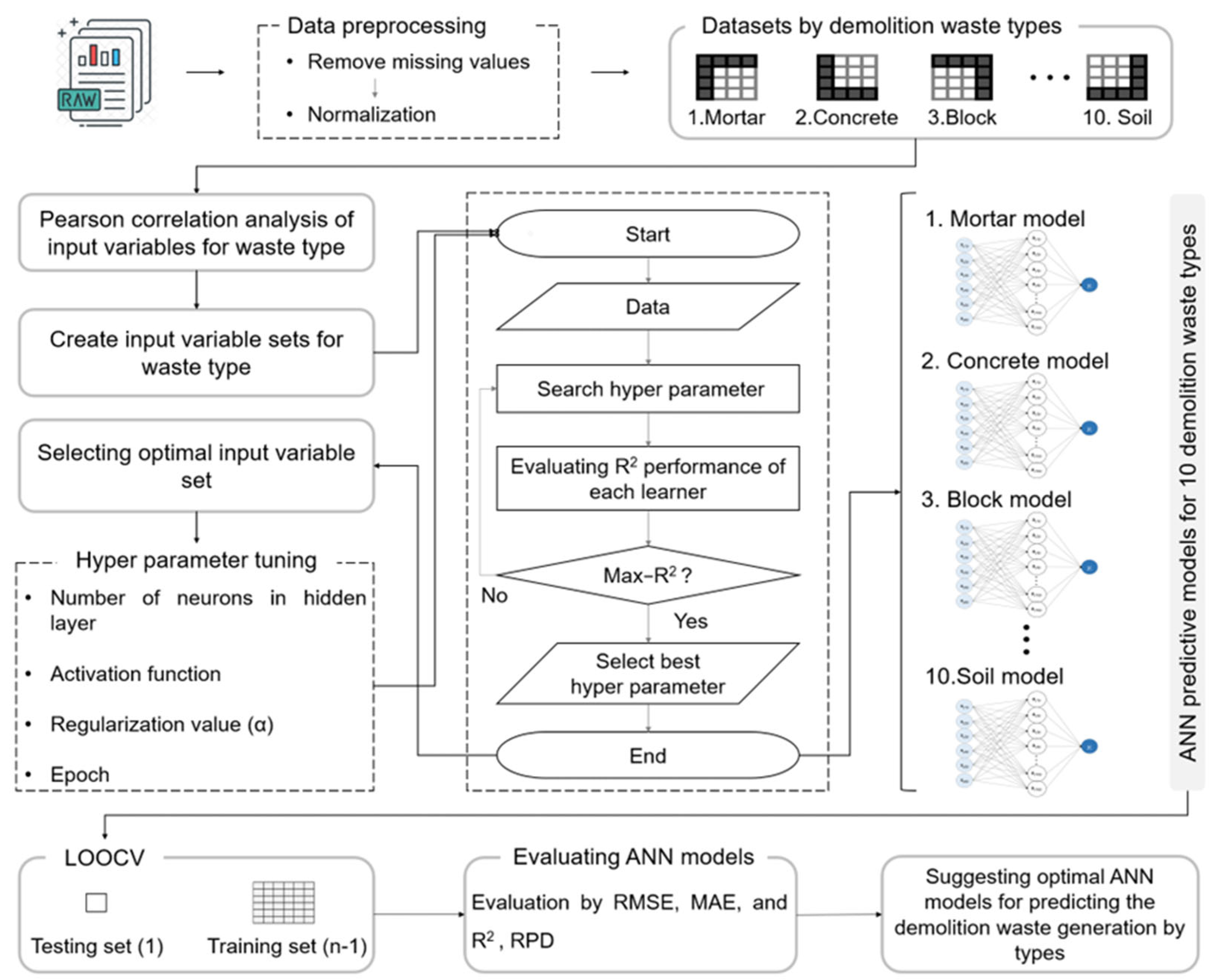
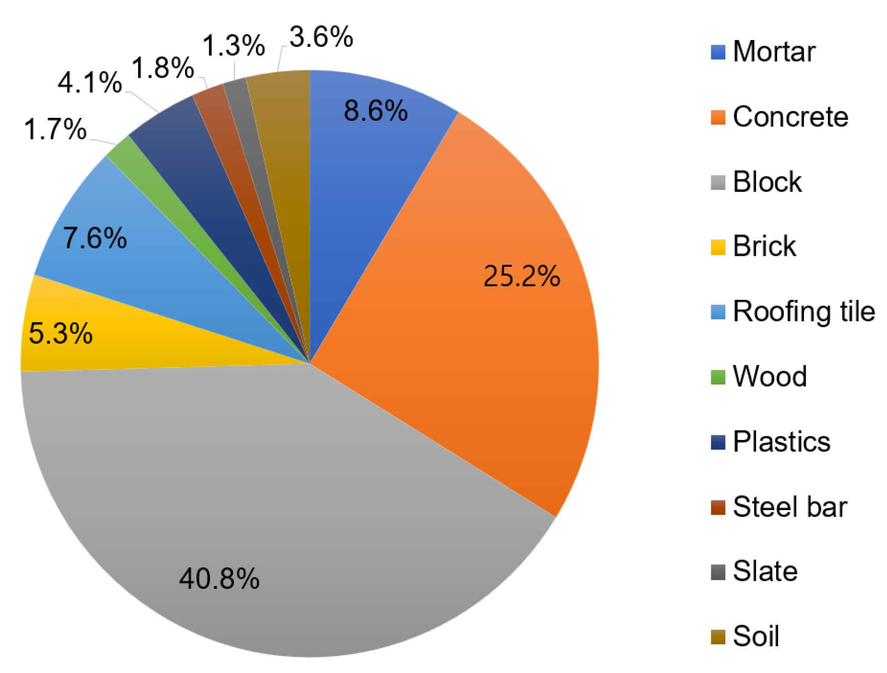
• We collected data on the generation of ten types of DW from 150 old buildings in redevelopment areas, and the raw data were preprocessed to build a dataset.
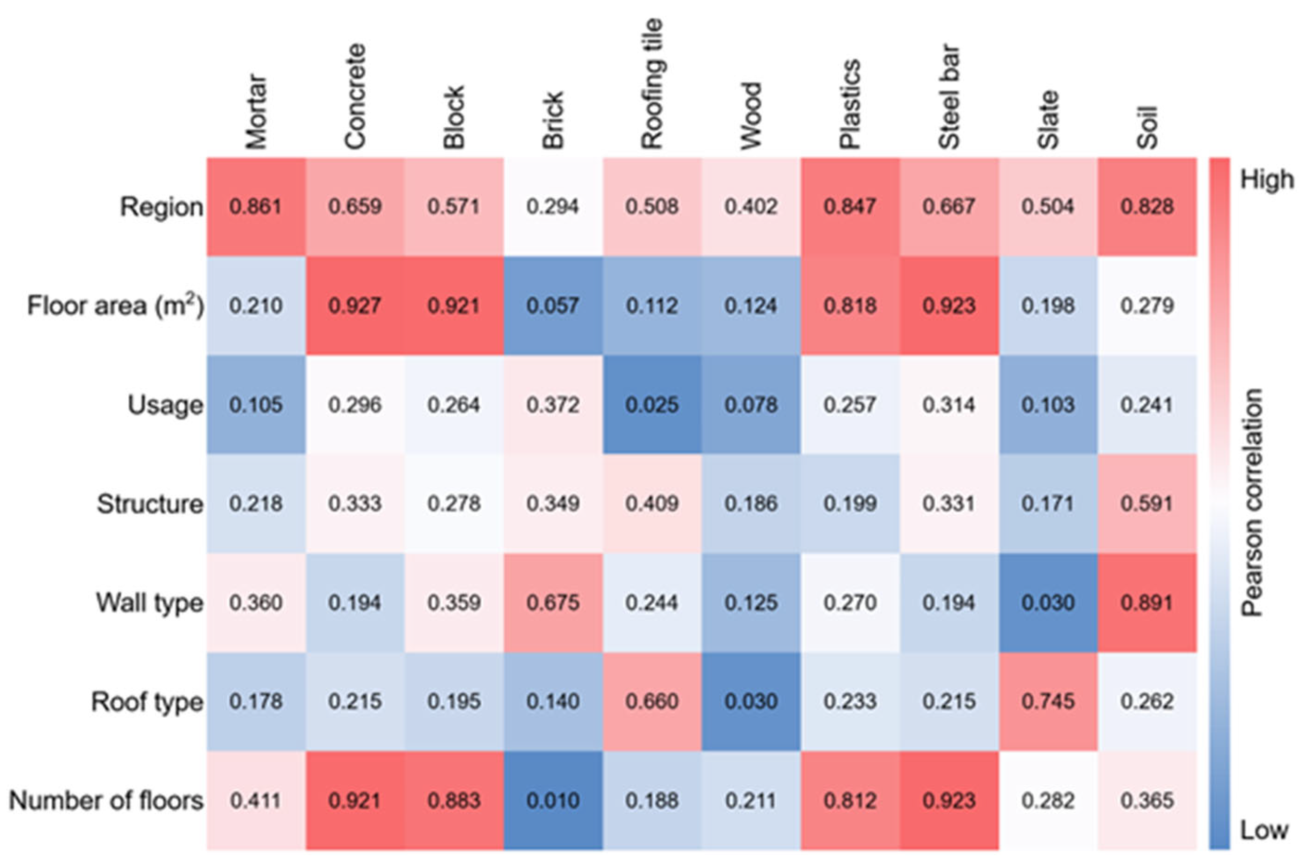
• Variables primarily affecting the generation of each DW type were analyzed.
• An independent set of input variables was developed for each type of DW.
• The ANN algorithm was applied to develop prediction models for each DW type, and the hyperparameters (HPs), including the number of neurons, were adjusted to secure optimal predictive performance for each DW type.
• The leave-one-out cross-validation (LOOCV) technique was used for model development and validation, and the root mean square error (RMSE), coefficient of determination (R²), and mean absolute error (MAE) were used as statistical metrics.
• By evaluating the performance of the developed models, the optimal ANN models for predicting the generation of ten types of DW were proposed.

The remainder of this paper is organized as follows. Section 2 describes the data used to develop and evaluate the ANN models. Section 3 analyzes the performance of the prediction models developed in this study for each DW type. Section 4 compares and discusses the main research findings and existing research results. Finally, Section 5 concludes the study, summarizes its key findings, and discusses its limitations and future research directions.

2. Materials and Methods

This section describes the data used in this study, the data processing methods employed, the development of the DWG prediction models using the ANN algorithm, and the methods adopted for verification and evaluation. Section 2.1 and Section 2.2 describe the data collection and preprocessing method used, including categorical variables. Section 2.3 introduces the ANN algorithm used and its application, correlations between the DW types and input variables, the ANN model structure, and HP adjustments employed to optimize the performance of various DW types. Finally, Section 2.4 describes the verification and evaluation methods employed for the ML models developed for DWG predictions. A flowchart of the model development is shown in Figure 1.

2.1. Data Collection

In this study, the DWG data were collected from the demolition sites in redevelopment areas of Daegu (project A; 81 buildings; 35.88° N, 128.61° E) and Busan (project B; 69 buildings; 35.87° N, 128.63° E), and were recorded as DWG (kg). Before demolition, a direct survey was conducted on 150 buildings to analyze their characteristics (i.e., region, structure, usage, wall type, roof type, gross floor area (GFA), and number of floors) and DWG information for 10 types of waste (i.e., mortar, concrete, block, brick, roofing tile, wood, plastics, steel bar, slate, and soil).

Table 1. Statistical analysis results for the generation of different DW types.

DW Type	Number of Buildings	Maximum DWG (kg)	Minimum DWG (kg)	Average DWG (kg)	Total DWG (kg)	Average DWG Rate (kg·m−2)
Mortar	150	37,329.6	1010.0	13,141.0	1,971,150.4	98.7
Concrete	150	169,481.4	645.1	38,318.7	5,747,801.6	287.8
Block	148	222,621.7	734.4	61,111.3	9,166,689.9	466.8
Brick	104	74,310.1	265.4	6273.8	941,063.4	61.1
Roofing tile	107	17,028.4	4670.1	7474.4	1,121,155.7	87.5
Wood	150	8638.8	663.3	2529.3	379,389.3	19.0
Plastics	150	25,107.5	38.8	6304.8	945,714.0	47.4
Steel bar	150	11,744.9	42.5	2714.2	407,130.4	20.4
Slate	44	6642.7	38.1	659.9	98,980.1	15.0
Soil	64	34,958.4	192.8	2539.6	380,936.8	40.7

presents the statistical analysis results of the type-specific DWG, excluding missing values in the collected data. The amount of waste generated by the demolition of old buildings in redevelopment areas was the highest for block waste at 466.8 kg·m⁻², accounting for 40.8% of the total DW (Figure 2). The amount of concrete was also significant at 287.8 kg·m⁻², accounting for 25.1% of the total DW. Overall, the generated DW comprised 87% minerals (i.e., mortar, concrete, block, brick, and roofing tile) (Figure 2), which is similar to that reported in previous studies [29,30,31]. However, in this study, the generation of block waste was higher than that of concrete, constituting the largest proportion among the 10 DW types, which differed from previous studies [29,30,31,32], wherein concrete generation was reported to be the highest. This is because many old buildings in the redevelopment areas of South Korea have undergone remodeling processes in the past, wherein walls were replaced with blocks [32]. Therefore, predicting DWG based on the information from these old buildings is expected to be useful for future WM in South Korea.

2.2. Data Preprocessing

To improve the prediction performance of AI models, a stable dataset must be constructed. The main purpose of building a stable dataset is to suppress the unwanted impact of distortions or outliers in the data [33,34]. This study preprocessed datasets for each of the 10 DW types to improve the performance of the DW prediction models. Data preprocessing was performed through data standardization to prepare datasets of identical scales as follows:

$$x_{standardization}=\frac{x-\overline{x}}{\sigma },$$

(1)

where $x$ is the element of data, $\overline{x}$ is the mean of the data, and $\sigma$ is the standard deviation of the data.

2.3. Model Development

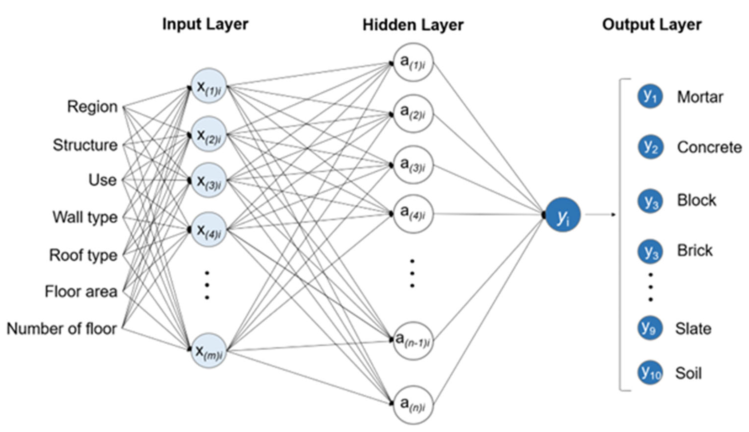
2.3.1. ANN Architecture

ANNs are ML models comprising multiple layers and neurons. They are widely used in the fields of engineering and science for solving complex and challenging problems. ANNs are broadly classified into feedforward and feedback neural networks; feedforward networks have been widely used in engineering fields owing to their relative simplicity and superior performance and are one of the most frequently used algorithms for developing AI models for WM [16,17]. On the other hand, a feedback network is a repetitive network in which information moves in both directions through a loop and is an artificial neural network designed to process temporally continuous data such as time series data. Recurrent neural networks, representative feedback networks, have shown excellent results in time series prediction [35].

The basic structure of an ANN comprises three layers (input, hidden, and output) and nonlinear transfer functions that allow them to learn nonlinear and linear relationships between the input and output neurons, comprising several layers of neurons. Additionally, the ANN structure can be used to realize multilayer perceptron neural networks by expanding the hidden layer.

Because this study aimed to develop ANN models for predicting the generation of ten types of DW, an extremely simple architecture that ensured good performance was required. Therefore, a feedforward neural network with a single hidden layer was adopted. This ANN architecture has been frequently used in WM studies and demonstrated good performance [36,37]. As shown in Figure 3, the ANN architecture comprised up to 7 and 100 neurons in the input and hidden layers, respectively. This architecture was designed to output the resulting values for the ten types of DW in the output layer.

2.3.2. Input Variable Selection for Different Waste Types

Previous studies have reported that CDW generation is significantly affected by the internal factors of buildings, such as type or structure [15,31,37,38,39,40,41], region [32,40,42,43,44,45], use [31,32,38,39,40,46,47], and floor area [30,31,32,38,40,48]. The internal factors of a building are key factors that affect DW generation. Therefore, for predicting the generation of various DW types, appropriate influencing factors must be considered and a suitable set of input variables must be developed for each DW type.

This study employed information regarding the generation of different DW types as well as building features such as region, structure, usage, wall type, roof type, GFA, and the number of floors that affect the generation of different DW types. For this, the Pearson correlation coefficients between the generation of different DW types and building features were analyzed; the results presented in Figure 4 show that DW generation differs significantly based on building features. Specifically, there is a strong correlation between some DW types, such as mortar, concrete, blocks, plastics, steel bars, and soil, in terms of region, floor area, and number of floors. Additionally, certain building features exhibit greater influence on specific DW types. Thus, an input variable set was created to reflect the priority of DW types identified through the Pearson correlation analysis of the building features. Additionally, different combinations of input variables were tested to determine the optimal combination for each DW type, as presented in

Table 2. Input variable sets tested to develop prediction models for different DW types.

DW Type	Input Variable Combination	Number of Input Variables Tested and Combinations of Methods Employed
Mortar	R + N + W + S + F + R.t + U	1, 2, 3, 4, 5, 6, 7 For example, in the case of mortar, the number of input variables was as follows: 1: R 2: R + N 3: R + N + W 4: R + N + W + S 5: R + N + W + S + F 6: R + N + W + S + F + R.t 7: R + N + W + S + F + R.t + U
Concrete	F + N + R + S + U + R.t + W
Block	F + N + R + W + S + U + R.t
Brick	W + U + S + R + R.t + F + N
Roofing tile	R.t + R + S + W + N + F + U
Wood	R + N + S + W + F + U + R.t
Plastics	R + F + N + W + U + R.t + S
Steel bar	F + N + R + S + U + R.t + W
Slate	R.t + R + N + F + S + U + W
Soil	W + R + S + N + F + R.t + U

R: Region, S: structure, U: usage, W: wall type, R.t: roof type, F: floor area, and N: number of floors.

.

2.3.3. HP Tuning

Generally, building an effective ML model is a complex and time-consuming process because it involves appropriate HP tuning for developing an optimal model [49]. The process of designing an optimal model architecture with an optimal HP configuration is called HP tuning, which is a core component that must be considered when building an effective ML model, particularly tree-based models and neural networks with numerous HPs [50]. To prevent overfitting in an ANN model and ensure good prediction performance, we considered two essential HPs: the number of hidden layers and neurons and the type of activation function. Furthermore, to improve the generalizability and reduce training time, appropriate HPs, such as epochs and regularization methods (e.g., learning rate), must be selected [51]. Therefore, we tuned some HPs, including the number of neurons, activation function, learning rate, and number of epochs, with the goals of preventing overfitting, ensuring predictive performance, and reducing the time required for model construction. Additionally, various HP values were tested to determine the model with optimal performance (

Table 3. Network HP specifications used to develop optimal ANN models for different DW types.

HP	Tested Values or Type
Solver	“Adam”, “L-BFGS”, “SGD”
Activation function	“Identity”, “Logistic”, “ReLU”, “Tanh”
Number of neurons in the hidden layer	1, 2, 3, 4, 5, 6, 7, 8, 9,10,12, 14, 16, 18, 20, 24, 26, 28, 30, 40, 50, 60, 70, 80, 90, 100
Learning rate	0.0001, 0.001, 0.01, 0.1 1, 10, 20, 30, 40, 50, 60, 70, 80, 90, 100, 200, 300, 400, 500, 600, 700, 800, 900, 1000
Epochs	10, 20, 30, 40, 50, 60, 70, 80, 90, 100, 120, 140, 160, 180, 200, 500, 1000

L-BFGS: limited-memory Broyden–Fletcher–Goldfarb–Shanno algorithm, SGD: stochastic gradient descent, ReLU: rectified linear unit.

). All experiments were conducted using Python 3.7 and Scikit-learn v1.0 on a computer comprising an AMD Ryzen 7 5800X 8-Core CPU (3.8 GHz, boosting up to 4.7 GHz) and 64 GB RAM.

2.4. Model Testing, Validation, and Evaluation

To develop the DWG prediction models, the data were divided into training and test sets at a ratio of 80:20. When developing a robust ML model, data are generally split into two sets (i.e., training and test), and the data between these sets are typically divided at a ratio of 80:20 [52]. Both sets were generated through uniform random sampling of the preprocessed data [53]. The training set was used to learn the general patterns and features of the dataset, whereas the test set was used to evaluate the performance of the trained model using the optimized HPs obtained during training.

Additionally, the number of samples used to develop the prediction models for different DW types ranged from 44 to 150 (Table 1), which is considered a small sample size. Therefore, we adopted LOOCV to validate the developed model as it is a special case of k-fold cross-validation and is considered suitable for validating small sample sizes [54,55]. In contrast to 10-fold or k-fold cross-validation, LOOCV can validate a small dataset because it uses all samples as test and training data to ensure that a sufficient number of training and validation sets are employed [56,57,58].

Additionally, we adopted MAE, RMSE, and R² as the evaluation metrics for the developed ANN models, which are computed as follows:

$$\mathrm{MAE}=\frac{{{\displaystyle \sum }}_{i=1}^n\left|y_i-x_i\right|}{n},$$

(2)

$$\mathrm{RMSE}=\sqrt{{{\displaystyle \sum }}_{i=1}^n\frac{{\left(y_i-x_i\right)}^2}{n}},$$

(3)

$${\mathrm{R}}^2=1-\frac{{{\displaystyle \sum }}_{i=1}^n{\left(y_i-x_i\right)}^2}{{{\displaystyle \sum }}_{i=1}^n{\left(y_i-{\overline{x}}_i\right)}^2},$$

(4)

where $x_i$, $y_i$, ${\overline{x}}_i$, and ${\overline{y}}_i$ are the observed, predicted, average observed, and average predicted quantities of the generated DWs, respectively, and n is the number of samples. A satisfactory model generally yields high R² values and low MAE, MSE, and RMSE values.

Additionally, the ML model performance must be validated through a multi-criteria process to ensure that its accuracy is not exaggerated or distorted [59,60]. In addition to evaluating the performance using single metrics such as MAE, RMSE, and R², the ratio of percent deviation (RPD) was also considered a complementary performance indicator. The RPD was calculated using Equation (5), and performance classification according to the RPD value is presented in

Table 4. Model performance classification based on RPD values.

RPD Values	Performance Indicator	Remarks
RPD < 1	Very poor	Model/predictions whose use is not recommended
1 $\le$ RPD $<$ 1.4	Poor	Model/predictions where only high and low values are distinguishable
1.4 $\le$ RPD $<$ 1.8	Fair	Model/predictions which may be used for assessment and correlation
1.8 $\le$ RPD $<$ 2	Good	Model/predictions where quantitative predictions are possible
2 $\le$ RPD $<$ 2.5	Very good	Quantitative model/ predictions

[60].

$$\mathrm{RPD}=\frac{Standard deviation}{RMSE}.$$

(5)

3. Results

3.1. Optimal HP Values and Input Variable Sets for Various DW Types

A wide range of HP values and input variable sets were tested to develop optimal DWG prediction models for different DW types, and the resulting optimal HPs are listed in

Table 5. Optimal HP values and input variable sets for different waste types to predict DWG.

DW Type	HP				Input Variable Set
	Activation Function	Number of Neurons in Hidden Layer	Learning Rate	Epochs
Mortar	Identity	20	600	50	R + N + W + S + F + R.t + U
	Logistic	10	1	60	R + N + W + S
	Tanh	16	1	1000	R + N + W + S + F
	ReLU	4	0.1	60	R + N + W + S + F + R.t + U
Concrete	Identity	1	30	50	F + N + R + S + U + R.t + W
	Logistic	18	0.1	60	F
	Tanh	10	1	120	F + N
	ReLU	5	0.0001	50	F + N + R + S + U + R.t + W
Block	Identity	2	1	20	F + N + R + W
	Logistic	4	0.01	40	F
	Tanh	10	1	100	F + N
	ReLU	5	1	40	F + N + R + W + S + U
Brick	Identity	4	10	30	W + U + S
	Logistic	60	1	200	W + U + S + R
	Tanh	40	1	40	W + U + S + R
	ReLU	4	0.0001	50	W + U + S + R + R.t + F
Roofing tile	Identity	2	1	30	R.t + R + S + W + N + F
	Logistic	70	1	120	R.t + R + S + W + N + F + U
	Tanh	60	1	20	R.t + R + S
	ReLU	10	100	50	R.t + R + S + W + N + F
Wood	Identity	8	10	20	R + N + S + W + F + U + R.t
	Logistic	90	1	1000	R + N + S + W + F + U + R.t
	Tanh	26	0.1	120	R + N + S + W + F + U
	ReLU	50	0.01	60	R + N + S + W + F + U
Plastics	Identity	1	0.0001	20	R + F + N + W + U + R.t + S
	Logistic	18	1	500	R + F + N
	Tanh	50	0.01	120	R + F + N
	ReLU	10	1	50	R + F
Steel bar	Identity	7	100	40	F + N + R + S + U + R.t
	Logistic	6	1	70	F
	Tanh	18	0.1	50	F + N + R
	ReLU	3	1	50	F + N + R + S + U + R.t + W
Slate	Identity	16	0.0001	30	F + N + R + S + U
	Logistic	3	1	30	F
	Tanh	60	1	50	F
	ReLU	10	0.001	40	F + N + R + S
Soil	Identity	1	0.0001	10	W
	Logistic	3	1	180	W
	Tanh	2	1	50	W
	ReLU	6	0.1	60	W + R + S + N + F

. The “solver” that is not included in Table 5 was tested against Adam, L-BFGS, and SGD. Because L-BFGS showed superior performance compared to Adam and SGD, only the results for L-BFGS are included in Table 5. For different DW types, the optimal HP values of the ANN models for DWG predictions varied according to the activation function; thus, various HP values were selected. In particular, most models had fewer than 20 neurons in the hidden layer and involved ≤200 epochs. This simple structure and low calculation count were considered efficient and cost-effective for model development. Additionally, we tested various combinations of input variables for different DW types, and each model yielded different optimal combinations, comprising one to seven input variables. These results suggest that input variable selection is crucial for ANN models and depends on the type of activation function employed. Moreover, it is essential to develop an appropriate set of input variables based on the selected HPs.

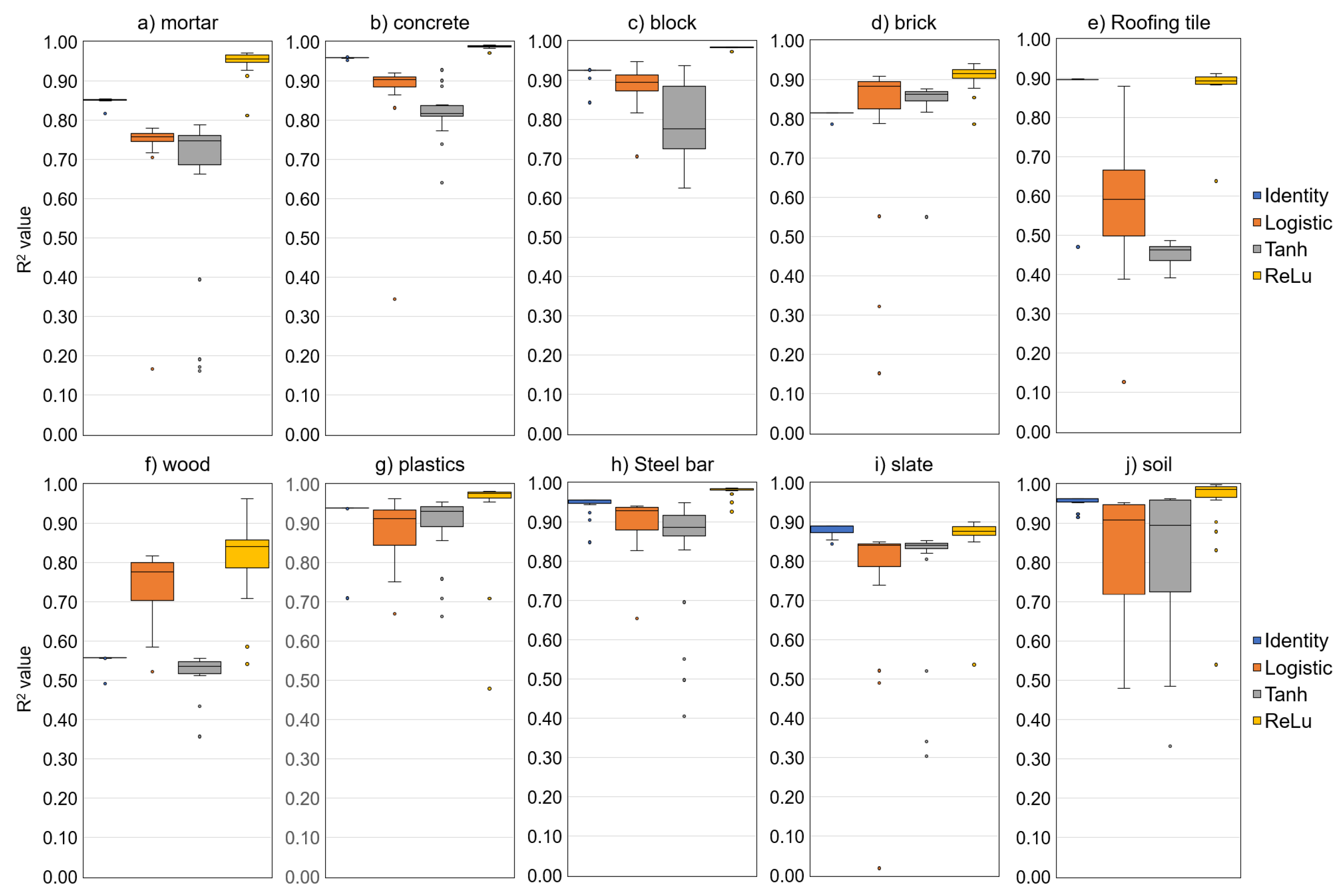
3.2. Model Performance According to Waste Type

The performance results (R²) of all the sub-models tested for developing an optimal ANN prediction model for the 10 types of DW are shown in Figure 5. The R² values varied significantly for different DW types, depending on the type of activation function employed. However, the ANN models using ReLU generally exhibited the best prediction performance for all DW types. In contrast, the “identity” function exhibited stable results and little variation in performance regardless of other HP values (i.e., number of neurons, learning rate, and epochs). However, the logistic and tanh functions showed considerable variations in prediction performance based on the number of neurons, learning rate, and epochs. Additionally, they sometimes exhibited high variations, such as in the case of blocks, roofing tiles, and soil, and low variations, such as in the case of mortar, roofing tiles, wood, and soil. These variations indicate that the models were not stable. Therefore, ReLU is considered appropriate for developing the most accurate and stable DWG prediction model for the ten DW types. The results (

Table 6. DWG prediction performance of the ANN models for different DW types.

DW Type	Activation Function	Performance Metrics
		Validation			Test
		RMSE	MAE	R2	RMSE	MAE	R2
Mortar	Identity	2692.4	1774.7	0.895	3191.4	2035.6	0.852
	Logistic	3971.4	2760.3	0.771	3877.6	2581.3	0.781
	Tanh	3053.1	1728.1	0.864	3222.5	2243.6	0.849
	ReLU	1059.8	744.0	0.984	1440.5	1007.7	0.970
Concrete	Identity	8778.2	6704.6	0.972	10,572.3	7721.8	0.959
	Logistic	19,882.1	13116.7	0.855	12,624.7	9963.8	0.942
	Tanh	11,787.3	9524.4	0.949	11,459.2	9090.2	0.952
	ReLU	3347.1	2341.4	0.996	4762.4	3153.2	0.992
Block	Identity	16,887.6	11,497.5	0.940	18,706.7	12,268.5	0.927
	Logistic	21,817.7	13,618.1	0.900	15,756.6	12,663.9	0.948
	Tanh	13,919.2	10,759.3	0.959	16,050.4	12,551.8	0.946
	ReLU	7353.4	5202.4	0.989	8589.5	6170.2	0.985
Brick	Identity	6022.1	3139.2	0.869	7116.0	3593.0	0.817
	Logistic	4486.9	2176.3	0.927	5016.0	2517.0	0.909
	Tanh	6562.4	3250.4	0.845	5856.2	2840.3	0.876
	ReLU	2108.9	986.3	0.984	4017.8	1838.1	0.942
Roofing tile	Identity	819.6	649.0	0.915	897.0	702.1	0.898
	Logistic	562.6	416.2	0.960	970.6	732.4	0.881
	Tanh	2070.9	1639.7	0.458	1988.7	1540.9	0.500
	ReLU	729.6	579.0	0.933	835.4	671.9	0.912
Wood	Identity	906.7	612.5	0.620	977.4	671.8	0.559
	Logistic	253.7	162.1	0.970	630.0	438.4	0.817
	Tanh	580.5	407.0	0.844	979.2	661.8	0.557
	ReLU	434.2	325.9	0.913	548.4	413.9	0.861
Plastics	Identity	1581.8	1211.7	0.951	1752.7	1329.9	0.940
	Logistic	2450.6	1041.4	0.883	1378.1	852.5	0.963
	Tanh	2144.9	1136.4	0.910	1534.1	889.0	0.954
	ReLU	901.3	571.6	0.984	998.1	629.7	0.981
Steel bar	Identity	648.8	502.1	0.969	747.5	558.5	0.959
	Logistic	1263.7	845.6	0.883	891.8	736.6	0.942
	Tanh	1059.3	603.0	0.918	894.9	525.5	0.941
	ReLU	343.9	212.9	0.991	426.9	266.7	0.987
Slate	Identity	671.4	487.2	0.921	791.4	593.8	0.890
	Logistic	965.4	774.3	0.836	921.8	707.7	0.851
	Tanh	868.8	630.7	0.867	915.6	667.9	0.853
	ReLU	625.8	431.8	0.931	744.8	536.5	0.902
Soil	Identity	1699.3	1494.5	0.967	1784.6	1568.1	0.963
	Logistic	2180.2	1759.9	0.945	1969.5	1674.3	0.955
	Tanh	1736.3	1474.4	0.965	1783.6	1477.8	0.963
	ReLU	447.3	375.1	0.998	845.4	549.9	0.992

) of the optimal prediction models, incorporating HPs from Table 5, for each activation function type. The validation results indicated that logistic regression obtained the best prediction performance for roofing tiles and wood, with R² values of 0.960 and 0.970, respectively, whereas ReLU performed the best for other DW types. However, the test results showed that the prediction performance of ReLU was the best for all DW types. The ANN models employing ReLU exhibited an average R² of 0.970, RMSE of 1735.1, and MAE of 1177.0 for the validation results, and R² of 0.952, RMSE of 2320.9, and MAE of 1523.8 for the test results. These results indicate that ANN models employing ReLU have superior prediction performance compared to those employing other activation functions. Consequently, the ANN model with ReLU was considered the most suitable for predicting all 10 types of DW.

3.3. Prediction Results of Optimal Models

Table 7. Structure and performance results of optimal models for DWG prediction for different waste types.

DW Type	ANN Model Structure (Input Layer–Hidden Layer–Output Layer)	RPD Value		Performance Indicator
		Validation	Test	Validation	Test
Mortar	7-4-1	7.8	5.7	Excellent	Excellent
Concrete	7-5-1	15.6	10.9	Excellent	Excellent
Block	6-5-1	9.3	8.0	Excellent	Excellent
Brick	6-4-1	7.9	4.2	Excellent	Excellent
Roofing tile	6-10-1	3.7	3.4	Excellent	Excellent
Wood	6-50-1	3.2	2.6	Excellent	Excellent
Plastics	2-10-1	7.8	7.1	Excellent	Excellent
Steel bar	7-3-1	10.7	8.6	Excellent	Excellent
Slate	4-10-1	3.7	3.1	Excellent	Excellent
Soil	5-6-1	20.8	11.0	Excellent	Excellent

presents the test and validation results of the optimal ANN models for predicting the generation (kg) of the ten DW types. The validation results (RPD) of the ANN model for DWG prediction indicate excellent predictive performance, with values ≥ 3.2 for all waste types. The test results also indicate excellent predictive performance for all waste types, with RPD values ≥ 2.6. Among the waste types, the models for soil (RPD values: validation = 20.8, test = 11.0) and concrete (RPD values: validation = 15.6, test = 10.9) exhibited the best performance, whereas those for wood, slate, and roofing tiles exhibited relatively low performance compared with those for other waste materials. Nevertheless, the test and validation results showed that the RPD of all prediction models was ≥2.5, indicating excellent performance. Furthermore, as shown in Figure 6, the test results for the concentration values between the observed and predicted values of the ten DWG prediction models indicate that the concentration values of all DWG models are concentrated on the centerline (observed value = predicted value), which indicates that the predicted values are close to the observed values, again demonstrating excellent performance.

To develop a prediction model for ten types of DW, maximizing the simplicity of the model structure can help reduce the development cost and time. Therefore, the optimal ANN model developed in this study had a simple structure with only one hidden layer (Table 7), and the number of neurons in the hidden layer was ≤10 for all models except that of wood. Moreover, all respective models developed for the ten DW types exhibited excellent prediction performance, indicating that they can be used for DWG predictions.

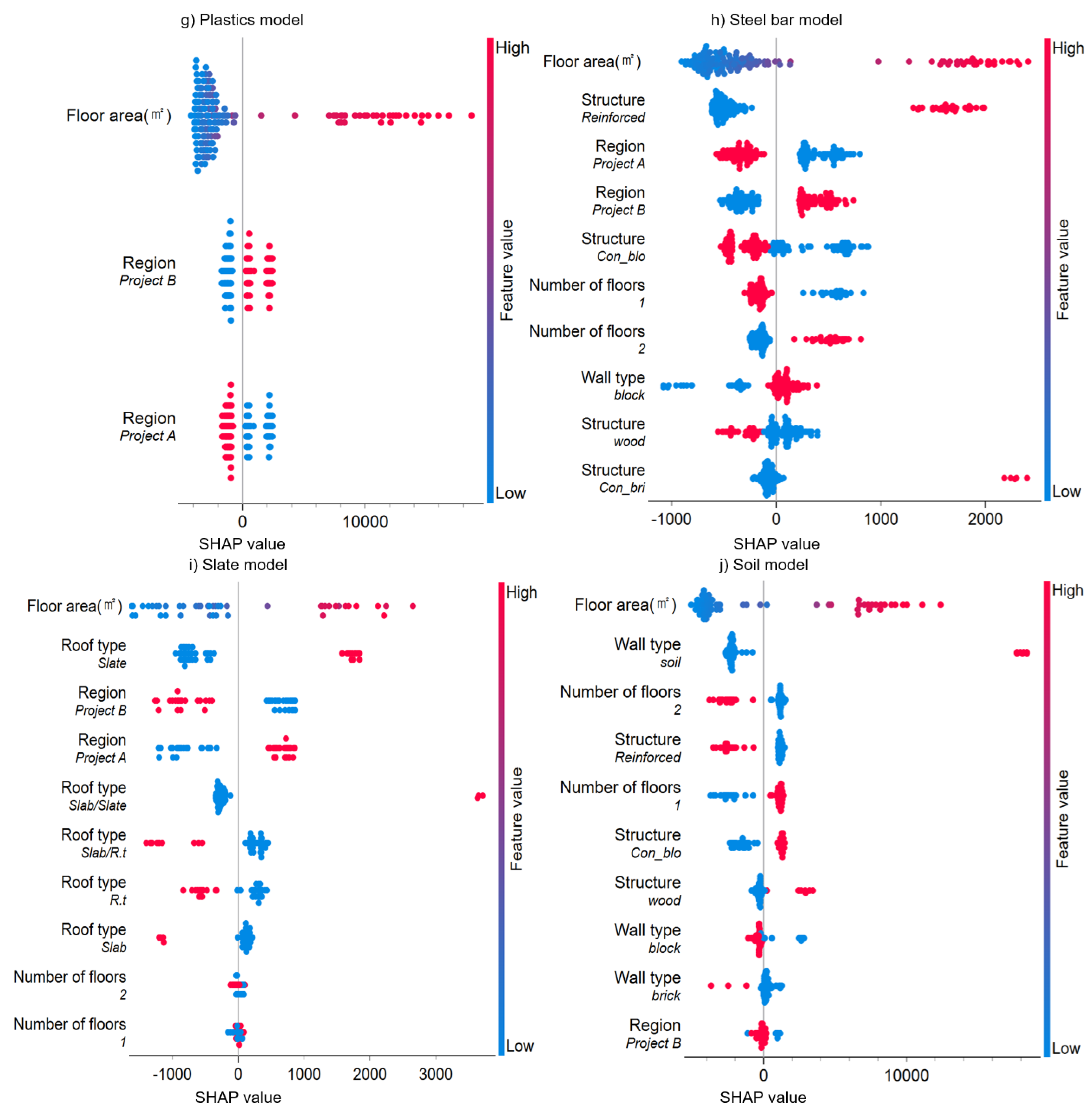
3.4. Key Input Variables of Prediction Models

This study analyzed the significance of the input variables for the ten DWG prediction models using the Shapley additive explanations (SHAP) method, which is used to quantify the significance of input variables [61,62]. It is used to identify the contributions of input variables to the final model prediction and can be used to improve model performance and interpretability [63]. In ML models, the SHAP algorithm calculates the contribution of each input variable to the final prediction by averaging the contributions of all possible combinations of the input variables. A SHAP value close to zero indicates that the corresponding input variable does not significantly contribute to the model prediction.

Figure 7 shows the ranking of the main input variables affecting the predictions of the ten DW types, wherein it is evident that the impacts of the input variables on the DWG models vary considerably depending on the DW type, with the following characteristics being the most important:

• Floor area: Overall, this input variable most critically affected DWG and ranked the highest for nine (excluding the brick model) of the ten DWG models. Additionally, it showed a strong positive impact on DWG predictions of all models.
• Region: This input variable had a high impact on DWG prediction, and its correlations with DWG predictions varied. For example, in the mortar and slate models, one region (project A) showed a positive correlation, whereas another region (project B) showed a negative impact. The other DW types also showed contrasting results.
• Structure: This variable showed varying correlations depending on the DW type; it (reinforce) showed a negative correlation with the generation of mortar, roofing tiles, wood, and soil but a positive correlation with that of concrete, blocks, and steel bars. Additionally, various correlations were also observed between DW type and DWG in other structures (con_bri, con_blo, and wood).
• Wall type: This variable had the most significant impact on brick generation, with a positive correlation when the wall type was brick. Conversely, when the wall type was block, a negative correlation with brick generation was observed. These results contrast with the effects of wall type on block generation in the block model.
• Number of floors, usage, and roof type: The number of floors appeared to affect the generation of concrete, blocks, roofing tiles, wood, and steel bars; however, its SHAP values were not large. The “number of floors_1” showed a positive correlation with the generation of roofing tiles and wood and a negative correlation with that of concrete, blocks, and steel bars. Furthermore, “number of floors_2” showed the opposite correlation with “number of floors_1.” Additionally, usage affected brick generation; however, its impact was not significant. The brick model shown in Figure 7d indicates that brick generation varies with usage type. Finally, roof type was an important input variable in the mortar, concrete, brick, and roofing tile models; however, its SHAP values were not large.

4. Discussion

Developing prediction models for various types of DW is challenging, primarily because each waste type has different characteristics, and individual factors must be pre-analyzed to reflect them. Research on the management of various types of waste has been actively conducted in the MSW and CDW fields. Adeleke et al. [26] developed prediction models for different types of MSW, including organic, paper, plastic, and textile, using ANNs, and their predictive performance (R²) ranged from 0.826 to 0.916. They used maximum temperature, minimum temperature, wind speed, and humidity as input variables for all four prediction models. Golbaz et al. [27] developed a prediction model for infectious, general, and total hospital solid waste using an ANN algorithm and seven input variables and achieved test and validation performance (R²) of 0.64 and 0.76, respectively. Kumar et al. [19] developed an ANN model using education, occupation, income, and type of house as input variables for predicting various types of plastic waste generated in the city of Dhanbad, India; their model achieved an R² value of 0.75. Kannangara et al. [28] developed prediction models for MSW and paper generation in Ontario, Canada, using an ANN algorithm and seven socioeconomic input variables. Their prediction model with five socioeconomic input variable sets showed the best performance, with the best test R² values of 0.72 and 0.35 for MSW and paper, respectively. The aforementioned studies are examples of those that developed models with simple ANN structures for predicting various waste types. However, the prediction performances of these models vary according to the type of waste. It should be noted that these studies employed the same set of input variables for various types of waste, which did not sufficiently reflect the factors affecting each waste type. In other words, independent sets of input variables were not developed for different types of waste, which may have partially resulted in their low prediction performance. From this perspective, we believe that developing independent input variable sets through a proper impact factor analysis is crucial for developing ML-based prediction models for various waste types. Therefore, this study can be seen as suggesting specialized modeling methods for each type of DW that were not presented in existing studies [19,26,27,28]. This approach is differentiated from existing studies by selecting variables that reflect the unique characteristics of each type of DW, enabling the development of a more specialized set of input variables and a DW prediction model with improved accuracy. As is evident from

Table 8. Comparison of studies on ANN prediction models for various waste types.

Study	Waste Type	Whether Individual Sets of Input Parameters Were Developed for Each Waste Type	Performance (R2) of Prediction Models
This study	Mortar Concrete Block Brick Roofing tile Wood Plastics Steel bar Slate Soil	Yes	Test: 0.861–0.991; Validation: 0.913–0.998
[26]	Organic Paper Plastic Textile	No	0.826–0.916
[27]	Infectious hospital solid waste General hospital solid waste Total hospital solid waste	No	Test: 0.58–0.64; Validation: 0.66–0.78
[19]	Plastics	No	0.75
[28]	MSW Paper	No	0.72 0.35

, this study differs from existing research in that it developed individual input variable sets for the ten types of DW and constructed DWG prediction models with a simple structure and excellent predictive performance.

This study analyzed the factors influencing the predictions of the ten types of DW using SHAP values. Floor area was identified as the most important factor affecting the generation of all types of waste, demonstrating a strong positive correlation. Previous studies [25,38,64] have also found that floor area is a major input variable affecting DWG. Additionally, other building characteristics (building type or usage, structure, element type, region, etc.) were also shown to be major factors influencing DWG. However, in this study, the results for the building characteristics, such as building type or usage, structure, element type, and region, across the ten types of DWG models differed from those obtained in previous studies. For example, building characteristics other than floor area exhibited a positive correlation with the generation of some DW types and a negative correlation with that of others. The SHAP values indicated the existence of complex relationships between building characteristics and the generation of different DW types. Based on these findings, we believe that the development of good prediction models for various DW types requires the simultaneous development of an optimal set of input variables using various input variable combinations. Furthermore, AI tools, such as the SHAP value, are extremely useful for developing good prediction models for WM and understanding the characteristics of waste types.

5. Conclusions

This study aimed to understand the characteristics of various DW types from buildings in redevelopment areas in South Korea and develop DWG prediction models for ten types of DW. We applied an ANN algorithm, derived the optimal set of input variables and HP adjustments for each of the ten DW types, and then developed optimal DWG prediction models for each DW type. Additionally, individual input variable sets were developed for the ten DW types, and individual ANN models were implemented by deriving the optimal HP values. The DWG prediction models exhibited high R² values, ranging from 0.913 (wood model) to 0.998 (soil model) for the validation results and from 0.861 (wood model) to 0.992 (concrete and soil models) for the test results. Furthermore, the RPD for all DWG models was ≥2.5, indicating that they exhibited excellent prediction performance. Most of the proposed ANN models had simple structures comprising 3–10 neurons in the hidden layer; thus, they are considered efficient in terms of development time and cost.

Furthermore, the factors affecting the generation of the ten DW types were analyzed through SHAP. The floor area was found to have the strongest positive correlation with DWG and the most significant impact on the generation of all DW types. In contrast, other factors (region, number of floors, structure, usage, and wall type) showed either a positive or negative correlation with DWG, depending on the DW type. These results indicate that certain variables are more significant or have different relationships with other variables depending on the DW type, and the DWG predictions are affected by more complex factors than expected. Therefore, AI technology is highly useful for analyzing these factors, and the results of this study may be significant for selecting input variables to develop future DWG prediction models.

The ten DWG prediction models developed in this study can be effectively used for efficient WM. From an economic perspective, the results of this study can help promote effective resource utilization and reduce costs. Demolition companies can use accurate DWG results for each waste type to allocate demolition personnel, appropriate number of trucks, handling costs, and recycling plans, which can enhance their efficiency, cost savings, and resource management. Additionally, from a commercial perspective, it can be useful in creating business opportunities through reselling recyclable resources. Additionally, in terms of public policy, it can be used to derive effective waste management policies through accurate predictions for each type of DW. Central and local governments can utilize accurate DWG data for landfill management, identifying waste disposal facility capacity, efficiently operating recycling facilities, and urban planning by considering the location and capacity of waste disposal facilities. This can support effective decision-making for efficient DW management and resource allocation. Additionally, this can be useful for the government to decide on measures for specific waste. Lastly, from a social perspective, the results of this study can reduce environmental costs through efficient waste management, thereby increasing environmental awareness and showing that waste management is closely related to the environment and the economy. However, the application of this research result requires investment and cooperation from the government or companies. In addition, for field application, training for related experts and workers and awareness of the usefulness of waste management using AI are required.

The ANN-based prediction models developed in this study for the ten DW types comprised simple structures and exhibited high prediction performance. The simple ANN structure offers advantages such as overfitting prevention, improved generalizability, and quick learning and predictions. However, the wood model (validation and test R² values of 0.913 and 0.861, respectively) had as many as 50 neurons in the hidden layer and exhibited a relatively low prediction performance compared with the other DW models. Because other DW models yielded excellent performance results under the same conditions, this cannot be easily attributed to data preprocessing problems, insufficient data, or overfitting. The findings of this study indicate that appropriate input variables must be employed to develop a model for wood with better performance. Therefore, to address this research limitation, future work should aim to develop an improved DWG prediction model by employing additional input variables.

References

1. Karak, T.; Bhagat, R.M.; Bhattacharyya, P. Municipal Solid Waste Generation, Composition, and Management: The World Scenario. Crit. Rev. Environ. Sci. Technol. 2012, 42, 1509–1630. [Google Scholar] [CrossRef]
2. Gallardo, A.; Carlos, M.; Colomer, F.; Edo-Alcón, N. Analysis of the Waste Selective Collection at Drop-off Systems: Case Study Including the Income Level and the Seasonal Variation. Waste Manag. Res. 2018, 36, 30–38. [Google Scholar] [CrossRef] [PubMed]
3. Pathak, D.R.; Mainali, B.; Abuel-Naga, H.; Angove, M.; Kong, I. Quantification and Characterization of the Municipal Solid Waste for Sustainable Waste Management in Newly Formed Municipalities of Nepal. Waste Manag. Res. 2020, 38, 1007–1018. [Google Scholar] [CrossRef]
4. Yuan, H.; Shen, L. Trend of the Research on Construction and Demolition Waste Management. Waste Manag. 2011, 31, 670–679. [Google Scholar] [CrossRef]
5. Park, J.; Tucker, R. Overcoming Barriers to the Reuse of Construction Waste Material in Australia: A Review of the Literature. Int. J. Constr. Manag. 2017, 17, 228–237. [Google Scholar] [CrossRef]
6. Hassan, S.H.; Hamidi, A.A.; Izwan, J.; Yung-Tse, H. Construction and Demolition (C&D) Waste Management and Disposal. In Solid Waste Engineering and Management; Springer: Cham, Switzerland, 2022; pp. 165–216. [Google Scholar]
7. Wu, H.; Zuo, J.; Zillante, G.; Wang, J.; Yuan, H. Status Quo and Future Directions of Construction and Demolition Waste Research: A Critical Review. J. Clean. Prod. 2019, 240, 118163. [Google Scholar] [CrossRef]
8. López Ruiz, L.A.; Roca Ramón, X.; Gassó Domingo, S. The Circular Economy in the Construction and Demolition Waste Sector—A Review and an Integrative Model Approach. J. Clean. Prod. 2020, 248, 119238. [Google Scholar] [CrossRef]
9. Butera, S.; Christensen, T.H.; Astrup, T.F. Composition and Leaching of Construction and Demolition Waste: Inorganic Elements and Organic Compounds. J. Hazard. Mater. 2014, 276, 302–311. [Google Scholar] [CrossRef]
10. Lu, W.; Yuan, H.; Li, J.; Hao, J.J.L.; Mi, X.; Ding, Z. An Empirical Investigation of Construction and Demolition Waste Generation Rates in Shenzhen City, South China. Waste Manag. 2011, 31, 680–687. [Google Scholar] [CrossRef]
11. Katz, A.; Baum, H. A Novel Methodology to Estimate the Evolution of Construction Waste in Construction Sites. Waste Manag. 2011, 31, 353–358. [Google Scholar] [CrossRef]
12. Nagapan, S.; Rahman, I.A.; Asmi, A.; Adnan, N.F. Study of Site’s Construction Waste in Batu Pahat, Johor. Procedia Eng. 2013, 53, 99–103. [Google Scholar] [CrossRef]
13. Kartam, N.; Al-Mutairi, N.; Al-Ghusain, I.; Al-Humoud, J. Environmental Management of Construction and Demolition Waste in Kuwait. Waste Manag. 2004, 24, 1049–1059. [Google Scholar] [CrossRef] [PubMed]
14. Wijewickrama, M.K.C.S.; Chileshe, N.; Rameezdeen, R.; Ochoa, J.J. Information Sharing in Reverse Logistics Supply Chain of Demolition Waste: A Systematic Literature Review. J. Clean. Prod. 2021, 280, 124359. [Google Scholar] [CrossRef]
15. Cheng, J.C.P.; Ma, L.Y.H. A BIM-Based System for Demolition and Renovation Waste Estimation and Planning. Waste Manag. 2013, 33, 1539–1551. [Google Scholar] [CrossRef] [PubMed]
16. Abdallah, M.; Abu Talib, M.; Feroz, S.; Nasir, Q.; Abdalla, H.; Mahfood, B. Artificial Intelligence Applications in Solid Waste Management: A Systematic Research Review. Waste Manag. 2020, 109, 231–246. [Google Scholar] [CrossRef] [PubMed]
17. Xu, A.; Chang, H.; Xu, Y.; Li, R.; Li, X.; Zhao, Y. Applying Artificial Neural Networks (ANNs) to Solve Solid Waste-Related Issues: A Critical Review. Waste Manag. 2021, 124, 385–402. [Google Scholar] [CrossRef] [PubMed]
18. Wang, D.; He, H.; Liu, D. Intelligent Optimal Control with Critic Learning for a Nonlinear Overhead Crane System. IEEE Trans. Ind. Inform. 2017, 14, 2932–2940. [Google Scholar] [CrossRef]
19. Kumar, A.; Samadder, S.R.; Kumar, N.; Singh, C. Estimation of the Generation Rate of Different Types of Plastic Wastes and Possible Revenue Recovery from Informal Recycling. Waste Manag. 2018, 79, 781–790. [Google Scholar] [CrossRef]
20. Soni, U.; Roy, A.; Verma, A.; Jain, V. Forecasting Municipal Solid Waste Generation Using Artificial Intelligence Models—A Case Study in India. SN Appl. Sci. 2019, 1, 162. [Google Scholar] [CrossRef]
21. Wu, F.; Niu, D.; Dai, S.; Wu, B. New Insights into Regional Differences of the Predictions of Municipal Solid Waste Generation Rates Using Artificial Neural Networks. Waste Manag. 2020, 107, 182–190. [Google Scholar] [CrossRef]
22. Hoque, M.M.; Rahman, M.T.U. Landfill Area Estimation Based on Solid Waste Collection Prediction Using ANN Model and Final Waste Disposal Options. J. Clean. Prod. 2020, 256, 120387. [Google Scholar] [CrossRef]
23. Ayeleru, O.O.; Fajimi, L.I.; Oboirien, B.O.; Olubambi, P.A. Forecasting Municipal Solid Waste Quantity Using Artificial Neural Network and Supported Vector Machine Techniques: A Case Study of Johannesburg, South Africa. J. Clean. Prod. 2021, 289, 125671. [Google Scholar] [CrossRef]
24. Jassim, M.S.; Coskuner, G.; Zontul, M. Comparative Performance Analysis of Support Vector Regression and Artificial Neural Network for Prediction of Municipal Solid Waste Generation. Waste Manag. Res. 2022, 40, 195–204. [Google Scholar] [CrossRef]
25. Cha, G.-W.; Choi, S.-H.; Hong, W.-H.; Park, C.-W. Development of Machine Learning Model for Prediction of Demolition Waste Generation Rate of Buildings in Redevelopment Areas. Int. J. Environ. Res. Public Health 2022, 20, 107. [Google Scholar] [CrossRef] [PubMed]
26. Adeleke, O.; Akinlabi, S.A.; Jen, T.-C.; Dunmade, I. Application of Artificial Neural Networks for Predicting the Physical Composition of Municipal Solid Waste: An Assessment of the Impact of Seasonal Variation. Waste Manag. Res. 2021, 39, 1058–1068. [Google Scholar] [CrossRef] [PubMed]
27. Golbaz, S.; Nabizadeh, R.; Sajadi, H.S. Comparative Study of Predicting Hospital Solid Waste Generation Using Multiple Linear Regression and Artificial Intelligence. J. Environ. Health Sci. Eng. 2019, 17, 41–51. [Google Scholar] [CrossRef] [PubMed]
28. Kannangara, M.; Dua, R.; Ahmadi, L.; Bensebaa, F. Modeling and Prediction of Regional Municipal Solid Waste Generation and Diversion in Canada Using Machine Learning Approaches. Waste Manag. 2018, 74, 3–15. [Google Scholar] [CrossRef]
29. Kleemann, F.; Lederer, J.; Aschenbrenner, P.; Rechberger, H.; Fellner, J. A Method for Determining Buildings’ Material Composition Prior to Demolition. Build. Res. Inf. 2016, 44, 51–62. [Google Scholar] [CrossRef]
30. Wu, H.; Duan, H.; Zheng, L.; Wang, J.; Niu, Y.; Zhang, G. Demolition Waste Generation and Recycling Potentials in a Rapidly Developing Flagship Megacity of South China: Prospective Scenarios and Implications. Constr. Build. Mater. 2016, 113, 1007–1016. [Google Scholar] [CrossRef]
31. Yu, B.; Wang, J.; Li, J.; Zhang, J.; Lai, Y.; Xu, X. Prediction of Large-Scale Demolition Waste Generation during Urban Renewal: A Hybrid Trilogy Method. Waste Manag. 2019, 89, 1–9. [Google Scholar] [CrossRef]
32. Cha, G.-W.; Kim, Y.-C.; Moon, H.J.; Hong, W.-H. New Approach for Forecasting Demolition Waste Generation Using Chi-Squared Automatic Interaction Detection (CHAID) Method. J. Clean. Prod. 2017, 168, 375–385. [Google Scholar] [CrossRef]
33. Kuhn, M.; Johnson, K. Applied Predictive Modeling; Springer: New York, NY, USA, 2013; ISBN 978-1-4614-6848-6. [Google Scholar]
34. Nisbet, R.; Elder, J.; Miner, G.D. Handbook of Statistical Analysis and Data Mining Applications; Academic Press: Cambridge, MA, USA, 2009. [Google Scholar]
35. Abiodun, O.I.; Jantan, A.; Omolara, A.E.; Dada, K.V.; Mohamed, N.A.; Arshad, H. State-of-the-art in artificial neural network applications: A survey. Heliyon 2018, 4, e00938. [Google Scholar] [CrossRef] [PubMed]
36. Lu, W.; Lou, J.; Webster, C.; Xue, F.; Bao, Z.; Chi, B. Estimating Construction Waste Generation in the Greater Bay Area, China Using Machine Learning. Waste Manag. 2021, 134, 78–88. [Google Scholar] [CrossRef] [PubMed]
37. Ojha, V.K.; Abraham, A.; Snášel, V. Metaheuristic Design of Feedforward Neural Networks: A Review of Two Decades of Research. Eng. Appl. Artif. Intell. 2017, 60, 97–116. [Google Scholar] [CrossRef]
38. Akanbi, L.A.; Oyedele, A.O.; Oyedele, L.O.; Salami, R.O. Deep Learning Model for Demolition Waste Prediction in a Circular Economy. J. Clean. Prod. 2020, 274, 122843. [Google Scholar] [CrossRef]
39. Banias, G.; Achillas, C.; Vlachokostas, C.; Moussiopoulos, N.; Papaioannou, I. A Web-Based Decision Support System for the Optimal Management of Construction and Demolition Waste. Waste Manag. 2011, 31, 2497–2502. [Google Scholar] [CrossRef]
40. Cha, G.-W.; Moon, H.J.; Kim, Y.-C.; Hong, W.-H.; Jeon, G.-Y.; Yoon, Y.R.; Hwang, C.; Hwang, J.-H. Evaluating Recycling Potential of Demolition Waste Considering Building Structure Types: A Study in South Korea. J. Clean. Prod. 2020, 256, 120385. [Google Scholar] [CrossRef]
41. Chen, X.; Lu, W. Identifying Factors Influencing Demolition Waste Generation in Hong Kong. J. Clean. Prod. 2017, 141, 799–811. [Google Scholar] [CrossRef]
42. Andersen, F.M.; Larsen, H.; Skovgaard, M.; Moll, S.; Isoard, S. A European Model for Waste and Material Flows. Resour. Conserv. Recycl. 2007, 49, 421–435. [Google Scholar] [CrossRef]
43. Cochran, K.; Townsend, T.; Reinhart, D.; Heck, H. Estimation of Regional Building-Related C&D Debris Generation and Composition: Case Study for Florida, US. Waste Manag. 2007, 27, 921–931. [Google Scholar] [CrossRef]
44. Shi, J.; Xu, Y. Estimation and Forecasting of Concrete Debris Amount in China. Resour. Conserv. Recycl. 2006, 49, 147–158. [Google Scholar] [CrossRef]
45. Wang, J.Y.; Touran, A.; Christoforou, C.; Fadlalla, H. A Systems Analysis Tool for Construction and Demolition Wastes Management. Waste Manag. 2004, 24, 989–997. [Google Scholar] [CrossRef] [PubMed]
46. Lederer, J.; Gassner, A.; Keringer, F.; Mollay, U.; Schremmer, C.; Fellner, J. Material Flows and Stocks in the Urban Building Sector: A Case Study from Vienna for the Years 1990–2015. Sustainability 2020, 12, 300. [Google Scholar] [CrossRef]
47. Lederer, J.; Gassner, A.; Fellner, J.; Mollay, U.; Schremmer, C. Raw Materials Consumption and Demolition Waste Generation of the Urban Building Sector 2016–2050: A Scenario-Based Material Flow Analysis of Vienna. J. Clean. Prod. 2021, 288, 125566. [Google Scholar] [CrossRef]
48. Ding, T.; Xiao, J. Estimation of Building-Related Construction and Demolition Waste in Shanghai. Waste Manag. 2014, 34, 2327–2334. [Google Scholar] [CrossRef] [PubMed]
49. Elshawi, R.; Maher, M.; Sakr, S. Automated Machine Learning: State-of-The-Art and Open Challenges 2019. arXiv 2019, arXiv:1906.02287. [Google Scholar]
50. Hutter, F.; Kotthoff, L.; Vanschoren, J. (Eds.) Automated Machine Learning: Methods, Systems, Challenges; The Springer Series on Challenges in Machine Learning; Springer International Publishing: Cham, Switzerland, 2019; ISBN 978-3-030-05317-8. [Google Scholar]
51. Yang, L.; Shami, A. On Hyperparameter Optimization of Machine Learning Algorithms: Theory and Practice. Neurocomputing 2020, 415, 295–316. [Google Scholar] [CrossRef]
52. Xu, Y.; Goodacre, R. On Splitting Training and Validation Set: A Comparative Study of Cross-Validation, Bootstrap and Systematic Sampling for Estimating the Generalization Performance of Supervised Learning. J. Anal. Test. 2018, 2, 249–262. [Google Scholar] [CrossRef]
53. Lever, J.; Krzywinski, M.; Altman, N. Model Selection and Overfitting. Nat. Methods 2016, 13, 703–704. [Google Scholar] [CrossRef]
54. Cheng, J.; Dekkers, J.C.M.; Fernando, R.L. Cross-Validation of Best Linear Unbiased Predictions of Breeding Values Using an Efficient Leave-One-out Strategy. J. Anim. Breed. Genet. 2021, 138, 519–527. [Google Scholar] [CrossRef]
55. Wong, T.-T. Performance Evaluation of Classification Algorithms by K-Fold and Leave-One-out Cross Validation. Pattern Recognit. 2015, 48, 2839–2846. [Google Scholar] [CrossRef]
56. Cheng, H.; Garrick, D.J.; Fernando, R.L. Efficient Strategies for Leave-One-out Cross Validation for Genomic Best Linear Unbiased Prediction. J. Anim. Sci. Biotechnol. 2017, 8, 38. [Google Scholar] [CrossRef] [PubMed]
57. Cha, G.-W.; Moon, H.J.; Kim, Y.-C. A Hybrid Machine-Learning Model for Predicting the Waste Generation Rate of Building Demolition Projects. J. Clean. Prod. 2022, 375, 134096. [Google Scholar] [CrossRef]
58. Shao, Z.; Er, M.J. Efficient Leave-One-Out Cross-Validation-Based Regularized Extreme Learning Machine. Neurocomputing 2016, 194, 260–270. [Google Scholar] [CrossRef]
59. Raja, M.N.A.; Shukla, S.K. Predicting the Settlement of Geosynthetic-Reinforced Soil Foundations Using Evolutionary Artificial Intelligence Technique. Geotext. Geomembr. 2021, 49, 1280–1293. [Google Scholar] [CrossRef]
60. Viscarra Rossel, R.A.; McGlynn, R.N.; McBratney, A.B. Determining the Composition of Mineral-Organic Mixes Using UV–Vis–NIR Diffuse Reflectance Spectroscopy. Geoderma 2006, 137, 70–82. [Google Scholar] [CrossRef]
61. Lipovetsky, S.; Conklin, M. Analysis of Regression in Game Theory Approach. Appl. Stoch. Models Bus. Ind. 2001, 17, 319–330. [Google Scholar] [CrossRef]
62. Hazra, T.; Anjaria, K. Applications of Game Theory in Deep Learning: A Survey. Multimed. Tools Appl. 2022, 81, 8963–8994. [Google Scholar] [CrossRef]
63. Shapley, L.S.; Kuhn, H.; Tucker, A. Contributions to the Theory of Games. Ann. Math. Stud. 1953, 28, 307–317. [Google Scholar]
64. Cha, G.-W.; Hong, W.-H.; Choi, S.-H.; Kim, Y.-C. Developing an Optimal Ensemble Model to Estimate Building Demolition Waste Generation Rate. Sustainability 2023, 15, 10163. [Google Scholar] [CrossRef]
Figure 1. Flowchart of ANN model development for predicting the generation of ten types of DW.
Sustainability 15 16245 g001
Figure 2. Generation ratios of different types of DW.
Sustainability 15 16245 g002
Figure 3. ANN architecture comprising three layers for predicting the generation of different DW types (i, m, and n denote the DW type, number of input variables, and number of neurons, respectively).
Sustainability 15 16245 g003
Figure 4. Pearson correlation coefficients between building features and DWG for different DW types.
Sustainability 15 16245 g004
Figure 5. Performances of DWG prediction models for all tested HP values and input variable sets.
Sustainability 15 16245 g005
Figure 6. Test results of the observed and predicted concentrations of optimal models for predicting DWG by waste type: (a) mortar; (b) concrete; (c) block; (d) brick; (e) roofing tile; (f) wood; (g) plastics; (h) steel bar; (i) slate; (j) soil (the middle line indicates that the observed and predicted values are the same).
Sustainability 15 16245 g006aSustainability 15 16245 g006b
Figure 7. Impact of the important variables affecting DWG on model output by waste type according to SHAP values: (a) mortar; (b) concrete; (c) block; (d) brick; (e) roofing tile; (f) wood; (g) plastics; (h) steel bar; (i) slate; (j) soil (Con_blo: concrete block; slab/R.t: slab and roofing tile; con_bri: concrete brick; reinforced: reinforced concrete, R.t: roofing tile; Re/Co: residential and commercial; Re: residential).
Sustainability 15 16245 g007aSustainability 15 16245 g007b