Article

A Multivariate Short-Term Trend Information-Based Time Series Forecasting Algorithm for PM2.5 Daily Concentration Prediction

1
College of Resources and Environment, Shanxi University of Finance and Economics, Taiyuan 030006, China
2
School of Cybersecurity, Northwestern Polytechnical University, Xi’an 710129, China
3
School of Mathematical Sciences, Shanxi University, Taiyuan 030006, China
4
School of Economics and Management, Shanxi University, Taiyuan 030006, China
*
Author to whom correspondence should be addressed.
Sustainability 2023, 15(23), 16264; https://doi.org/10.3390/su152316264
Submission received: 20 October 2023 / Revised: 16 November 2023 / Accepted: 21 November 2023 / Published: 24 November 2023

Abstract

:
PM 2.5 concentration prediction is a hot topic in atmospheric environment research and management. In this study, we adopt an extended dynamics differentiator and regression model to construct the novel multivariate short-term trend information-based time series forecasting algorithm (M-STI-TSF) to tackle this issue. The advantage of this model is that the dynamical short-term trend information, based on tracking-differentiator, is insensitive to high-frequency noise and is complementary to traditional statistical information. Due to the fact that the dynamical short-term trend information provided by the tracking-differentiator can effectively describe the trend of time series fluctuations, it greatly supplements the empirical information of the prediction system. It cannot be denied that short-term trend information is an effective way to improve prediction accuracy. The modeling process can be summarized as the following main steps. Firstly, each one-dimensional time series composed of an input feature is predicted using a dynamical prediction model, including short-term trend information. Then, the predicted results of multiple one-dimensional influence factors are linearly regressed to obtain the final predicted value. The simulation experiment selected major cities in North China as the research object to demonstrate that the proposed model performs better than traditional models under different model generalization ability evaluation indexes. The M-STI-TS model successfully extracted the inherent short-term trend information of PM 2.5 time series, which was effectively and reasonably integrated with traditional models, resulting in significantly improved prediction accuracy. Therefore, it can be proven that the short-term trend information extracted by tracking-differentiator not only reflects the intrinsic characteristics of time series for practical applications, but also serves as an effective supplement to statistical information.

1. Introduction

PM 2.5 , the main air pollutant causing haze events, has become the core of public concern [1]. In North China, due to the large amount of pollutants discharged in the short term during winter heating, the static weather characteristics and the mountainous areas in the west and north, high PM 2.5 is usually accumulated and serious air pollution events are triggered [2,3]. Therefore, it is particularly important to offer accurate PM 2.5 prediction results to government departments and the public in advance so that effective measures can be taken in time to reduce the losses caused by air pollution.
At present, the national Air Quality Forecast (AQF) System based on an empirical model shows good prediction ability, which can well quantify the complex nonlinear relationship between air pollutants and potential impact factors [4]. Kow et al. [5] suggested a hybrid model with a convolutional neural network (CNN) and back-propagation neural network to promote the prediction precision of PM 2.5 in multiple horizons at multiple sites. Zhou et al. [4] established a PM 2.5 prediction system that combines the Multi-Task Learning algorithm with the Multi-output Support Vector Machine based on Kendall tau coefficient as the key spatio-temporal factor extraction method. It has been applied to the analysis of PM 2.5 concentration in Taipei from 2010 to 2016, showing the good generalization ability. Yeo et al. [6] explored a PM 2.5 concentration prediction system integrating a convolutional neural network and gated recursive unit, especially considering the geographical correlation information of nearby stations, which was successfully applied to Seoul PM 2.5 concentration prediction task. Samal et al. [7] tried to use the Multi-directional Temporal Convolutional Artificial Neural Network (MTCAN) to realize PM 2.5 data interpolation, while maintaining the time correlation between characteristics and meteorology and pollutants. The model completed the long-term prediction of observed data and reduced the system operation cost. Zhou et al. [8] used the Multivariate Bayesian Uncertainty Processor (MBUP) to capture the multivariate nonlinear characteristics of the data and introduced an Artificial Neural Network (ANN) to quantify the PM 2.5 probability forecasts to reduce the uncertainty of the system. From the above discussion, it can be concluded that empirical models, especially machine learning models, show good adaptability and generalization ability in PM 2.5 concentration prediction research.
What is more noteworthy is that the decomposition of trend factors in time series is helpful to better explain the time series movement rules and effectively improve the time series prediction accuracy. He et al. [9] extracted the season and trend features from the original series by the seasonal-trend decomposition based on loess (STL), and then combined with the dendritic neuron model (DNM), which was effectively been applied to 16 stock market indices to reveal the internal characteristics of the financial time series. Zhou and Chen [10] put forward a multiple decomposition-ensemble method, whose main idea is to decompose energy consumption series into trend subsequence and error subsequence. According to the dynamic characteristics of different sub-sequences obtained from the error sequence of wavelet decomposition, the suitable analysis algorithm is selected to provide a more reliable energy consumption forecast for the formulation of government energy policy. Zhou and Chen [11] established a three-layer decomposition method suitable for complex nonlinear time series. Its advantage lies in using multiple linear regression and a long short-term memory neural network (LSTM) to forecast trend and non-trend subsequences respectively, fully considering the intrinsic characteristics of different subsequences. Bas et al. [12] used the seasonal-trend decomposition model to analyse the highly negative effect of solar activity on the trend-cycle model of 7 Be variability during 2007–2014 in Universitat Politècnica de Valencia campus.
From the above analysis, it can be seen that the current research on the time series trend mainly focuses on seasonal- and long-trend decomposition. The trend factor indicates a basic trend of time series over a quite long period, which is affected by some basic factors. The above research has proved that the decomposition of trend factors is helpful to better explain the time series movement law and effectively improve the time series prediction accuracy. However, due to the cumulative effect of air pollutants and the sensitivity of PM 2.5 concentration changes, the direction of time series movement shows a stronger correlation with the adjacent time series data and their short-term trends. Therefore, we expect that the differential representation of short-term trend information will more accurately reflect the sensitivity of the dynamic changes of pollutant concentrations time series.
This paper proposes to use the extended dynamic differentiator to extract differential information to represent a short-term trend, which can more accurately and timely reflect the dynamic movement direction of time series, especially time series with strong correlation between neighboring data. Based on the extracted short-term trend information, a PM 2.5 concentration forecasting system is established, effectively improving the generalization ability. In summary, the purpose of this study is to mine the correlation between adjacent time data points in the time dimension through a tracking-differentiator, in order to compensate for the lack of short-term trend information in traditional prediction models and improve prediction accuracy.

2. Materials

2.1. Study Area

The research data are collected from five sites in North China, namely Beijing, Tianjin, Taiyuan, Jinan and Zhengzhou (see Figure 1). North China is characterized by the Yanshan and Taihang Mountains in the north and west, respectively, and the Bohai Sea and Yellow Sea in the east [13]. The region belongs to a temperate monsoon climate, characterized by dry winters and wet summers [14]. Heavy industry, including coal-fired power plants, cement plants and steel plants, is an important economic pillar in the region, which has become the main source of PM 2.5 emissions [15]. In addition, fossil fuel is the main heating means in winter with northwest wind prevailing, which further aggravates PM 2.5 pollution. The special terrain and climate contribute to the concentration of aerosols, especially in winter, leading to frequent pollution events.

2.2. Data Collection

Ground monitoring of air pollutant concentration data comes from the China National Environmental Monitoring Center (http://www.cnemc.cn/) (1 April 2023) and the weather report website (http://www.tianqihoubao.com/) (1 April 2023), which provides the public with an open data platform for air quality monitoring, equipped with reliable data [16]. This study collected the air quality monitoring pollutant concentration data, composed of PM 2.5 , PM 10 , SO 2 , CO, NO 2 and O 3 , in six major cities in North China from 1 January 2022 to 31 December 2022. The research data are sampled every day, with a time span of one year in the study area. The experimental data involved a total of 365 data that were allocated to two independent data sets, of which 273 data from 1 January 2022 to 30 September 2022 were trained and verified to obtain the optimal parameters, while the remaining 92 data were exploited to assess the capability of the model. Although training and testing samples were not randomly selected in simulation experiments, the continuity of the selected data in the time dimension helps to more intuitively reflect the changing rule of the time series data in the time dimension. In addition, the training sample and test sample sizes are 273 and 92, respectively, and the training sample is nearly three times that of the test sample, which ensures the rationality and stability of the algorithm optimization and test. This study selects daily data because high-frequency time series exhibit more noise and significant changes, making short-term trend information unstable. On the other hand, low sampling frequency data, such as monthly or annual data, have weak correlations between adjacent data points. This characteristic renders the short-term trend, reflected in differential form, inapplicable for such data.
PM 2.5 concentration is the forecast target of the prediction system, while historical concentrations such as PM 10 and SO 2 , etc., constitute the system input. In order to quantitatively determine the rationality of the above input variables, mutual information (1) is used to assess the correlation between the inputs and the system output. Let the marginal distribution of random variables X and Y be recorded as p ( x ) and p ( y ) , respectively, and let their joint probability distribution be p ( x , y ) . Mutual information I ( X ; Y ) is expressed as the relative entropy of joint distribution p ( x , y ) and marginal distribution p ( x ) p ( y ) ,
I ( X ; Y ) = x X y Y p ( x , y ) l o g p ( x , y ) p ( x ) p ( y ) .
See Table 1 for the specific calculation results. The mutual information value representing the measurement of interdependence between two random variables shows that the PM 2.5 concentration at time t is affected by the historical concentration of pollutants at time t 1 . Among the above monitored pollutants, CO and SO 2 have a weak impact on the change of PM 2.5 concentration, while the other pollutants are significantly related to PM 2.5 concentration, especially PM 10 , because they are particulate pollutants with different particle sizes. Therefore, it is reasonable and feasible for these pollutants to act as input variables of a PM 2.5 concentration prediction system.

3. Methods

3.1. Short-Term Trend Information-Based Time Series Forecasting Algorithm (STI-TSF)

In order to make the forecasting of time series by the method of control theory, we regard the time series as the equally spaced samples of a continuous signal. In this way, the dynamic information that is hidden in the time series can be utilized by the control theory. In this paper, the time series will be treated by the tracking-differentiator, which is an important part of the theory of active disturbance rejection control (ADRC). We are mainly concerned with the recently developed extended dynamics differentiator (EDD) proposed by Feng and Qian [17]. In contrast with the existing differentiator, the EDD can fully utilize the prior dynamic information as much as possible. As a consequence of this fact, the precision of the EDD can be increased, in terms of the prior dynamic information, greatly. In particular, the EDD can reach the zero steady-state error when we come across the case that all the dynamics of the signal are known.
Suppose that the considered time series is sampled equidistant from the continuous signal ϕ ( t ) . Inspired by the EDD in [17], we inject the signal ϕ ( t ) into the following linear system
z ˙ ( t ) = A z ( t ) + B ϕ ( t ) , t > 0 , y ( t ) = C z ( t ) , t 0 , z ( 0 ) = z 0 R n ,
where A R n × n , B R n , C R 1 × n are system matrices that will be determined later and z 0 is the initial state that can be chosen arbitrarily. Since the system ( A , B ) is a single-input system in the state space R n , the signal ϕ ( t ) that is determined by the considered time series can be divided into n-parts: z 1 ( t ) , z 2 ( t ) , , z n ( t ) , where z ( t ) = [ z 1 ( t ) , z 2 ( t ) , , z n ( t ) ] R n . In order to guarantee that the n-parts decomposition depends solely on the signal ϕ ( t ) , we need to choose A in (2) in such a way that all the eigenvalues are negative. We aim at seeking output vector C = [ c 1 , c 2 , , c n ] such that
y ( t ) = C z ( t ) = c 1 z 1 ( t ) + c 2 z 2 ( t ) + + c n z n ( t )
converges to the derivative of ϕ ( t ) , i.e., y ( t ) ϕ ˙ ( t ) as t + . The n-parts decomposition of the signal ϕ ( t ) that is determined by the time series can be regarded as the dynamic mode decomposition. The dynamic modes rely on the spectrum of the system matrix A. Actually, each part z i of the decomposition is closely related to the corresponding eigenvalue of A. For example, suppose that the matrix A takes form as the controllability canonical
( A , B ) = 0 1 0 0 0 0 1 0 0 0 0 1 a 1 a 2 a 3 a n , 0 0 0 1 ,
where a j R , j = 1 , 2 , , n such that A is Hurwitz. For simplicity, we suppose that the spectrum of the matrix A is
σ ( A ) = { λ 1 , λ 2 , , λ n } { s C R e s < 0 } .
Then, each eigenvalue λ i is simple and negative. The corresponding dynamic mode is found to be e λ i t , i = 1 , 2 , , n . By the well-known theory of ordinary differential equations, every part of the decomposition is the linear combination of the following convolutions
e λ i t ϕ ( t ) i = 1 , 2 , , n .
Obviously, different eigenvalues λ i imply different convolutions and, hence, lead to the different extent of the history information utilization of the input signal ϕ ( t ) . In other words, we are able to make use of the historical information of the considered time series sufficiently by properly choosing the system matrix A.
The Taylor expansion-based forecasting approach involves the derivative ϕ ˙ ( t ) , which contains short-term trend information. This implies that system (2) effectively functions as a dynamic forecasting approach.
Thanks to the recent results of [17,18], we are able to choose the vector C to realize the derivative tracking effectively. There are two main advantages for the tracking-differentiator-based dynamical short-term forecasting: (1) the system (2) is insensitive to the high-frequency noise (this implies that the short-term forecasting is tolerant to the high-frequency noise); (2) the use of dynamic information can remedy, to some extent, the shortcomings of traditional statistical methods, which make use mainly of the statistical information.
We solve system (2) to get
z ( t ) = e A t z 0 + 0 t e A ( t s ) B ϕ ( s ) d s .
According to [17], we need to choose A and B such that the control system ( A , B ) is controllable and A is Hurwitz. As a result of this choice, all the dynamic information of ϕ can be injected into the system ( A , B ) . More importantly, due to the expression (7), the dynamical behavior of z is independent of the initial state z 0 provided t + . Therefore, we can choose the initial state z 0 arbitrarily in the forecasting. However, the choice of z 0 may affect the forecast if the time t is small. Hence, our forecasting begins at some time t > 0 rather than the initial time t = 0 . See Figure 2 below.

3.2. A Multivariate Short-Term Trend Information-Based Time Series Forecasting Algorithm (M-STI-TSF)

The STI-TSF model proposed in the previous section uses prior dynamic information extracted from EDD to represent the dynamic short-term prediction system, which not only has tolerance for high-frequency noise but also integrates short-term trend information in the prediction system, greatly expanding the range of information utilization of traditional prediction models. Although the STI-TSF model exhibits good time series prediction ability, it can only handle one-dimensional time series data. In order to overcome the obstacles of STI-TSF model for processing high-dimensional panel data, we propose a multi-input dynamical short-term forecasting. Its main ideas are as follows: first, the STI-TSF model is used to obtain prediction results for each dimension input; Then, the linear regression method is used to merge the prediction results of multiple input variables to obtain the final PM 2.5 prediction results, which can be represented as Figure 3. The specific modeling process is shown in Algorithm 1.
Algorithm 1 A multivariate short-term trend information-based time series forecasting algorithm
Require:the data set { ( x i , y i ) } i = 1 t , where x i = ( P M 2.5 i 1 , P M 10 i 1 , S O 2 i 1 , N O 2 i 1 , O 3 i 1 , C O i 1 ) is the input vector of the prediction system composed of historical data of air pollutants, and y i is the PM 2.5 concentration monitoring value at time t, which serves as the output of the prediction system.
Ensure:the prediction results f ( x ˜ t + 1 ) of PM 2.5 concentration at time t + 1 .
1: Each input feature forms a one-dimensional time series PM 2 . 5 i , PM 10 i , SO 2 i , NO 2 i ,O 3 i and CO i , which are respectively inputted into the STI-TSF model to obtain the prediction results P M ˜ 2 . 5 i + 1 , P M ˜ 10 i + 1 , S O ˜ 2 i + 1 , N O ˜ 2 i + 1 , O ˜ 3 i + 1 and C O ˜ i + 1 of each feature at time i + 1 , where i = 1 , , t .
2: All nonzero feature prediction results and PM 2.5 observations form a new training set { ( x ˜ i , y ˜ i ) } i = 1 t , where x ˜ i = ( P M ˜ 2 . 5 i , P M ˜ 10 i , S O ˜ 2 i , N O ˜ 2 i , O ˜ 3 i , C O ˜ i ) , which contains short-term trend information for each feature time series and y ˜ i = P M 2 . 5 i .
3: Construct the input vector x ˜ t + 1 = ( P M ˜ 2 . 5 t + 1 , P M ˜ 10 t + 1 , S O ˜ 2 t + 1 , N O ˜ 2 t + 1 , O ˜ 3 t + 1 , C O ˜ t + 1 ) at time t + 1 considering the rule of the preceding step.
4: The linear regression model was trained and validated on training set { ( x ˜ i , y ˜ i ) } i = 1 t to optimize its model parameters.
5: The final prediction result f ( x ˜ t + 1 ) can be obtained by inputting x ˜ t + 1 into the trained linear regression model.
Repeat step1 to step5 to get the prediction results f ( x ˜ t + 2 ) , , f ( x ˜ t + n ) at time t + 2 , , t + n .

3.3. Evaluation of the Methods

In order to verify that the short-term trend information extracted by the dynamic differentiator can help improve the prediction accuracy, three widely used indexes, MAE (mean absolute error), RMSE (root mean square error) and R (Pearson correlation coefficient), are adopted, and their specific calculation formula is as follows.
M A E = 1 l i = 1 l a i y i ,
R M S E = 1 l i = 1 l ( a i y i ) 2 ,
R = i = 1 l ( a i a ¯ ) ( y i y ¯ ) i = 1 l ( a i a ¯ ) 2 i = 1 l ( y i y ¯ ) 2 ,
where l is the number of test set data, a i is the ith predicted value and y i represents the ith true value.

4. Results and Discussion

To demonstrate the advantages of the proposed M-STI-TSF model, traditional prediction algorithms ARIMA, SVM, ANN and random forests (RF) are used as benchmark algorithms in simulation experiments. During the execution of the simulation experiment, a training set containing 273 samples was used to optimize model parameters through a 10-fold cross-validation method, and a test set containing 92 samples was used to evaluate the model’s generalization ability. MAE, RMSE and R are used as indicators for evaluating the prediction ability of models, with the goal of minimizing MAE during the modeling process.

4.1. Prediction Results of Input Features Combined with Short-Term Trend Information

Applying the STI-TSF model to the time series composed of the variables, the prediction results of each one-dimensional feature containing short-term trend information can be obtained, as shown in Figure 2. For different air pollutant time series, different parameter values caused by algorithm optimization lead to zero values of the first several of the prediction results, as explained in Section 3.1. In order to ensure the objectivity of the algorithm performance evaluation, the data with a zero STI-TSF prediction result will be removed when constructing the training-validation data set. Therefore, the training-verification set of different sites may contain different numbers of data. However, the number of data in the test set of each site remains the same, including 92 data.
The prediction results of the STI-TSF model in Figure 2 show that the concentration of air pollutants presents a strong seasonal feature. The high concentrations of PM 2.5 , PM 10 , SO 2 , NO 2 and CO in winter may be due to the adverse weather conditions in North China weakening the diffusion of pollutants and heating increasing pollutant emissions. On the contrary, with the increase of rainfall in summer, the scouring impact on pollutants reduces their concentrations. The concentration of SO 2 in Beijing fluctuates slightly and remains stable throughout the year, with the lowest concentration among the six study cities. The ozone concentration shows the opposite rule with the pollutants mentioned earlier, which is low in winter and high in summer because the photochemical reaction that generates ozone usually occurs in summer [19].

4.2. Comparison of Prediction Results between M-STI-TSF Model and Traditional Models

The six models are trained/validated on each research site dataset for considering single step prediction, with the goal of minimizing MAE. The trained prediction model is tested using an independent dataset consisting of PM 2.5 monitoring values from 1 October 2022 to 31 December 2022. The statistical indexes for the forecasting results of the six models are exhibited in Table 2. To demonstrate the effectiveness of short-term trend information as prior knowledge for time series prediction, ARIMA, SVM, ANN, and RF models, commonly and successfully applied to time series prediction, are selected as benchmark models for comparing the generalization ability of prediction models in the experiment. In addition, a hybrid model ARIMA-LR based on the ARIMA model is constructed using a similar approach to the M-STI-TSF model proposed in this article, but short-term trend information is not introduced into the modeling process. The main modeling idea of ARIMA-LR model is as follows: firstly, ARIMA model is applied to execute one-step prediction for the time series of input features, and then the linear regression method is used to combine the above prediction results to earn the final predicted PM 2.5 concentration.
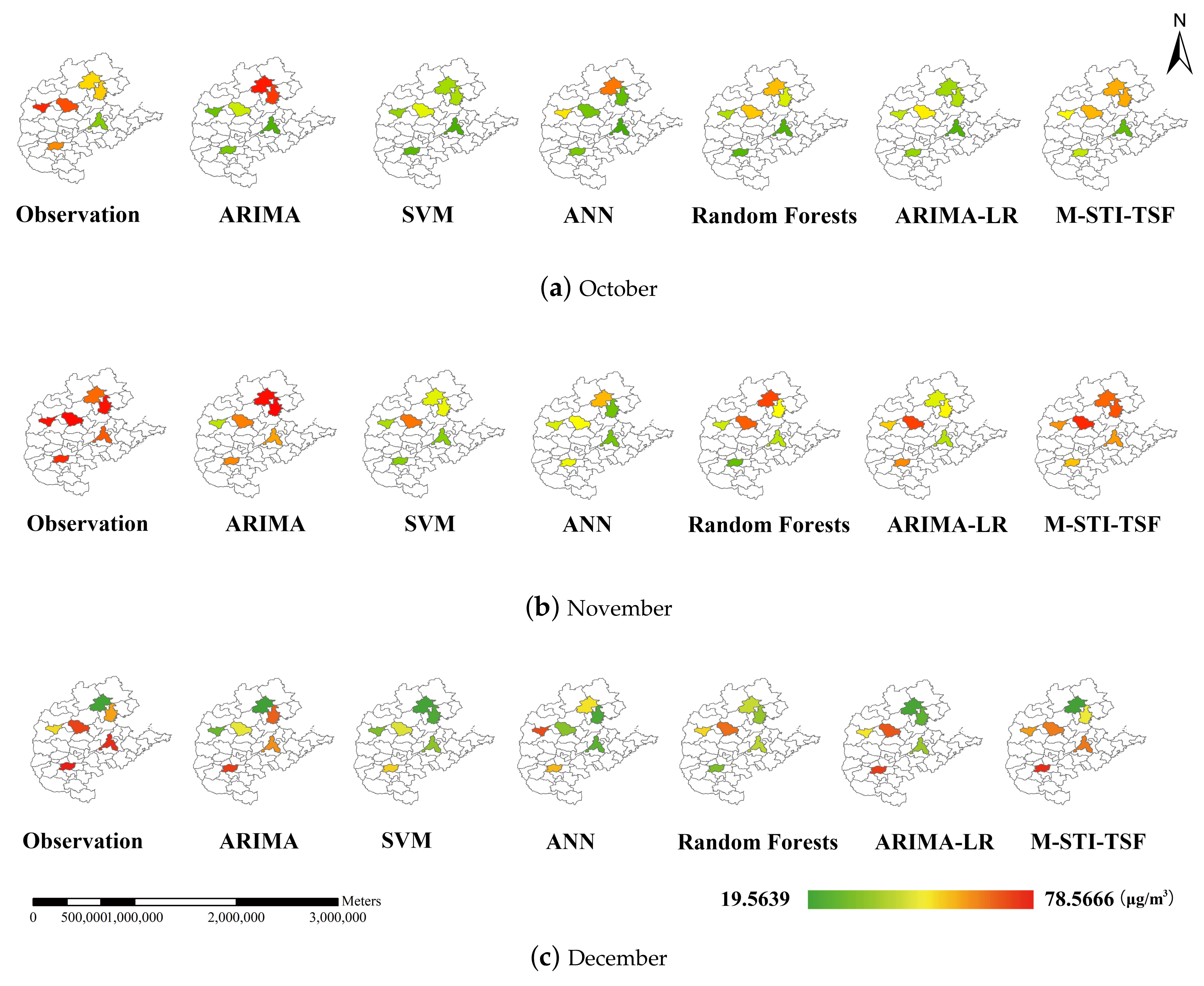
This section focuses on analysing the prediction results of traditional models and the M-STI-TSF model. From the experimental results shown in Figure 4, the prediction curves generated by the M-STI-TSF model are closer to the observed values and follow most of the upward and downward trends. It can be ensured that the proposed model offers better generalization ability over other benchmark models, which also verifies that the short-term trend information extracted by the tracking-differentiator method can enhance the precision of time series forecasts. These significant prediction accuracy improvements benefit from tracking-differentiator technology, short-term trend information, and a reasonable hybrid prediction system architecture. Especially when traditional methods produce large errors in one or more data sets in multiple experiments, we can find that the M-STI-TSF model can still maintain a good generalization ability, which also proves that the new model has strong robustness. Note that due to the use of short-term trend information, the M-STI-TSF model is more effective in tracking abrupt changes in PM 2.5 concentrations when there are large fluctuations. The theoretical basis for this is the tracking-differentiator’s insensitivity to noise and good tracking ability to signals. Short-term trend information makes up for the lack of understanding of the short-term development direction of time series in traditional models. In addition, from the statistical results in Table 2, it is clear that the MAE and RMSE of the M-STI-TSF model are significantly smaller than traditional models. For example, the MAE of the M-STI-TSF model at the Beijing site has decreased by 17.65%, 6.01%, 18.34%, and 15.19% compared to the ARIMA, SVM, ANN and Random Forests models, respectively. Similar conclusions can also be intuitively demonstrated in other research sites, showing that the proposed method has the smallest MAE and RMSE. This evidence proves that the M-STI-TSF model may be more appropriate for such a time series prediction issue consisting of PM 2.5 concentrations with cumulative effects. However, it is worth noting that the ARIMA model can better track fluctuations in the Beijing and Tianjin dataset as observed in Figure 4, possibly due to the distribution characteristics of different data sets. In addition, ARIMA exhibits the strongest R correlation between the predicted results and the true values in the Beijing and Tianjin data sets, which is consistent with ARIMA’s own linear characteristics. The simulation experiment aims to minimize the MAE indicator, so the M-STI-TSF model is not superior to traditional models for a certain indicator value, especially for indicator R. This is because R describes the linear correlation between the predicted results and the true values, and cannot accurately reflect the true intrinsic non-linear relationship. Overall, for multiple evaluation indicators, the M-STI-TSF model has the best comprehensive evaluation. Although the MAE and RMSE of the ANN and RF models at the Taiyuan site are acceptable, the correlation between the predictive results and the observed values may not be linearly expressed when the R value is small. The reason why multiple evaluation indexes are used is to comprehensively verify that a prediction model incorporating short-term trend information can achieve stable improvement in prediction performance. Figure 5 shows the comparison between the predicted results of various prediction models and observed values in October, November and December, where the color change from green to red represents a gradually increasing monthly average concentration. The prediction results of the M-STI-TSF model in the figure are closest to the observed values, especially the most significant in November. Meanwhile, the prediction results of ANN and SVM show a state of being lower than the true value. The M-STI-TSF model integrates short-term trend information to improve the ability to predict the direction of time series development, which exhibits better generalization ability than traditional prediction models.

4.3. Comparison of Prediction Results between M-STI-TSF Model and Hybrid Model ARIMA-LR

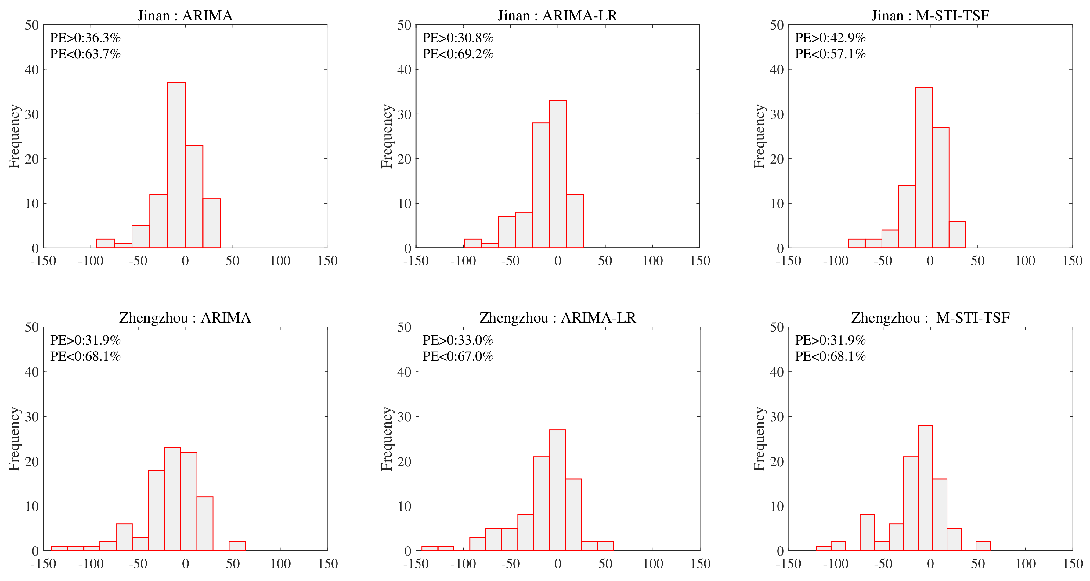
In order to further verify that the good generalization ability of the M-STI-TSF model comes from short-term trend information rather than the hybrid system construction method, this section mainly compares and analyses the M-STI-TSF and ARIMA-LR models based on the similar hybrid system construction principle. The core idea of the ARIMA-LR model is to predict different input feature sequences using the ARIMA method, and then fit these prediction results using a linear regression algorithm to estimate the final PM 2.5 forecasting results. The main difference between these two hybrid models is whether short-term trend information extracted by the differentiator is used. Figure 6 shows the boxplot composed of the observed values and the predicted results of ARIMA, ARIMA-LR, and M-STI-TSF models. The upper and lower quartiles form the upper and lower sides of the box, and the median of the data is represented by horizontal lines located within the box. The whiskers extending from the bottom and top of the box represent the minimum and maximum non-outliers. As shown in the figure, for all research sites, there is a remarkable difference in the data distribution between predicted and observed values, which is due to the strong uncertainty of PM 2.5 daily concentration influenced by various factors, such as meteorological factors, terrain factors, and emission sources, etc. However, the prediction results of the M-STI-TSF model are still the closest to the distribution of observed values compared to other prediction systems. Especially, the whisker extension range predicted by the M-STI-TSF model is smaller than that of the observed values, which means that there is a large error in the tracking of the non-outliers with the minimum or maximum value, although the M-STI-TSF model performs best in other data sets, except for the Beijing and Tianjin data sets. Short-term trend information plays a role in tracking data with large fluctuations, but it is undeniable that the relevant prior knowledge should be further integrated to improve the prediction performance of minimum and maximum non-outliers. The frequency distribution of prediction errors (PE) for prediction models of each site calculated during the testing period is shown in Figure 7. The M-STI-TSF model exhibits a relatively balanced state with respect to the number of PE < 0 and PE > 0 on datasets except for Tianjin and Zhengzhou. That is to say, the proposed model enhances the prediction accuracy identified by the index MAE, but the large range of test data in Tianjin and Zhengzhou still remains underestimated. It is worth noting that the prediction errors of the M-STI-TSF model are more concentrated at 0, which means that the larger errors generated by the traditional models have been corrected. The above analysis shows that the M-STI-TSF model has improved both in terms of prediction performance and distribution of prediction results. In particular, by comparing the prediction results of ARIMA and ARIMA-LR models, it is found that the idea of hybrid model construction is helpful to improve the generalization ability. This view has also been proved by [20,21], because the hybrid model reflects the advantages of multiple models, and avoids the over-sensitivity of a single model to data and the limitations of the model itself. Therefore, it can be considered that the excellent generalization ability of the M-STI-TSF model lies not only in the idea of hybrid models, but also in the application of short-term trend information.

5. Discussion

The experimental results show that the M-STI-TSF model proposed in this paper effectively improves the stability and generalization ability of the prediction model due to the introduction of short-term trend information. However, there are still some details worth further discussion during the construction process of the prediction system.
(1) In our research, we represent short-term trend information in differential form. Because EDD shows good noise insensitivity, it is used to extract short-term trend information. However, it cannot be excluded that there are more suitable tracking-differentiator, which is worthy of further study. (2) The solution of the multivariable input problem in the prediction system uses linear regression, which improves the comprehensiveness of input information and implies the linear intrinsic relationship between input features and outputs. The nonlinear relationship between input and output needs to be further validated using nonlinear models.

6. Conclusions

The cumulative effect of PM 2.5 concentration brings strong correlation between adjacent data in time series, manifested as short-term trend characteristics, which is appropriately utilized to supplement the statistical information of traditional prediction systems and expand modeling information, resulting in effective improvement of the model’s prediction ability. Based on the characteristics of dynamic systems, this article proposes the use of EDD to decompose and reconstruct the original signal, which realizes one-dimensional time series prediction including short-term trend information represented by differentiation. Furthermore, linear regression completes the fitting of multiple one-dimensional variable prediction results, making it possible to construct a dynamic prediction system with multi-dimensional inputs. The simulation experiments of PM 2.5 daily concentration prediction in six cities in North China have verified that short-term trend information can effectively improve the model’s generalization ability.
Therefore, we can draw the following conclusions: (1) It is feasible to use tracking-differentiator to extract short-term trend information. (2) Short-term trend information can help improve the accuracy of PM 2.5 concentration prediction, which can be extended to other implicit short-term trend information time series. (3) The STI-TSF model, which integrates short-term trend information extracted by EDD, has completed the one-dimensional time series prediction task and implemented a dynamic prediction system architecture. (4) The M-STI-TSF model solves the high-dimensional input problem of prediction systems, making it more suitable for real-world prediction problems with multivariate inputs.

Author Contributions

Conceptualization and methodology, P.W.; editing and writing of draft, X.H.; visualization and supervision, H.F.; data curation and software, G.Z. All authors have read and agreed to the published version of the manuscript.

Funding

This work is funded by the National Social Science Fund of China (No. 20BTJ045).

Institutional Review Board Statement

Not applicable.

Informed Consent Statement

Not applicable.

Data Availability Statement

This data can be found here: [http://www.tianqihoubao.com/] (accessed on 1 April 2023).

Conflicts of Interest

The authors declare no conflict of interest.

References

  1. Cheng, F.Y.; Feng, C.Y.; Yang, Z.M.; Hsu, C.H.; Chan, K.W.; Lee, C.Y.; Chang, S.C. Evaluation of real-time PM2.5 forecasts with the WRF-CMAQ modeling system and weather-pattern-dependent bias-adjusted PM2.5 forecasts in Taiwan. Atmos. Environ. 2021, 244, 117909. [Google Scholar] [CrossRef]
  2. Jin, X.; Cai, X.; Yu, M.; Song, Y.; Wang, X.; Kang, L.; Zhang, H. Diagnostic analysis of wintertime PM2.5 pollution in the North China Plain: The impacts of regional transport and atmospheric boundary layer variation. Atmos. Environ. 2020, 224, 117346. [Google Scholar] [CrossRef]
  3. Yan, D.; Lei, Y.; Shi, Y.; Zhu, Q.; Li, L.; Zhang, Z. Evolution of the spatiotemporal pattern of PM2.5 concentrations in China—A case study from the Beijing-Tianjin-Hebei region. Atmos. Environ. 2018, 183, 225–233. [Google Scholar] [CrossRef]
  4. Zhou, Y.; Chang, F.J.; Chang, L.C.; Kao, I.F.; Wang, Y.S.; Kang, C.C. Multi-output support vector machine for regional multi-step-ahead PM2.5 forecasting. Sci. Total Environ. 2019, 651, 230–240. [Google Scholar] [CrossRef] [PubMed]
  5. Kow, P.Y.; Wang, Y.S.; Zhou, Y.; Kao, I.F.; Issermann, M.; Chang, L.C.; Chang, F.J. Seamless integration of convolutional and back-propagation neural networks for regional multi-step-ahead PM2.5 forecasting. J. Clean. Prod. 2020, 261, 121285. [Google Scholar] [CrossRef]
  6. Yeo, I.; Choi, Y.; Lops, Y.; Sayeed, A. Efficient PM2.5 forecasting using geographical correlation based on integrated deep learning algorithms. Neural Comput. Appl. 2021, 33, 15073–15089. [Google Scholar] [CrossRef]
  7. Samal, K.K.R.; Babu, K.S.; Das, S.K. Multi-directional temporal convolutional artificial neural network for PM2.5 forecasting with missing values: A deep learning approach. Urban Clim. 2021, 36, 100800. [Google Scholar] [CrossRef]
  8. Zhou, Y.; Chang, L.C.; Chang, F.J. Explore a Multivariate Bayesian Uncertainty Processor driven by artificial neural networks for probabilistic PM2.5 forecasting. Sci. Total Environ. 2020, 711, 134792. [Google Scholar] [CrossRef] [PubMed]
  9. He, H.; Gao, S.; Jin, T.; Sato, S.; Zhang, X. A seasonal-trend decomposition-based dendritic neuron model for financial time series prediction. Appl. Soft Comput. 2021, 108, 107488. [Google Scholar] [CrossRef]
  10. Zhou, C.; Chen, X. Predicting energy consumption: A multiple decomposition-ensemble approach. Energy 2019, 189, 116045. [Google Scholar] [CrossRef]
  11. Zhou, C.; Chen, X. Predicting China’s energy consumption: Combining machine learning with three-layer decomposition approach. Energy Rep. 2021, 7, 5086–5099. [Google Scholar] [CrossRef]
  12. Bas, M.; Ortiz, J.; Ballesteros, L.; Martorell, S. Analysis of the influence of solar activity and atmospheric factors on 7Be air concentration by seasonal-trend decomposition. Atmos. Environ. 2016, 145, 147–157. [Google Scholar] [CrossRef]
  13. Song, Z.; Fu, D.; Zhang, X.; Han, X.; Song, J.; Zhang, J.; Wang, J.; Xia, X. MODIS AOD sampling rate and its effect on PM2.5 estimation in North China. Atmos. Environ. 2019, 209, 14–22. [Google Scholar] [CrossRef]
  14. Xu, W.; Wu, Q.; Liu, X.; Tang, A.; Dore, A.J.; Heal, M.R. Characteristics of ammonia, acid gases, and PM2.5 for three typical land-use types in the North China Plain. Environ. Sci. Pollut. Res. 2016, 23, 1158–1172. [Google Scholar] [CrossRef] [PubMed]
  15. Huang, K.; Xiao, Q.; Meng, X.; Geng, G.; Wang, Y.; Lyapustin, A.; Gu, D.; Liu, Y. Predicting monthly high-resolution PM2.5 concentrations with random forest model in the North China Plain. Environ. Pollut. 2018, 242, 675–683. [Google Scholar] [CrossRef] [PubMed]
  16. China National Environmental Monitoring Center. Air Quality Status Report; China National Environmental Monitoring Center: Beijing, China, 2021. [Google Scholar]
  17. Feng, H.; Qian, Y. A Linear Differentiator Based on the Extended Dynamics Approach. IEEE Trans. Autom. Control 2022, 67, 6962–6967. [Google Scholar] [CrossRef]
  18. Feng, H.; Guo, B.Z. Extended dynamics observer for linear systems with disturbance. Eur. J. Control 2023, 71, 100806. [Google Scholar] [CrossRef]
  19. Wang, Z.; Li, J.; Liang, L. Spatio-temporal evolution of ozone pollution and its influencing factors in the Beijing-Tianjin-Hebei Urban Agglomeration. Environ. Pollut. 2020, 256, 113419. [Google Scholar] [CrossRef] [PubMed]
  20. Ordóñez, C.; Sánchez Lasheras, F.; Roca-Pardiñas, J.; de Cos Juez, F.J. A hybrid ARIMA–SVM model for the study of the remaining useful life of aircraft engines. J. Comput. Appl. Math. 2019, 346, 184–191. [Google Scholar] [CrossRef]
  21. Khashei, M.; Bijari, M. A novel hybridization of artificial neural networks and ARIMA models for time series forecasting. Appl. Soft Comput. 2011, 11, 2664–2675. [Google Scholar] [CrossRef]
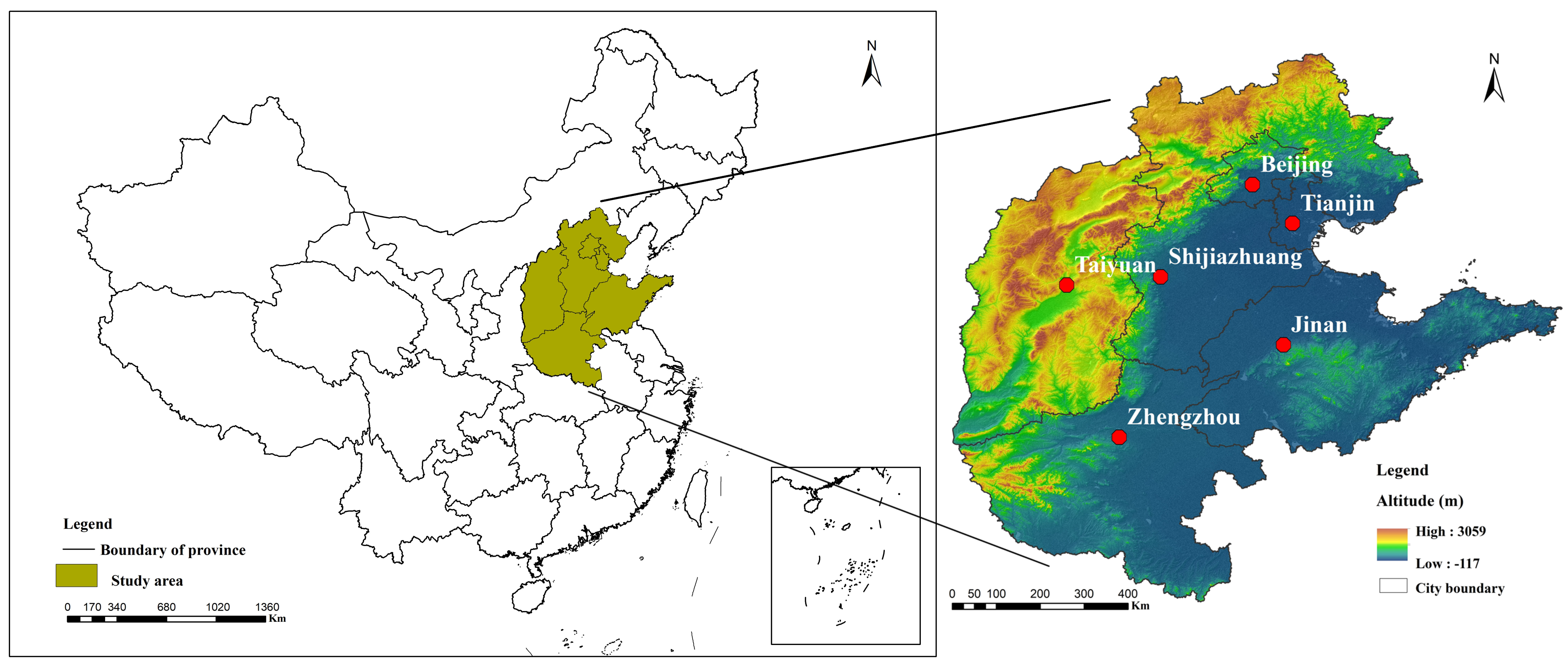
Figure 1. Physical geography of the study area.
Sustainability 15 16264 g001
Figure 2. Prediction results of STI-TSF model for air pollutant concentration.
Sustainability 15 16264 g002
Figure 3. M-STI-TSF modeling process.
Sustainability 15 16264 g003
Figure 4. Prediction results of M-STI-TSF model and traditional models for PM 2.5 concentration.
Sustainability 15 16264 g004
Figure 5. Prediction results of PM 2.5 monthly average concentration.
Sustainability 15 16264 g005
Figure 6. Prediction results of M-STI-TSF model and ARIMA-LR model for air pollutant concentration.
Sustainability 15 16264 g006aSustainability 15 16264 g006b
Figure 7. Prediction results of M-STI-TSF model and ARIMA-LR model for air pollutant concentration.
Sustainability 15 16264 g007aSustainability 15 16264 g007b
Table 1. Calculation results of mutual information between PM 2.5 and historical concentration of pollutants.
Monitoring SitePM 2.5 PM 10 SO 2 NO 2 COO 3
Beijing3.47174.05690.43982.92850.17924.1748
Tianjin3.74964.29471.46253.41320.26874.3273
Shijiazhuang4.07274.68671.84963.53790.38774.5385
Taiyuan4.02594.70172.26993.54980.43494.3875
Jinan3.74034.31942.11403.34830.41164.4225
Zhengzhou4.11334.69491.73823.26160.41114.5803
Table 2. Prediction accuracy of the prediction models on the test set.
IndexModelBeijingTianjinShijiazhuangTaiyuanJinanZhengzhou
MAE ( μ g/m 3 )ARIMA22.976624.971922.933924.043716.999725.2036
SVM20.131223.273121.538723.033618.520129.2287
ANN23.170925.088225.165223.502220.749527.3979
Random Forests22.309624.285821.276422.820619.529831.6621
ARIMA-LR20.655623.535820.996521.297118.292725.2138
M-STI-TSF18.920220.610819.185719.926315.500323.4288
RMSE ( μ g/m 3 )ARIMA37.959835.284931.445432.517824.131537.4335
SVM27.605131.423528.726031.668126.262742.1796
ANN31.157334.787233.787932.389427.980941.0037
Random Forests30.142433.998530.070931.566527.255148.1769
ARIMA-LR28.224932.037027.279129.468826.406137.9620
M-STI-TSF26.801727.503425.431526.703421.885534.6578
RARIMA0.78410.79710.70950.56720.63030.6668
SVM0.57500.65920.73750.60270.68930.7183
ANN0.44930.60460.68660.12490.65680.7046
Random Forests0.49510.50290.61460.28430.54650.5484
ARIMA-LR0.55280.64400.68250.55250.68820.6834
M-STI-TSF0.59670.69240.75670.61190.70640.7224
Disclaimer/Publisher’s Note: The statements, opinions and data contained in all publications are solely those of the individual author(s) and contributor(s) and not of MDPI and/or the editor(s). MDPI and/or the editor(s) disclaim responsibility for any injury to people or property resulting from any ideas, methods, instructions or products referred to in the content.