Spatial–Temporal Evolution and Driving Factors of China’s High-Quality Economic Development

Abstract

Combining an indicator system developed based on existence–relatedness–growth (ERG) needs and multiple weighting approaches, this paper evaluates the level of high-quality economic development (HQED) in Chinese provinces from the perspective of human well-being from 2007 to 2020. Spatial analysis, Dagum’s Gini coefficient (DGC), and spatial econometric modeling were employed to investigate the spatial–temporal evolutionary characteristics, regional differentiation, and driving factors of HQED in China. The following conclusions are drawn: (1) During the period of 2007–2019, the level of Chinese HQED showed a stable upward trend, and gradually produced the development characteristics of “only super power and multi-great power” and spatial features of “point, line and plane”, with Beijing as the absolute leader, the southeastern coastal region as the advantageous belt, and the relatively advantageous plane in central and western areas with Shaanxi as the core. (2) The degree of spatial differentiation in Chinese provincial HQED narrowed year by year, with intra-regional differentiation organized as follows: eastern > northeastern > western > central; inter-regional differentiation was concentrated in the development gaps across the other three major regions and the eastern areas. (3) Chinese provincial HQED had a significant spatial autocorrelation characteristic, which was further revealed by the spatial Durbin model (SDM) to be a siphon effect at the national and regional levels, i.e., the plundering of the resources and development opportunities of weaker provinces by stronger ones. (4) Driving factors such as economic scale, urbanization level, resource endowment, government size, green technological innovation, industrial structure upgrading, and environmental regulations affected HQED at the national level and in the four major regions to varying degrees. These findings could contribute to policymakers’ efforts to design targeted regional development policies during the transition period of China’s economic development.

1. Introduction

China has achieved extensive and renowned economic growth following the program of reform and opening-up [1]. However, with the fading of traditional advantages (i.e., factor, structural, and institutional dividends) and the disappearance of latecomer advantages (i.e., urbanization and globalization), China’s GDP growth rate basically stabilized below 8% after 2012. Furthermore, the realization of the second centennial goals is seriously constrained by the difficulties of cutting-edge science and technology strangleholds, uncoordinated regional development, increasing ecological and environmental constraints, elevated geopolitical risks, and widening income distribution gaps [2]. Given the fundamental change in the primary social inconsistencies and the stage-specific characteristics of economic development in the contemporary era, the 19th Communist Party Congress has made the important assertion that the period of high-speed growth has given way to a period of high-quality development of the Chinese economy. High-quality economic development (HQED) has thus become the new proposition of the era and a hot research topic in China [3].

Quantitative expansion and qualitative improvement are the two core issues of economic growth. Long-term economic theory and practice have often paid more attention to the former. However, as societies have paid high socio-economic, resource-related, and environmental costs for development, academics have begun to question the proposition that economic growth inevitably improves welfare [4]. In contrast, the quality of economic growth is undoubtedly richer in both connotation and extension, a fact that has attracted extensive attention from researchers in various fields. Kamaev [5], who first proposed the definition, suggested that the quality of economic growth is more adequately conveyed by assessing the satisfaction of people’s needs than emphasizing the growth of material wealth, but that the two tasks should not be regarded in opposition to each other. With the accumulation of research, the interpretation of the quality of economic growth has been gradually deepened: according to classical economic theory, the high quality of an economy can be viewed as a consequence of the national economic system reaching a state of dynamic equilibrium between aggregate supply and demand, which relies on the two-way interaction of expansion on a market scale and the deepening of labor division, as well as the organic combination of supply-side structural reforms and the expansion of domestic demand [6]. Welfare economics pays particular attention to the well-being improvements that economic development brings to the population at a given moment, as well as its future sustainability [7]. Mai et al. [8] emphasized that welfare improvements need to be supported by a favorable policy environment and economic strength, which is the key to the high well-being indices in Beijing and Guangdong. The integrated perspective, following the views of Barrow [9] and Thomas et al. [10], further summarize the quality of economic growth as a combination of factors such as equal educational opportunities, ecological optimization, improved market mechanisms, efficient resource allocation, and optimized economic structure [11]. From a multi-dimensional perspective, the enhancement of the quality of economic growth is represented by an improvement in the quality of products and services at the microlevel [12], the upgrading of industrial structure and the alleviation of regional development inequity at the mesolevel [13], and a reduction in energy consumption and an improvement in economic performance at the macrolevel [14].

From the perspective of HQED-level evaluation, existing research can be broadly categorized into two types. In order to simplify their analyses, a few researchers have used single indicator measures such as per capita income, real per capita GDP, the Gini coefficient, the size of the population in poverty, ecological footprint, satellite image data, and total factor productivity [3,15,16,17,18]. For instance, Liu et al. [19] used resource inputs (labor, capital, and energy), desired outputs (GDP), and undesired outputs (industrial wastewater, sulfur dioxide, and soot) to calculate green total factor productivity for the purpose of measuring the level of HQED. While the selection of a single indicator metric has benefits, it tends to capture only one aspect of economic, social, and ecological benefits, potentially leading to incomplete measurements [20]. Precisely for this reason, more researchers prefer to examine HQED from a multi-dimensional perspective, such as the human development index (HDI) [21], the sustainable development index (SDI) [22], gross national happiness (GNH) [23], and comprehensive measurement using the new development philosophy of innovation, coordination, greenness, openness, and sharing [24]. Based on the new development philosophy, for example, Li et al. [25] and Chen and Huo [26] revealed the stable growth characteristics of HQED levels in China at different spatial scales.

Moreover, researchers have further revealed the impact of key issues in the transition development stage on HQED. Some have found that industrial agglomeration, the digital economy, and two-way FDI play facilitating roles to varying degrees [2,24,27] and that resource misallocation, pollution, and population aging exert restraining effects [28,29,30], while factors like environmental regulation and economic growth targets [19,31] may vary in effect over time and space.

Researchers have made useful attempts to elucidate the connotation and extension of HQED, as well as to explore its level and influencing factors, but the following aspects remain in need of further exploration. First, academics and Chinese authorities generally agree that HQED is a model of economic development in the new era with the fundamental goal of satisfying the population’s growing need for a better life [25], although no universal definition has yet been developed. However, from the literature available to us, the research into HQED under this goal framework is inadequate. Second, in studies of multi-indicator comprehensive evaluations of HQED, researchers tend to use a single weight assignment method such as an entropy technique [2,13] or principal component analysis [31]. However, it is difficult to guarantee the robustness of results obtained using single methods. Third, the majority of research uses the ordinary least-squares (OLS) approach to identify the variables that affect HQED. Unfortunately, this method may further lead to biased estimation, as it cannot address the difficulties caused by spatial factors.

Given these limitations, this manuscript attempts to make the following marginal contributions. First, based on the index system established by the hierarchy of needs theory, we evaluate the HQED level of Chinese provinces from the perspective of the ultimate goal of economic development, contributing to the improvement of the micro-foundation of HQED evaluation and enriching the existing literature. Second, we adopt the weight assignment methods of subjective, objective, and subjective–objective combinations to guarantee the credibility of the measurement results. Third, we employ spatial visualization methods and the Dagum’s Gini coefficient (DGC) to portray regional inequality in HQED, which may assist policymakers in designing differentiated regional development strategies. Fourth, an interesting finding, which requires the attention of authorities, is that the spatial impacts of HQED at different levels all manifest as a siphoning effect, i.e., developed provinces deprive lagging regions of resources and development opportunities.

The remainder of this manuscript is organized as follows. The research methodologies and data sources are discussed in the subsequent section. Section 3 reveals and analyzes the features of spatial–temporal evolution and regional inequality of HQED in China, with Section 4 further emphasizing the driving factors via spatial econometric modeling. The last section summarizes the conclusions of the study and provides policy implications.

2. Materials and Methods

2.1. Data Sources and Pre-Processing

This paper applies a study period of 2007–2020, and a study area of 30 provinces’ administrative regions in China, except for Taiwan, Macao, Hong Kong, and Tibet, where data are severely limited. The data are primarily taken from the corresponding years of China Statistical Yearbook, the National Bureau of Statistics of China (http://www.stats.gov.cn/) (accessed on 10 October 2023), Washington University in St. Louis (https://wustl.edu/) (accessed on 25 August 2023), and the Standard Map Service website (http://bzdt.ch.mnr.gov.cn/) (accessed on 2 September 2023).

In order to mitigate the effect of pricing elements, the corresponding indicators are converted and deflated using the average exchange rates, the GDP index, and the price indices for consumption, housing, retail sales of goods, imported and exported goods, and transportation and communication, with the year 2000 serving as the base period. Moreover, we logarithmize the relevant variables in the regression process to weaken covariance and avoid heteroskedasticity.

2.2. Evaluation of HQED

2.2.1. Indicator System

The ultimate goal of economic production is to satisfy the actual needs of the people [5]. Conversely, the degree of satisfaction of needs reflects the level and quality of economic development [32]. Therefore, we aim to construct a goal-oriented HQED evaluation index system. In contrast to the previous stage of high-speed and rough development, residents now expect not only adequate food and clothing, but also greater access to schooling, more secure employment, adequate incomes, more dependable social security, higher standards of health and medical care, more comfortable housing, beautiful environments, broader spiritual engagement and cultural scenes, and that their children also see improved standards.

In order to effectively reflect the degree of satisfaction of residents’ needs, we followed the existence–relatedness–growth (ERG) needs theory of Alderfer [33]. It is proposed on the basis of Maslow’s needs, avoiding the assumption of a strict progressive relationship between the layers of needs (i.e., higher-level wants only arise after lower-level wants have been satisfied), effectively solving the problem of blurred boundaries. This renders the technique more relevant to the present scenario. Referring to Schneider and Alderfer [34], and Yang et al. [35], all physical and physiological needs are considered existence needs. Under the premise of limited resources and unlimited wants [36], what an individual gains is another’s loss. This implies that the more one gains under the same conditions, the more one’s existence needs can be satisfied. The satisfaction of relatedness needs depends on the process of sharing and interacting with others, which is significantly different from existence needs and reflects the social nature of human beings. Growth needs include the individual’s need to have a creative or productive impact on oneself and the environment, and its satisfaction depends on whether the individual can find the opportunity to give full play to their potential. For quantitative analysis, it is necessary to refine ERG needs and further set measurement indicators. Drawing on the principles of the HDI, the SDI, and the GNH [21,22,23], the satisfaction of existence needs is portrayed in terms of basic living conditions, medical and health conditions, and public safety and security; the satisfaction of relatedness needs is measured in terms of the sense of belonging and tolerance, convenience, and openness that the district provides to the residents; and the satisfaction of growth needs is reflected by the self-development ability of individuals and the support provided by society.

Table 1. The indicator system of HQED from 2007 to 2020 in China.

ERG Needs	Criterion Layer	Indicator Layer	Calculation Method	Attributes
Existence needs	Basic living conditions	Revenue growth elasticity	Per capita disposable income growth rate/GDP growth rate	+
		Poverty incidence	Number of minimum subsistence allowances/resident population number	−
		Engel coefficient	Engel coefficient	−
		Water penetration rate	Water penetration rate	+
		Housing condition	Average sales price of commercial houses/per capita disposable income	−
	Medical and health conditions	Health staffing ratio	Number of staff in medical facilities/resident population number	+
		Health bed ratio	Number of beds in medical facilities/resident population number	+
		Health awareness	Number of health check-ups/resident population number	+
	Public safety and security	Social security	Crime rate	−
		Traffic safety	Traffic accident rate	−
		Eco-safety	PM2.5 concentration	−
		Emergency management capability	Public security financial expenditure/local financial general budget expenditure	+
Relatedness needs	Sense of belonging and tolerance	Family harmony	Crude divorce rate	−
		Labor security	Number of workers’ compensation insurance participants/ employed population number	+
		Social interaction	Number of social organization units/resident population number	+
		Leisure space	Park green space area/resident population number	+
		Demand structure	Gross retail sales of social consumer goods/GDP	+
		Urban and rural structure	Per capita disposable income of urban residents/per capita disposable income of rural residents	−
	Convenience and openness	Place attachment	Resident population number/registered population number	+
		Road network construction	Per capita road space in urban area	+
		Internet construction	Number of internet users/resident population number	+
		Construction for telecoms and post	Total postal and telecommunication services/resident population number	+
		Convenient details construction	Public toilets of more than three types per 10,000 people	+
		Tourism attraction	Number of international tourists received	+
		Foreign connection	Total import and export of goods/GDP	+
Growth needs	Self-development	Human capital	Average education years (year sets: elementary school: 6; middle school: 9; high school: 12; college: 15; undergraduate: 16; graduate: 19)	+
		Realization of personal values	Urban registered unemployment rate	−
		Consumption expectations	Consumption expenditure per capita/per capita disposable income	+
		Spiritual and cultural needs	Number of books on loan/resident population number	+
		Parenting stress	Total dependency ratio (non-working-age population number/working-age population number)	−
	Social support	Investment-based public expenditure	Education, science and technology, culture, sports and media, social security, and employment financial expenditure/local financial general budget expenditure	+
		R&D investment intensity	Internal expenditure on R&D/GDP	+
		Activity of technology trading	Technology transaction volume/GDP	+
		Economic growth fluctuation	Economic growth rate variability during the last five years	−
		Energy consumption elasticity	Growth rate for energy use/GDP growth rate	−

displays the HQED indication system for China.

2.2.2. Evaluation Methods

We employed subjective and objective measures, as well as a mix thereof, to assign weights for the purpose of assuring the accuracy of the evaluation findings. Among them, the subjective technique was used to assign the same weight to each indicator, which is not described here. The objective strategies comprised the entropy method and the improved criteria importance through intercriteria correlation (I-CRITIC) approach. Additionally, the combined techniques, including I and II, were synthetic methods. According to the attributes, we standardized the positive and negative indices using Equations (1) and (2), respectively:

$$x_{ij}=\frac{X_{ij}-\min \left(X_j\right)}{\max \left(X_j\right)-\min \left(X_j\right)}$$

(1)

$$x_{ij}=\frac{\max \left(X_j\right)-X_{ij}}{\max \left(X_j\right)-\min \left(X_j\right)}$$

(2)

where x_ij represents the standardized indicator value, X_ij stands for the initial value of j indicators in i provinces, and minX and maxX refer to the minimum and maximum values, respectively.

• Entropy method. This technique defines each indicator’s significance in relation to the level of variability [2]. Indicators with lower information entropy convey more information and weight; conversely, indicator weight will be lighter. Specifically, after the standardization process, normalization is performed according to Equation (3), the coefficient of variation is calculated utilizing Equation (4), and then, Equations (5) and (6) are employed to determine the indicator weights and calculate the composite score.

$$p_{ij}=\frac{x_{ij}}{{\displaystyle \sum {}_{i=1}^m}}$$

(3)

$$d_j=1+\frac{1}{\ln m}{\displaystyle \sum _{i=1}^m{p}_{ij}}\ln p_{ij}$$

(4)

$$w{e}_j=\frac{d_j}{{\displaystyle {\sum }_{j=1}^m{d}_j}}$$

(5)

$$HQE{D}_E={\displaystyle \sum _{j=1}^{m}w{e}_j{p}_{ij}}$$

(6)

In the above equations, d_j indicates the variance coefficient of index j, we_j refers to the weight of indicator j, and HQED_E represents the composite score of each province by the entropy method.

• I-CRITIC method. This method, which is also an objective technique, measures the weight of an indicator by evaluating its volatility and conflict. The standard deviation and correlation coefficient are employed to describe volatility and conflict, respectively [37]. Previous studies have found that the standard deviation carries dimension; the correlation coefficient may be negative, but essentially, conflictedness is only related to the absolute magnitude of the correlation coefficient. Following Krishnan et al. [38], we improved the CRITIC approach and obtained the I-CRITIC approach: first, the standard deviation is replaced by the standard deviation coefficient of the mean to eliminate the effect of dimension; second, the absolute value is taken for the correlation coefficient to eliminate the effect of positive and negative signs. Therefore, Equations (7) and (8) reflect the information content and weight of the indicators, respectively, and Equation (9) expresses the composite score.

$$c_j=\frac{{\sigma }_j}{{\overline{x}}_j}\cdot {\displaystyle \sum _{k=1}^n\left(1-\left|r_{jk}\right|\right)}$$

(7)

$$wi{c}_j=\raisebox{1ex}{$c_j$}\!\left/ \!\raisebox{-1ex}{${\displaystyle \sum _{j=1}^m{c}_j}$}\right.$$

(8)

$$HQE{D}_{IC}={\displaystyle \sum _{j=1}^{m}wi{c}_j{x}_{ij}}$$

(9)

In the above equations, σ and $\overline{x}$ stand for the standard deviation and mean of index j, and r_jk indicates the correlation coefficient for indices j and k.

Combinations I and II. These techniques incorporate the entropy and I-CRITIC strategies in combination, as well as the researcher’s personal assessment. Without adding additional conditions, Combination I is obtained as follows:

$$w{c}_{\mathrm{I}}=\beta w{e}_j+\left(1-\beta \right)wi{c}_j$$

(10)

where β = 0.5, with both methods considered equally important. The calculation of the composite score is basically the same as Equation (9) and will not be repeated.

According to ERG theory, we consider existence, relatedness, and growth needs to be equally important to individuals. Therefore, Combination II first assigns the same weight, i.e., 1/3, to each need layer, and then, synthesizes the entropy weight and I-CRITIC methods. The composite score obtained from Combination II, which better reflects the combination of subjectivity and objectivity, is calculated as follows:

$$\begin{array}{l}HQE{D}_{\mathrm{II}}=HQE{D}_E+HQE{D}_R+HQE{D}_G\\ =\left[{\displaystyle \sum _{j=1}^{12}\frac{\beta w{e}_{Ej}+\left(1-\beta \right)wi{c}_{Ej}}{3}}+{\displaystyle \sum _{j=1}^{13}\frac{\beta w{e}_{Rj}+\left(1-\beta \right)wi{c}_{Rj}}{3}}+{\displaystyle \sum _{j=1}^{10}\frac{\beta w{e}_{Gj}+\left(1-\beta \right)wi{c}_{Gj}}{3}}\right]\cdot x_{ij}\end{array}$$

(11)

where subscripts E, R, and G denote the three need layers, respectively.

2.3. DGC

With the help of the ArcGIS 10.2 platform, Origin 2021 software, and DGC, we reveal the spatial–temporal evolution characteristics of and regional differences in HQED in Chinese provinces. The latter is highlighted here. DGC [39], which can more effectively address the cause of geographical differentiation and the difficulties in regional overlap than the Thiel index and the traditional Gini coefficient, is frequently used to identify regional resource allocation and development inequalities [40]. The general formula for DGC is as follows:

$$G=\frac{{\displaystyle \sum _{j=1}^k}{\displaystyle \sum _{h=1}^k}{\displaystyle \sum _{i=1}^{n_j}}{\displaystyle \sum _{r=1}^{n_k}}\left|y_{ji}-y_{hr}\right|}{2n^2\overline{y}}$$

(12)

where y_ji (y_hr) denotes a province’s HQED level within region j(h), $\overline{y}$ represents the provincial mean of the level of HQED, k and n refer to the number of regions and provinces, and n_j (n_h) stands for the number of provinces within region j(h). Further, G consists of intra-region differences G_w, inter-region differences G_nb, and trans-variance intensity G_t and, meeting G = G_w + G_nb + G_t, is calculated as follows:

$$G_{jj}=\frac{\frac{1}{2{\overline{y}}_j}{\displaystyle {\sum }_{i=1}^{n_j}{\displaystyle {\sum }_{r=1}^{n_j}\left|y_{ji}-y_{jr}\right|}}}{n_j^2}$$

(13)

$$G_{jh}=\frac{{\displaystyle {\sum }_{i=1}^{n_j}{\displaystyle {\sum }_{r=1}^{n_j}\left|y_{ji}-y_{hr}\right|}}}{n_j{n}_h\left({\overline{y}}_j+{\overline{y}}_h\right)}$$

(14)

$$G_w={\displaystyle {\sum }_{j=1}^k{G}_{jj}{p}_j{s}_j}$$

(15)

$$G_{nb}={\displaystyle {\sum }_{j=2}^k{\displaystyle {\sum }_{h=1}^{j-1}{G}_{jh}\left(p_j{s}_h+p_h{s}_j\right)D_{jh}}}$$

(16)

$$G_t={\displaystyle {\sum }_{j=2}^j{\displaystyle {\sum }_{h=1}^{j-1}{G}_{jh}\left(p_j{s}_h+p_h{s}_j\right)\left(1-D_{jh}\right)}}$$

(17)

$$D_{jh}=\frac{d_{jh}-p_{jh}}{d_{jh}+p_{jh}}$$

(18)

$$d_{jh}={\displaystyle {\int }_0^{\infty }d{F}_j(y){\displaystyle {\int }_0^y(y-x)d{F}_h(x)}}$$

(19)

$$p_{jh}={\displaystyle {\int }_0^{\infty }d{F}_h(y){\displaystyle {\int }_0^y(y-x)d{F}_j(y)}}$$

(20)

where G_jj and G_jh stand for the Gini coefficients within province j and between j and h. $p_j=n_j/\overline{y}$ and $s_j=n_j{\overline{y}}_j/n\overline{y}$. d_jh and D_jh represent the differences and relative impacts of HQED between provinces j and h, respectively. p_jh suggests a hypervariable first-order moment, while F(·) is the cumulative distribution function.

2.4. Spatial Econometric Modeling

2.4.1. Model Design

The spatial Durbin model (SDM), developed in the wake of the study of LeSage and Pace [41], is tasked with analyzing the driving factors of HQED in China. The equation is as follows:

$$Y_{jt}=\alpha +\rho \sum _{h=1}^{n}W{Y}_{ht}+\beta X_{jt}+\theta \sum _{h=1}^{n}W{X}_{ht}+{\mu }_j+{\delta }_t+{\epsilon }_{jt}$$

(21)

where Y_jt and X_jt are the explained and explanatory variables in province j in year t, respectively; ρ denotes the coefficient of the spatial lag term of the explained variable; β and θ stand for the regression coefficients and spatial lag term coefficients of the explanatory variables, respectively; W indicates the spatial weight matrix; μ_i and δ_t represent the region- and time-fixed effects, respectively; and α and ε_it indicate the constant and error terms, respectively. For the coefficients ρ and θ, if the estimation result is positive, this indicates that the improvement in a certain index in the developed provinces plays a radiating and driving role for the neighboring provinces, i.e., a spatial spillover effect (or radiation effect); on the contrary, if the estimation result is negative, this implies that the agglomeration advantage of the developed provinces leads to the deprivation of resources and development opportunities for the neighboring lagging provinces, i.e., a siphon effect (or Matthew effect) [42].

2.4.2. Variable Selection

• Explained variable. For the empirical study, the level of HQED in Chinese provinces was picked as the explained variable.
• Explanatory variables. Depending on the connotation of HQED and China’s actual situation in the transition stage, we refer to the literature and select explanatory variables from three aspects: traditional driving factors [1,19], new momentums [27,43], and environmental constraints [30]. Specifically, the traditional drivers include economic scale (PGDP), indicated by per capita GDP; urbanization level (URB), represented by population urbanization rate; resource endowment (RES), computed on the basis of the share of total fixed asset investment that is spent on mining and agriculture; and government scale (GOV), described as the local treasury’s general budget spending in relation to GDP. New momentums include green technological innovation (INN), expressed as the quantity of green invention patents authorized, and upgrades to the industrial structure (IND), as determined by Equation (22). Environmental constraints include command-and-control environmental regulation (ER₁), as obtained in Equation (23), and cost-based environmental regulation (ER₂), expressed in terms of the emission fee, which was changed to an environmental tax after 2018.

$$IN{D}_{jt}=\frac{V_{1jt}\times 1+V_{2jt}\times 2+V_{3jt}\times 3}{GD{P}_{jt}}$$

(22)

$$E{R}_{1jt}=\frac{N_{1jt}+N_{2jt}}{2}$$

(23)

In the above equations, V₁, V₂, and V₃ stand for the primary, secondary, and tertiary industries’ respective added values. N₁ and N₂ are the normalized numbers of environmental administrative penalty cases and adopted environmental rules, respectively.

2.4.3. Spatial Weight Matrix Settings

Two spatial weight matrices are constructed in this manuscript. The first is a geographic distance spatial weight matrix (W_g) based on the reciprocal of the square of the distance between provinces. The second is an economic–geographic nested spatial weight matrix (W_eg), which appends economic attributes to W_g and assigns half the weight to each of the geographic and economic attributes.

2.4.4. Spatial Effects Decomposition

We use the partial differentiation approach to partition the overall effect to circumvent the estimate bias brought on by the SDM containing the spatial lag term of the explained variable [44]. The matrix of partial derivatives of the explained variable Y with respect to the explanatory variables X, after distortion and simplification, can be represented as:

$$\left[\frac{\partial E(Y)}{\partial X_{1k}}\cdots \frac{\partial (Y)}{\partial X_{nk}}\right]=\left[\begin{array}{ccc}\frac{\partial E\left(Y_1\right)}{\partial X_{1k}}& \cdots & \frac{\partial E\left(Y_1\right)}{\partial X_{nk}}\\ ⋮& ⋮& ⋮\\ \frac{\partial E\left(Y_n\right)}{\partial X_{1k}}& \cdots & \frac{\partial E\left(Y_n\right)}{\partial X_{nk}}\end{array}\right]={(I-\rho W)}^{-1}\left[\begin{array}{cccc}{\beta }_k& w_{12}{\theta }_k& \cdots & w_{1n}{\theta }_k\\ w_{21}{\theta }_k& {\beta }_k& \cdots & w_{2n}{\theta }_k\\ ⋮& ⋮& ⋮& ⋮\\ w_{n1}{\theta }_k& w_{n2}{\theta }_k& \cdots & {\beta }_k\end{array}\right]$$

(24)

where the diagonal and off-diagonal members of the right-side matrix serve as indicators for the direct and indirect impacts, respectively, and w_ij represents the elements contained in the spatial weight matrix.

3. Analysis of Spatial–Temporal Evolution and Regional Differentiation of HQED

3.1. Time-Series Evolution Characteristics

Combining the above indicator system and the five weight assignment methods, we evaluated China’s level of HQED from 2007 to 2020. As shown in Figure 1, the trends in HQED levels for the five methods were basically identical, although the different methods of weight assignment had a certain impact on the specific values of the measurements. The results obtained via the equal-weighting method were obviously outliers and were excluded first; the growth curves of I-CRITIC weights and Combination II had significant masking properties and were more credible. Coupled with the fact that Combination II not only respects the objective characteristics of indicators and data, but also subjectively avoids extreme values, the following empirical analysis was conducted based on the evaluation results of combination II.

China’s HQED level increased from 0.211 to 0.348 at the national level from 2007 to 2019 (Figure 1a), with a sustained rising trend and an average yearly growth rate of 4.28%. The coefficient of variation, calculated by employing the growth rates of the last three years, had an inverted “U” shape, with the peak occurring in 2013. This also demonstrated the achievements of China’s economic development in stabilizing speed and increasing quality since the 18th Party Congress. At the regional level (Figure 1b–e), while the growth curves in the northeastern region exhibited an erratic rising tendency, those in the eastern, central, and western regions tended to remain in step with the national level. The average HQED level in each region from 2007 to 2019 descended in the order eastern (0.330) > northeastern (0.260) > western (0.238) > central (0.232), while the average annual growth rate showed an order of western (5.54%) > central (5.01%) > northeastern (3.73%) > eastern (3.39%). At the provincial level (Figure 1f–ai), all provinces basically showed a persistent advancing trend, with Beijing showing the highest absolute level at a mean value of 0.519, and Guizhou having the fastest average annual growth rate of 7.17%. The time-series characteristics of China’s HQED were similar to those estimated by Chen and Huo [26] and Guo and Sun [45], albeit with different indicator systems and weight assignments.

It is necessary to point out two elements. First, the effect of COVID-19 in 2020 on Chinese HQED was much larger than its effect on GDP growth. Liu’s [46] projections suggested that the nation and its provinces, except for Hubei, would even achieve GDP growth under a pessimistic simulation scenario, which was consistent with subsequently published statistics. However, the results of this paper reveal that the epidemic hit the whole country, not just Hubei, across all sectors, dramatically affecting both supply and demand, and that negative growth in 2020 was therefore prevalent across the nation (−0.11%), the eastern (−1.06%) and northeastern (−2.73%) areas, and half of the provinces (−2.83% on average). This further highlights the key distinction between the quality and quantity of economic development. Second, although the central and western regions made great strides during the study period, regional disparities remained significant. For example, Guizhou had the highest growth rate, but its absolute level always ranked at the bottom until 2020. Therefore, it is necessary to further reveal the spatial evolution process and regional differences in China’s HQED.

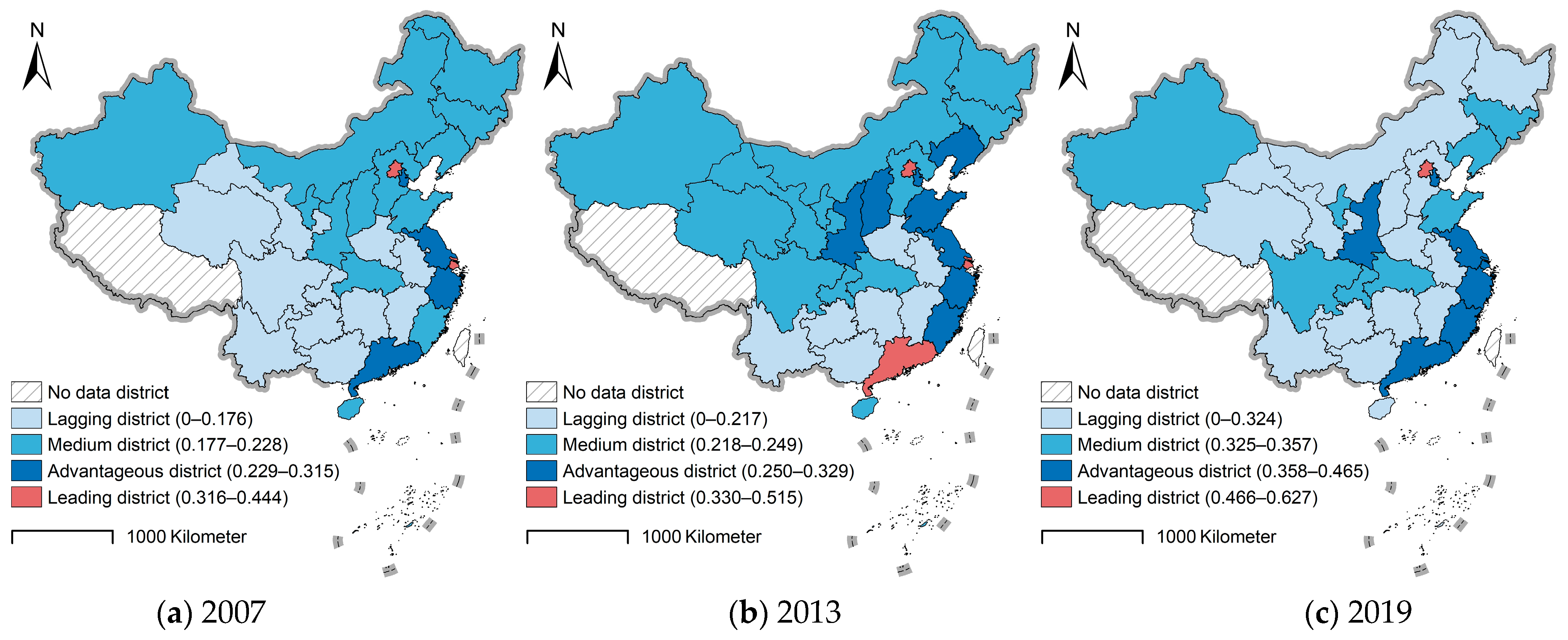
3.2. Spatial Evolution Characteristics

Combining the ArcGIS platform and the natural breaks technique, the HQED level of Chinese provinces was divided into leading, advantageous, medium, and lagging districts, and the spatial visualization results are presented in Figure 2. Considering the regionally uneven impact of the pandemic, the 2020 results do not give a true picture of the recent situation, which requires supplementation with the 2019 results. In general, Chinese HQED has gradually evolved into a development pattern of “only super power and multi-great power” and a spatial pattern of “point, line and plane” from 2007 to 2019, with Beijing as the absolute leader, the southeastern coastal region as the advantageous belt, and the relatively advantageous plane in central and western areas with Shaanxi as the core.

During the period of 2007–2019, HQED evolved from a “dual-core” structure to a “single-core” structure. Beijing and Shanghai have long constituted the principal growth poles of China’s economic development, gathering all kinds of domestic advantageous resources and gaining an absolute advantage in terms of HQED. Particularly, Beijing, as the political, economic, and cultural center of the country, has remained at the national forefront of development, with a primacy that has risen year by year (the primacy ratios, i.e., the ratio between Beijing and the second-ranked province regarding the level of HQED, in 2007, 2013, and 2019 are 1.24, 1.33, and 1.38, respectively). The dual-core structure has gradually been replaced by a single-core structure that manifests spatial characteristics as “points”.

The spatial pattern of a “line” refers to the eastern coastal advantage zone that runs from Guangdong in the southeast, passes through the Yangtze River Delta (YRD), and extends to Bohai Bay in the north. Following the reform and opening-up program, China implemented a strategy of unbalanced regional economic development that prioritizes the eastern part of the country, until the strategies of Western Development (2000), Northeast Revitalization (2003), and Central Rise (2004) were proposed. The accumulation of development advantages over time not only resulted in the eastern region’s advantageous position in the country, but also led to significant inter-regional development gaps. At least at the beginning of the study period (2007), two major economic zones, the Pearl River Delta and the YRD, had been shaped in the eastern region (Figure 2a), which were then connected and extended to the northeast (Figure 2b). However, with the weakening of the policy dividend in the north and the increasing trend of regional synergy and integration in the south, the gap between the northern provinces, such as Shandong and Liaoning, and the southern provinces gradually widened after 2013, and the “line” correspondingly contracted to the southeast coastal advantage belt composed of “multi-great power”, i.e., the five provinces and cities of Jiangsu, Zhejiang, Fujian, Guangdong, and Shanghai (Figure 2c).

Thanks to the advantages of latecomers and the strategy of balanced regional economic development, the central, western, and northeastern regions achieved rapid growth during 2007–2013 (Figure 2a,b), with a trend of catching up with the eastern regions. However, the problem of insufficient core momentums was highlighted as the policy dividend waned, and a district of comparative advantage was developed in central and western China, with Shaanxi as the core, and consisting of Sichuan, Chongqing, Hubei, and Ningxia, as well as the spatial characteristics of a “plane”. In contrast, other extensive lagging “depressions” are characterized by a spatial pattern organized around the central core.

3.3. Spatial Difference Characteristics

DGC, which is represented visually in Figure 3 in figures created using the Origin 2021 platform, was designed to quantify the regional difference in the level of HQED. In general, the national DGC was in the interval of [0.09, 0.16] in 2007–2019, showing a downward trend year by year, with a drop of 42.6%. This reveals that regional disparities and inequalities in HQED are narrowing in China.

Within regions (Figure 3a), the average DGCs of the four major regions from 2007 to 2019 were characterized by a pattern of eastern (0.132) > northeastern (0.049) > western (0.048) > central (0.033). The trend of DGC changes in the eastern, western, and northeastern areas remained in line with the national level, but the western and northeastern regions experienced relatively greater decreases, amounting to 72.71% and 56.05%, respectively. The central region, in contrast, experienced an oscillation after 2014, with a subsequent increase in internal dissimilarity. This could have been associated with the loss of the advantageous position of the resource-based province of Shanxi and its rapid fall into the status of a lagging district.

Inter-regionally (Figure 3b), the HQED level in the eastern part was notably greater than that in other three major regions, leading to a clear regional difference. This is in line with the results of the spatial evolution analysis in the previous section and corroborates Mai et al.’s [8] findings. The DGCs between the eastern–central, eastern–western, and eastern–northeastern regions are in the intervals of [0.12, 0.15], [0.12, 0.23], and [0.13, 0.23], respectively. They all show a decreasing trend, with decreases of 18.88%, 47.05% and 42.03%, respectively. The inter-regional DGCs, except for the eastern region, all fell to within 0.01 in 2019, where an improvement in HQED inequality has been achieved.

Figure 3c further reports the causes of regional differences in the HQED of China. Inter-regional gaps are the primary cause of national DGC inequality, with an average annual contribution of nearly 70% from 2007 to 2019. Intra-regional gaps are the secondary cause, but the contribution rate is trending upward and has recently exceeded 25%, which should be noted by policymakers. However, the contribution of the intensity of trans-variation is on an upward trend, its influence still being relatively limited. This implies a low degree of crossover between different regions for HQED, and indirectly proves the necessity and effectiveness of the balanced regional economic development strategy.

4. Analysis of the Driving Factors of HQED

4.1. Spatial Effects Analysis

The global Moran’s index of HQED levels in Chinese provinces is calculated based on both spatial weight matrices, W_g and W_eg. As shown in

Table 2. Moran’s index of HQED level.

Year	Moran’s Index		Year	Moran’s Index
	Wg	Weg		Wg	Weg
2007	0.314 ***	0.328 ***	2014	0.202 ***	0.281 ***
2008	0.321 ***	0.336 ***	2015	0.191 **	0.274 ***
2009	0.299 ***	0.326 ***	2016	0.140 *	0.239 ***
2010	0.288 ***	0.324 ***	2017	0.160 **	0.241 ***
2011	0.258 ***	0.305 ***	2018	0.136 *	0.228 ***
2012	0.235 ***	0.293 ***	2019	0.099	0.196 ***
2013	0.208 ***	0.275 ***	2020	0.164 **	0.228 ***

Note: ***, **, and * represent significance levels of 1%, 5%, and 10%, respectively.

, Moran’s indices are significantly positive at the 10% level, except for the result of the 2019 W_g matrix. This indicates that the spatial autocorrelation of HQED in China is obvious. Indeed, the high (low) values tend to be clustered, although Moran’s indices are decreasing. Therefore, we can further analyze the driving factors of HQED by employing the spatial econometric model.

4.2. Spatial Effects Analysis

According to the 2007–2020 panel dataset and Stata 17 software, we conducted a likelihood ratio (LR) test, Wald test, Hausman test, and joint test of LR and specific fixed effects using both spatial weight matrices to ensure that the SDM would not degenerate and to determine the particular format of the random or fixed effects. First, the LR test and Wald test rejected the original hypothesis of SDM degradation into spatial lag models and spatial error models with a 1% significance level. Second, the fixed effects model was picked since all of the Hausman test results were positive and significant. Third, the joint test of specific fixed effects and LR further suggests that the use of SDM includes two-way fixed effects of time and region. Overall (

Table 3. Estimation results of SDM at the national level.

Variables	OLS	Wg		Weg
		X	W·X	X	W·X
ρ			−0.236 ***		−0.461 ***
			(−2.58)		(−3.74)
lnPGDP	2.829 ***	2.295 ***	1.682 **	2.275 ***	1.041
	(9.55)	(7.31)	(2.15)	(7.24)	(1.02)
lnURB	0.509 ***	0.443 ***	0.635 ***	0.398 ***	1.233 ***
	(9.42)	(8.18)	(4.40)	(7.17)	(5.96)
lnRES	0.013 **	0.008	−0.020	0.011 **	−0.018
	(2.55)	(1.60)	(−1.56)	(2.32)	(−0.92)
lnGOV	−0.125 ***	−0.136 ***	−0.141 **	−0.146 ***	−0.220 ***
	(−4.92)	(−5.81)	(−2.30)	(−6.42)	(−2.71)
lnINN	0.009	0.015 *	−0.092 ***	0.011	−0.080 ***
	(1.21)	(1.90)	(−5.24)	(1.47)	(−3.21)
lnIND	0.104	0.235	−2.404 ***	0.032	−2.401 **
	(0.45)	(1.08)	(−3.46)	(0.15)	(−2.29)
lnER1	−0.001	0.001	0.008 **	0.001	0.015 **
	(−0.27)	(0.57)	(2.08)	(0.40)	(2.45)
lnER2	−0.008 **	−0.008 ***	0.003	−0.006 *	−0.001
	(−2.37)	(−2.63)	(0.40)	(−1.86)	(−0.01)
R2	0.97	0.93		0.94
LogL	875.91	900.05		903.89
LR-Lag		48.13 ***		55.41 ***
LR-Error		45.77 ***		45.02 ***
Wald-Lag		51.44 ***		60.91 ***
Wald-Error		47.61 ***		47.56 ***
Hausman	75.74 ***	607.19 ***		273.14 ***
LR-FE (Year)		624.59 ***		642.21 ***
LR-FE (Region)		108.29 ***		85.31 ***

Note: ***, **, and * represent significance levels of 1%, 5%, and 10%, respectively. The corresponding statistics are in parentheses.

), the log-likelihoods (LogL) of the SDM estimation based on W_g, W_eg, and the two-way fixed effects were 900.05 and 903.89, respectively, which were greater than those of the non-spatial OLS estimation of 875.91, implying that the SDM estimation is more effective.

As shown in the SDM regression results in Table 3, the coefficient ρ of the spatial lag term of the HQED level is notably negative regardless of the kind of spatial weight matrix, demonstrating that there is an obvious siphon effect of HQED in China. This is contrary to the conclusions of previous studies [47,48], but corroborates the estimation results of Liu and Zhu [49] using spatial Markov chains. On the one hand, for developed regions, the advancement in the HQED level not only implies the expansion of economic scale, but also integrally represents an improvement in residents’ living conditions, the enhancement of social welfare, and the strengthening of the capacity for sustainable growth. The market mechanism will promote the concentration of factors toward advanced productivity, advancing the development of neighboring developed provinces and simultaneously “plundering” the resources and development opportunities of the local provinces. On the other hand, residents, with subjective initiative, will actively move to areas with a higher development level in pursuit of a better quality of life, such as China’s continuous population agglomeration towards the southeastern coastal areas [50]. Losing human capital, notably high-quality human capital, will further aggravate the problems of population aging and insufficient innovation vitality, restraining the HQED of the local provinces. Under the siphon effect, the stronger provinces will become strengthened, and the weaker provinces will weaken, which may eventually evolve into a “core–periphery” structure [51].

4.3. Decomposition of Spatial Effects of SDM Estimation

For further inquiry into both the direct and indirect influences of the studied factors on HQED, and in order to avoid estimation bias due to auto-regression, the partial differentiation method was used to decompose the effects of the explanatory variables, with

Table 4. Decomposition of SDM spatial effects.

Variables	Wg			Weg
	Direct Effects	Indirect Effects	Total Effects	Direct Effects	Indirect Effects	Total Effects
lnPGDP	2.261 ***	1.004	3.265 ***	2.283 ***	0.040	2.323 ***
	(6.62)	(1.55)	(6.43)	(6.50)	(0.05)	(4.00)
lnURB	0.420 ***	0.454 ***	0.874 ***	0.350 ***	0.768 ***	1.118 ***
	(7.40)	(4.06)	(9.15)	(5.90)	(5.06)	(8.69)
lnRES	0.009 **	−0.019 *	−0.009	0.012 ***	−0.016	−0.004
	(2.00)	(−1.78)	(−0.79)	(2.86)	(−1.23)	(−0.27)
lnGOV	−0.132 ***	−0.089 *	−0.220 ***	−0.139 ***	−0.107 *	−0.246 ***
	(−5.64)	(−1.65)	(−4.15)	(−6.10)	(−1.70)	(−4.07)
lnINN	0.018 **	−0.081 ***	−0.063 ***	0.014 **	−0.062 ***	−0.048 ***
	(2.44)	(−5.44)	(−4.59)	(1.97)	(−3.29)	(−2.83)
lnIND	0.338	−2.093 ***	−1.754 ***	0.146	−1.767 **	−1.621 **
	(1.51)	(−3.29)	(−3.08)	(0.66)	(-2.17)	(−2.15)
lnER1	0.001	0.007 **	0.008 **	0.001	0.010 **	0.011 **
	(0.38)	(2.02)	(2.19)	(0.04)	(2.42)	(2.47)
lnER2	−0.008 ***	0.004	−0.004	−0.006 *	0.002	−0.004
	(−2.65)	(0.65)	(−0.70)	(−1.82)	(0.24)	(−0.53)

Note: ***, **, and * represent significance levels of 1%, 5%, and 10%, respectively. The z-statistics are in parentheses.

displaying results.

At the national level, traditional driving factors remain the core factor of China’s HQED during the study period. First, lnPGDP, with regression coefficients greater than 2.2 under both spatial weight matrices, has a significantly direct effect on HQED. This suggests that, despite their obvious differences, economic growth is still the key contributor to HQED, and that for every 1% increase in the former, the latter will increase by more than 2.2%. Secondly, both the direct and indirect influences of lnURB are notably positive, implying that the rise in the level of urbanization in local provinces and neighboring provinces promotes HQED in local provinces. Under the background of upgrading demand structure, rural residents enter the city in pursuit of higher labor-based remuneration and improved living conditions, which directly promotes consumption upgrading and generates spatial spillover effects [52], and further develops benign inter-regional interactions. Thirdly, with technological progress and the extension of industrial chains, the resource advantages of local provinces can be parlayed to some degree into technological and agglomeration advantages. However, the development of neighboring provinces is excessively reliant on resource extraction, triggering serious environmental pollution and inducing negative effects on local provinces, such as air and water pollution with spatial mobility. Therefore, lnRES has a favorable direct effect and a negative indirect effect. Fourth, the expansion of government size causes inefficient investment and corruption problems and leads to lower levels of personal consumption and investment, creating a crowding-out effect, which suppresses residential demand, reduces market dynamics, and increases economic policy uncertainty. This is coupled with the fact that strategic interactions and games between governments may lead to a “race to the bottom”, and thus, both the direct and indirect effects of lnGOV are significantly negative, which further reinforces Chen et al.’s and Ding et al.’s [3] findings.

The contribution of the new momentum to HQED was limited during the study period. On the one hand, although the direct effect of lnINN was notably positive, its contribution to HQED was relatively low compared with that of lnPGDP and lnURB. Due to the inter-regional innovation gap, meanwhile, the indirect effect of lnINN thus showed a siphon effect of neighboring provinces on local provinces. Conversely, the indirect effect of lnIND was notably negative, while the positive direct effect was not significant. This is because industrial structure upgrading breaks the pathway dependence on high-energy-consuming and environmentally damaging sectors, but the transformation and development of local provinces requires a certain economic cycle to generate economic benefits [53]. Under the effects of inter-provincial competition, the modernization of industrial structure in neighboring provinces attracts the resources of local provinces, leading to the loss of resources and inhibiting the HQED of local provinces.

The two types of environmental regulations affect regional HQED to different degrees. The notably positive indirect effect of lnER₁ suggests that command-and-control environmental regulations, for instance, legal and policy constraints, affect HQED primarily in the form of a “pollution halo” effect [54]. Since pollution-intensive enterprises are often resource- and labor-intensive, the mandatory environmental regulation strategy in neighboring provinces forces enterprises to relocate and enter local provinces. In the short term, this leads to more jobs and financial revenue, and fosters economic development. However, the direct effect of lnER₂ is notably negative, which is compatible with the “cost hypothesis”. Cost-based environmental regulation, e.g., emission fees and environmental taxes, directly increases the expenses of innovation and emission control and decreases the market’s and businesses’ profitability and competitiveness, and thus, reduces the productivity of local provinces and hinders HQED. We therefore judged China’s environmental regulations and the level of HQED to have not yet crossed the tipping point of the “environmental Kuznets curve” [55].

4.4. Regional Heterogeneity Analysis

Given the regional inequalities in terms of HQED, it is necessary to conduct a heterogeneity analysis. The optimal model was selected using the spatial weight matrix W_eg, reflecting both geographic and economic distances, as well as the methodology of the previous section. The results of the four regions all suggested the need to employ SDM estimation in a way that includes both temporal and regional two-way fixed effects. Therefore, we further adopted the partial differentiation method to deconstruct the effects, and the outcomes are summarized in

Table 5. Results of SDM estimation and effect decomposition at the regional level.

Variables	Eastern		Central		Western		Northeastern
	Direct Effects	Indirect Effects	Direct Effects	Indirect Effects	Direct Effects	Indirect Effects	Direct Effects	Indirect Effects
ρ		−0.532 ***		−0.542 ***		−0.461***		−0.218
		(−4.11)		(−2.65)		(−2.63)		(−1.42)
lnPGDP	2.607 ***	2.157 **	3.722 ***	−5.380 **	1.593 **	2.771*	9.933 ***	19.442 ***
	(5.33)	(2.01)	(3.73)	(−2.13)	(2.17)	(1.85)	(3.51)	(3.85)
lnURB	−0.027	0.100	−0.406	−2.548 *	0.428 ***	−0.422	3.774 ***	4.843 ***
	(−0.32)	(0.33)	(−0.64)	(−1.65)	(3.48)	(−1.25)	(4.67)	(3.59)
lnRES	0.027 ***	−0.010	0.056 **	−0.103	0.002	0.018	0.116 ***	0.125 ***
	(4.26)	(−0.94)	(1.96)	(−1.49)	(0.29)	(0.98)	(8.54)	(4.23)
lnGOV	−0.042	−0.117	0.048	−0.115	−0.192 ***	−0.080	0.010	0.926 ***
	(−1.12)	(−1.60)	(0.38)	(−0.38)	(−4.10)	(−0.77)	(0.10)	(3.56)
lnINN	0.043 ***	−0.043	0.041 **	0.098 **	0.025 **	0.013	0.286 ***	0.366 ***
	(2.69)	(−1.23)	(2.39)	(2.09)	(2.17)	(0.44)	(4.04)	(3.22)
lnIND	1.767 ***	−2.828 *	−0.111	−5.992 ***	−1.092 ***	−1.194	0.714	−5.588 **
	(4.71)	(−1.81)	(−0.15)	(−3.56)	(−3.00)	(−0.87)	(0.50)	(−2.55)
lnER1	0.008 **	−0.012 **	−0.003	−0.002	0.002	−0.002	0.047 ***	0.049 ***
	(2.33)	(−2.26)	(−0.58)	(−0.18)	(1.01)	(−0.47)	(5.94)	(3.83)
lnER2	0.010 **	0.021 ***	−0.026 ***	−0.006	−0.008*	−0.006	−0.076 ***	−0.081 ***
	(2.47)	(2.59)	(−2.69)	(−0.28)	(−1.65)	(−0.52)	(−5.83)	(−3.90)
R2	0.944		0.911		0.975		0.899
LogL	342.629		206.939		369.771		149.149
LR-Lag	35.76 ***		21.17 ***		25.28 ***		74.34 ***
LR-Error	25.92 ***		18.81 **		31.32 ***		54.98 ***
Wald-Lag	44.21 ***		25.02 ***		27.55 ***		153.52 ***
Wald-Error	29.79 ***		21.13 ***		19.62 **		27.22 ***
Hausman	126.12 ***		95.82 ***		40.60 ***		31.18 ***
LR-FE(Year)	130.31 ***		19.19 **		209.29 ***		19.66 **
LR-FE(Region)	57.05 ***		37.66 ***		53.31 ***		100.23 ***
N	140		84		154		42

Note: ***, **, and * represent significance levels of 1%, 5%, and 10%, respectively. The z-statistics are in parentheses.

.

Corresponding to the characteristics at the national level, the coefficients ρ of the spatial lag term of the HQED level are negative in all four regions (not significant in the northeastern region), suggesting that the core of HQED exerts a siphon effect on neighboring provinces. Although Shanxi and Liaoning had not developed into stable cores and only served as advantageous regions on the national level in 2013 (Figure 2b), their levels of HQED are generally higher than those of other provinces within the regions.

From the perspective of driving factors, the direct effects of lnPGDP, lnRES, and lnINN are all notably positive, proving that economic foundation, natural resources, and innovation capacity are important prerequisites and guarantees for HQED, regardless of region. Meanwhile, there are also significant indirect effects of economic scale in the eastern, western, and northeastern regions, resource endowment in the northeastern region, and green technological innovation in central and northeastern regions.

Furthermore, the urbanization level not only directly promotes HQED in the western and northeastern regions, but also possesses a significant indirect promotion effect in the northeastern region; government size has both a positive direct and a significant indirect effect in the northeastern region, suggesting that HQED in this region may be more dependent on government fiscal expenditure; upgrades to industrial structure breaks path dependence on the existing development patterns in each region, leading to a pain period of adjustment, and the regression coefficient of lnIND is thus negative in most regions. Command-and-control environmental regulation produces a direct compensation mechanism of innovation in the eastern and northeastern regions, which is consistent with Porter’s hypothesis [56]. Conversely, cost-based environmental regulation has a significant direct cost effect and an indirect “pollution haven” effect [54] in regions other than the east.

5. Conclusions and Policy Implications

5.1. Conclusions

Combining the indicator system developed via the assessment of ERG needs and various weighting strategies, this paper evaluates the level of HQED at the provincial level in China from 2007 to 2020, reveals the characteristics of spatial–temporal evolution, and analyzes the driving mechanism. The primary conclusions are as follows.

First, from 2007 to 2019, the aggregate HQED level of Chinese provinces increased from 0.211 to 0.348 with an average yearly growth rate of 4.18%, indicating a consistent increasing trend, with the exception of the shock caused by COVID-19 in 2020. In this process, the development pattern of “only super power and multi-great power” and the spatial characteristics of “point, line, and plane” gradually developed, with Beijing as the absolute leader, the southeastern coastal region as the advantageous belt, and the relatively advantageous plane in central and western areas with Shaanxi as the core. The spatial–temporal evolutionary features of HQED corroborate the existing results [26], and the case study of Li et al. [25] provides additional mesolevel evidence for these findings.

Second, DGC lay in the interval of [0.09, 0.16] and decreased with time, demonstrating that the spatial differences in HQED in China gradually narrowed, while regional coordination increased. The within-region differences in the four regions were organized in order of eastern > northeastern > western > central. Although the central, western, and northeastern regions achieved swift development during the study period, they still significantly differed from the eastern region. Consistent with the findings of Mai et al. [8], these gaps were the dominant contributors to the headline DGC.

Third, at the national level, the Chinese provincial level of HQED displayed significant spatial autocorrelation. This was revealed to be a siphon effect using the SDM estimator. Moreover, economic scale, urbanization level, and resource endowment, as important prerequisites and guarantees, exerted significant direct promotion effects on HQED, but only the indirect impact of urbanization level was notably positive. The advancement effect of green technology innovation on local provinces’ HQED began to appear, but the indirect effect, like that of upgrading industrial structure, today remains significantly negative. Local regions were unaffected by command-and-control environmental regulation, but the impact of increased regulatory intensity in neighboring regions on local regions was consistent with the “pollution halo” hypothesis. Meanwhile, cost-based environmental regulation suppressed HQED in local provinces under the cost effect. The expansion of government size significantly inhibited local provinces’ HQED, both directly and indirectly, due to excessive intervention in the economy, which inhibited market dynamics and residential needs. The findings of the OLS estimator confirmed the above conclusions [26], and we further revealed more details about the spatial impact of the variables.

Fourth, the regional heterogeneity analysis based on the SDM estimator revealed that spatial factors significantly affected HQED in four primary regions. The coefficients of the spatial lag terms of HQED levels in four major regions were all negative, but only not significant in the northeastern region. This suggests that provinces with higher HQED levels may exert a siphon effect on neighboring provinces with lower levels, which is similar to the results of the national-level estimation. Each region sees economic scale, resource endowment, and green technology innovation drive HQED, while the indirect effects are regionally heterogeneous. The level of urbanization not only contributes directly to HQED in the western and northeastern regions, but also significantly contributes indirectly to the northeastern region; government size has both direct and indirect benefits only in the northeastern region, which may be associated with the region’s dependence on government fiscal expenditure. Additionally, although not fully significant, industrial structure upgrading, command-and-control, and cost-based environmental regulations have essentially negative direct and indirect effects outside the eastern region. This suggests that, for less developed regions with predominantly resource- and pollution-intensive industries, the disruption of smooth growth paths and cost upgrading acts as a constraint on HQED, at least in the short term.

5.2. Policy Implications

Based on the above findings, we make the following policy recommendations.

First, it is necessary to adhere to the people’s well-being in the orientation of development, while also working to stabilize the speed and increase the quality of economic growth. The HQED level of Chinese provinces, with a peak value of 0.627 and an average value of 0.348 in 2019, still has extensive potential for improvement. This will require society to address its principal contradictions by improving the income distribution mechanism, raising the real income level of residents, committing to overcoming the problem of relative poverty on the basis of eliminating absolute poverty, upgrading the level of public services to meet the diversified needs of residents, and setting up a supporting performance appraisal system.

Second, the authorities should coordinate regional coordinated development and reduce regional development inequality. On the one hand, this must entail increasing the policy inclination to lagging regions, reversing the siphon effect of HQED into a spatial spillover effect, and giving play to the radiation effect of developed regions on lagging ones. On the other hand, local governments must strengthen inter-regional exchanges and cooperation, weaken local protection and trade barriers, accelerate the inter-regional flow of production factors (such as capital and technological advantages in the eastern region, and labor and resource advantages in the central, western, and northeastern regions), give full play to the advantages of regional characteristics and comparative advantages according to local conditions, and promote the regional division of labor and upstream and downstream industrial cooperation.

Third and finally, it is necessary to accelerate the transformation of development momentums and strengthen ecological and environmental constraints. In the new era of development, it is necessary to improve the socialist market economic system, strengthen the protection of intellectual property rights and patents, improve market vitality and operational efficiency, drive the overall upgrading of the industrial structure with technological innovation, and promote the succession and conversion of old and new momentums. Meanwhile, authorities should adhere to the concept of green development, improve ecological compensation and incentive mechanisms to reduce consumption, prevent the “race to the bottom” and “shadow economy”, and accelerate the crossing of the “environmental Kuznets curve” inflection point.

References

1. Wang, D.Q.; Xue, S.C.; Lu, Z.H.; Zhou, Y.H.; Hou, Y.W.; Guo, M.X. Dynamic evolution and spatial-temporal disparities decomposition of high-quality economic development in China. Environ. Dev. Sustain. 2023, 1–29. [Google Scholar] [CrossRef]
2. Guo, B.N.; Wang, Y.; Zhang, H.; Liang, C.Y.; Feng, Y.; Hu, F. Impact of the digital economy on high-quality urban economic development: Evidence from Chinese cities. Econ. Model. 2023, 120, 106194. [Google Scholar] [CrossRef]
3. Ding, C.H.; Liu, C.; Zheng, C.Y.; Li, F. Digital economy, technological innovation and high-quality economic development: Based on spatial effect and mediation effect. Sustainability 2022, 14, 216. [Google Scholar] [CrossRef]
4. Mishan, B. The Costs of Economic Growth, 2nd ed.; F. A. Praeger: Westport, CT, USA, 1993. [Google Scholar]
5. Kamaev, B.D. Speed and Quality of Economic Growth; Hubei People’s Publishing House: Wuhan, China, 1983. [Google Scholar]
6. Pang, J.N.; Jiao, F.Y.; Zhang, Y.M. An analysis of the impact of the digital economy on high-quality economic development in china-a study based on the effects of supply and demand. Sustainability 2022, 14, 16991. [Google Scholar] [CrossRef]
7. Yang, Y.W.; Zhang, P. Logic, measurement and governance in China’s high-quality economic development. Econ. Res. J. 2021, 56, 26–42. [Google Scholar]
8. Mai, Q.; Bai, M.; Li, L. Study on the dynamic evolution and regional differences of the level of high-quality economic and social development in China. Sustainability 2023, 15, 382. [Google Scholar] [CrossRef]
9. Barro, R.J. Quantity and quality of economic growth; Banco Central de Chile: Santiago, Chile, 2002. [Google Scholar]
10. Thomas, V.; Dailami, M.; Dhareshwar, A.; López, R.; Kaufmann, D.; Kishor, N.; Wang, Y. The Quality of Growth; Oxford University Press: New York, NY, USA, 2000. [Google Scholar]
11. Wei, M.; Li, S. Research on the measurement of the high quality development level of China’s economy in the new era. J. Quant. Tech. Econ. 2018, 35, 3–20. [Google Scholar]
12. Wang, J.W.; Gao, X.X.; Jia, R.H.; Zhao, L.S. Evaluation index system construction of high-quality development of Chinese real enterprises based on Factor Analysis and AHP. Discret. Dyn. Nat. Soc. 2022, 2022, 8733002. [Google Scholar] [CrossRef]
13. He, H.; Tuo, S.H.; Lei, K.W.; Gao, A.X. Assessing quality tourism development in China: An analysis based on the degree of mismatch and its influencing factors. Environ. Dev. Sustain. 2023, 1–28. [Google Scholar] [CrossRef]
14. Han, J.; Zheng, Q.; Xie, D.; Muhammad, A.; Isik, C. The construction of green finance and high-quality economic development under China’s SDGs target. Environ. Sci. Pollut. Res. 2023, 30, 111891–111902. [Google Scholar] [CrossRef]
15. Chen, T.Y.; Zhou, Y.K.; Zou, D.; Wu, J.T.; Chen, Y.; Wu, J.P.; Wang, J. Deciphering china’s socio-economic disparities: A comprehensive study using nighttime light data. Remote Sens. 2023, 15, 4581. [Google Scholar] [CrossRef]
16. Chisadza, C.; Bittencourt, M. Economic development and democracy: The modernization hypothesis in sub-Saharan Africa. Soc. Sci. J. 2019, 56, 243–254. [Google Scholar] [CrossRef]
17. Ma, T.; Cao, X.X.; Zhao, H. Development zone policy and high-quality economic growth: Quasi-natural experimental evidence from China. Reg. Stud. 2023, 57, 590–605. [Google Scholar] [CrossRef]
18. Zhu, Y.; Bashir, S.; Marie, M. Assessing the relationship between poverty and economic growth: Does sustainable development goal can be achieved? Environ. Sci. Pollut. Res. 2022, 29, 27613–27623. [Google Scholar] [CrossRef]
19. Liu, Y.; Liu, M.; Wang, G.G.; Zhao, L.L.; An, P. Effect of environmental regulation on high-quality economic development in China: An empirical analysis based on dynamic spatial Durbin model. Environ. Sci. Pollut. Res. 2021, 28, 54661–54678. [Google Scholar] [CrossRef]
20. Ghatak, M. Measures of Development—Concepts, Causality, and Context. In Economics, Management and Sustainability: Essays in Honour of Anup Sinha; Springer: Singapore, 2018. [Google Scholar]
21. Human Development Report. Available online: https://www.undp.org/somalia/publications/human-development-report-2022 (accessed on 19 September 2023).
22. Szopik-Depczynska, K.; Cheba, K.; Bak, I.; Stajniak, M.; Simboli, A.; Ioppolo, G. The study of relationship in a hierarchical structure of EU sustainable development indicators. Ecol. Indic. 2018, 90, 120–131. [Google Scholar] [CrossRef]
23. Bates, W. Gross national happiness. Asian-Pac. Econ. Lit. 2009, 23, 1–16. [Google Scholar] [CrossRef]
24. Li, X.S.; Lu, Y.L.; Huang, R.T. Whether foreign direct investment can promote high-quality economic development under environmental regulation: Evidence from the Yangtze River Economic Belt, China. Environ. Sci. Pollut. Res. 2021, 28, 21674–21683. [Google Scholar] [CrossRef]
25. Li, C.; Peng, W.; Shen, X.; Gu, J.; Zhang, Y.; Li, M. Comprehensive evaluation of the high-quality development of the ecological and economic belt along the Yellow River in Ningxia. Sustainability 2023, 15, 11486. [Google Scholar] [CrossRef]
26. Chen, L.; Huo, C. The measurement and influencing factors of high-quality economic development in China. Sustainability 2022, 14, 9293. [Google Scholar] [CrossRef]
27. Tanaka, K.; Managi, S. Industrial agglomeration effect for energy efficiency in Japanese production plants. Energy Policy 2021, 156, 112442. [Google Scholar] [CrossRef]
28. Bloom, D.E.; Chatterji, S.; Kowal, P.; Lloyd-Sherlock, P.; McKee, M.; Rechel, B.; Rosenberg, L.; Smith, J.P. Macroeconomic implications of population ageing and selected policy responses. Lancet 2015, 385, 649–657. [Google Scholar] [CrossRef]
29. Chen, B.K.; Lin, J.Y. Development strategy, resource misallocation and economic performance. Struct. Chang. Econ. Dyn. 2021, 59, 612–634. [Google Scholar] [CrossRef]
30. Khan, M. CO2 emissions and sustainable economic development: New evidence on the role of human capital. Sustain. Dev. 2020, 28, 1279–1288. [Google Scholar] [CrossRef]
31. Fu, Y.; Zhuang, H.T.; Zhang, X.F. Do environmental target constraints of local government affect high-quality economic development? Evidence from China. Environ. Sci. Pollut. Res. 2023, 30, 56620–56640. [Google Scholar] [CrossRef] [PubMed]
32. Kubiszewski, I.; Costanza, R.; Franco, C.; Lawn, P.; Talberth, J.; Jackson, T.; Aylmer, C. Beyond GDP: Measuring and achieving global genuine progress. Ecol. Econ. 2013, 93, 57–68. [Google Scholar] [CrossRef]
33. Alderfer, C.P. An empirical test of a new theory of human needs. Organ. Behav. Hum. Perform. 1969, 4, 142–175. [Google Scholar] [CrossRef]
34. Schneider, B.; Alderfer, C.P. Three Studies of Measures of Need Satisfaction in Organizations. Adm. Sci. Q. 1973, 18, 489–505. [Google Scholar] [CrossRef]
35. Yang, C.-L.; Hwang, M.; Chen, Y.-C. An empirical study of the existence, relatedness, and growth (ERG) theory in consumer’s selection of mobile value-added services. Afr. J. Bus. Manag. 2011, 5, 7885–7898. [Google Scholar]
36. Bain, P.G.; Bongiorno, R. Evidence from 33 countries challenges the assumption of unlimited wants. Nat. Sustain. 2022, 5, 669–673. [Google Scholar] [CrossRef]
37. Diakoulaki, D.; Mavrotas, G.; Papayannakis, L. Determining objective weights in multiple criteria problems: The CRITIC method. Comput. Oper. Res. 1995, 22, 763–770. [Google Scholar] [CrossRef]
38. Krishnan, A.R.; Kasim, M.M.; Hamid, R.; Ghazali, M.F. A modified CRITIC method to estimate the objective weights of decision criteria. Symmetry 2021, 13, 973. [Google Scholar] [CrossRef]
39. Dagum, C. A new approach to the decomposition of the Gini income inequality ratio. Empir. Econ. 1997, 22, 515–531. [Google Scholar] [CrossRef]
40. Nembua, C.C. The multi-decomposition of the Hirschman-Herfindahl index: Measuring household inequality in Cameroon, 1996–2001. Appl. Econ. Lett. 2007, 14, 27–34. [Google Scholar] [CrossRef]
41. LeSage, J.P.; Pace, R.K. Introduction to Spatial Econometrics; CRC Press: Boca Raton, FL, USA, 2009. [Google Scholar]
42. Zhang, Z.; Wei, X. Spatial spillover effects of national-level eco-industrial park establishment on regional ecological efficiency: Evidence from 271 cities in China. Environ. Sci. Pollut. Res. 2023, 30, 62440–62460. [Google Scholar] [CrossRef]
43. Lin, B.Q.; Ma, R.Y. Green technology technology innovations, urban innovation environment and CO2 emission reduction in China: Fresh evidence from a partially linear functional-coefficient panel model. Technol. Forecast. Soc. Chang. 2022, 176, 121434. [Google Scholar] [CrossRef]
44. Anselin, L. Spatial Econometrics: Methods and Models; Kluwer Academic Publishers: New York, NY, USA, 1988. [Google Scholar]
45. Guo, J.; Sun, Z. How does manufacturing agglomeration affect high-quality economic development in China? Econ. Anal. Policy 2023, 78, 673–691. [Google Scholar] [CrossRef]
46. Liu, S. The impact of COVID-19 on China’s regional economy. Geogr. Res. 2021, 40, 310–325. [Google Scholar]
47. Gao, J.; Wu, D.L.; Xiao, Q.; Randhawa, A.; Liu, Q.; Zhang, T. Green finance, environmental pollution and high-quality economic development-a study based on China’s provincial panel data. Environ. Sci. Pollut. Res. 2023, 30, 31917–31939. [Google Scholar] [CrossRef]
48. Zhang, J.; Yuan, J.D.; Wang, Y.C. Spatio-temporal evolution and influencing factors of coupling coordination between urban resilience and high-quality development in Yangtze River Delta Area, China. Front. Environ. Sci. 2023, 11, 1174875. [Google Scholar] [CrossRef]
49. Liu, P.D.; Zhu, B.Y. Temporal-spatial evolution of green total factor productivity in China’s coastal cities under carbon emission constraints. Sust. Cities Soc. 2022, 87, 104231. [Google Scholar] [CrossRef]
50. Teng, F.; Wang, Y.J.; Wang, M.J.; Wang, L.Q. Monitoring and analysis of population distribution in China from 2000 to 2020 based on remote sensing data. Remote Sens. 2022, 14, 6019. [Google Scholar] [CrossRef]
51. Krugman, P. Increasing returns and economic geography. J. Polity Econ. 1991, 99, 483–499. [Google Scholar] [CrossRef]
52. Cheng, K.M.; Liu, S.C. Does urbanization promote the urban-rural equalization of basic public services? Evidence from prefectural cities in China. Appl. Econ. 2023, 1–15. [Google Scholar] [CrossRef]
53. Yang, Z. The impact of green finance on high-quality economic development in China: Vertical fiscal imbalance as the moderating effect. Sustainability 2023, 15, 9350. [Google Scholar] [CrossRef]
54. Zheng, H.; Zhang, L.; Song, W.L.; Mu, H.R. Pollution heaven or pollution halo? Assessing the role of heterogeneous environmental regulation in the impact of foreign direct investment on green economic efficiency. Environ. Sci. Pollut. Res. 2023, 30, 21619–21637. [Google Scholar] [CrossRef]
55. Ahmad, M.; Jabeen, G.; Wu, Y.Y. Heterogeneity of pollution haven/halo hypothesis and Environmental Kuznets Curve hypothesis across development levels of Chinese provinces. J. Clean. Prod. 2021, 285, 124898. [Google Scholar] [CrossRef]
56. Porter, M.E.; Linde, C.V.D. Toward a new conception of the environment competitiveness relationship. J. Econ. Perspect. 1995, 9, 97–118. [Google Scholar] [CrossRef]
Figure 1. Time-series evolution of HQED levels at different spatial scales in China, 2007–2020.
Sustainability 15 16308 g001
Figure 2. Spatial pattern of the HQED level in Chinese provinces in 2007, 2013, and 2019.
Sustainability 15 16308 g002
Figure 3. Regional differences and drivers of HQED in China. Note: eastern, central, western, and northeastern regions are symbolized by the letters E, C, W, and N, respectively.
Sustainability 15 16308 g003