
Confidence in Greenhouse Gas Emission Estimation: A Case Study of Formaldehyde Manufacturing

 , , and
Abstract
:1. Introduction
2. Materials and Methods
2.1. Scope of Analysis
2.2. The Formaldehyde Production Process through the “Oxide Route”
2.3. The Method to Estimate Direct Emissions in Formaldehyde Production
- M = mass of CO2 emitted during the period (in t).
- Qmean = average hourly flow rate during the period (in N m3/h).
- V = CO2 concentration in exhaust gases (in N m3/N m3).
- h = number of production hours during the period (in hours).
- r = conversion factor from Nm3 of CO2 to tons of CO2 (in t/N m3).
- k = adjustment factor for the Clapeyron formula (in K/K).
- P = average daily production of formaldehyde during the period (t/day).
2.4. Statistical Model
2.4.1. The Expected Value of M
- The mean and standard deviation of P, V, h, and 1/T.
- The covariances among these variables.
2.4.2. The Variance of M
2.4.3. Data Gathering
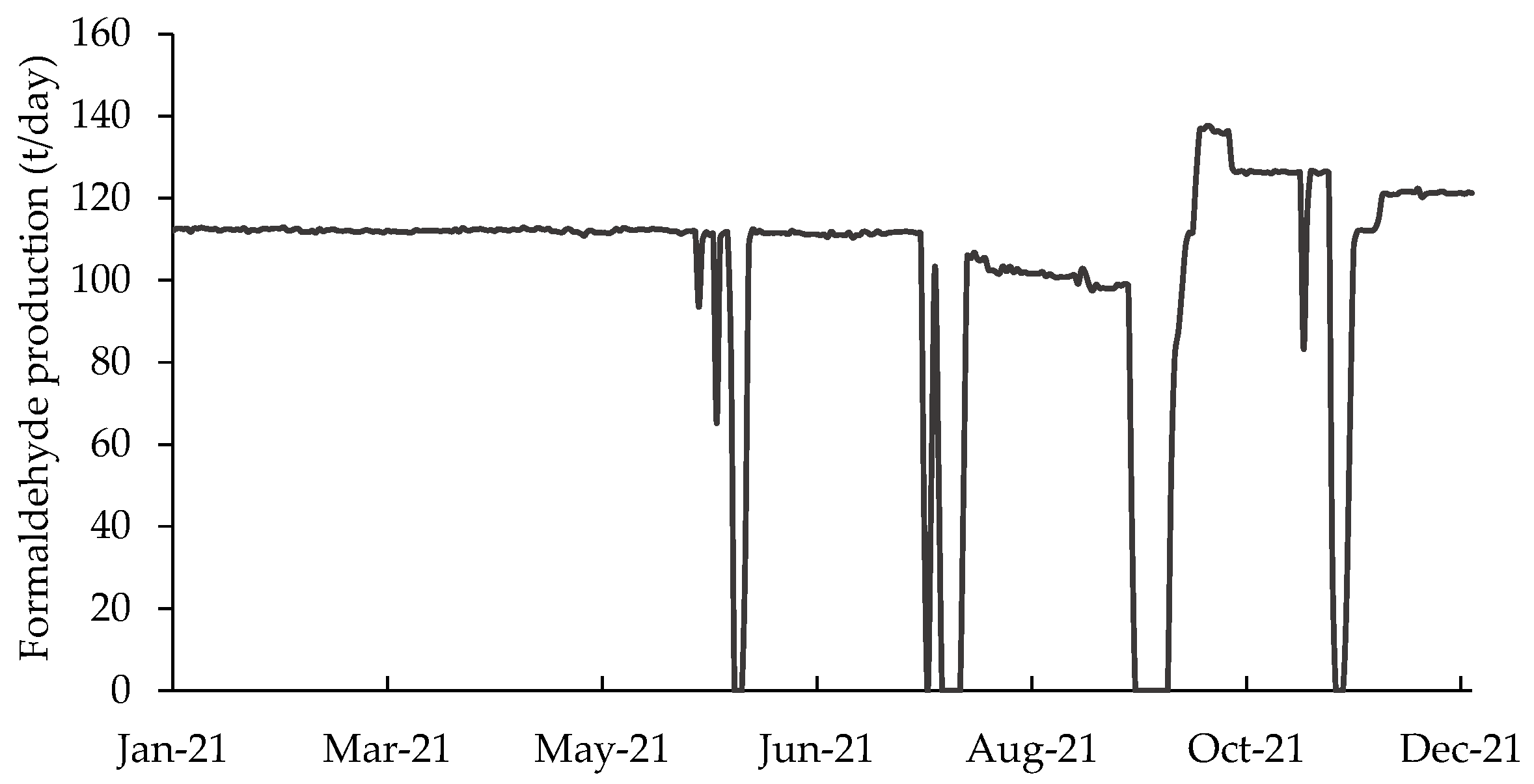
- P—The daily production was directly measured according to the company’s management system records from 1 January to 31 December 2021. The value of the formaldehyde production in tons is considered quite accurate for long periods. For short periods (such as a day), there may be distortions between actual and recorded values. These variations cancel out the accumulated values produced over long periods. P was considered a normal random variable whose mean and standard deviation remained constant throughout the year. The average hourly flow rate during production periods was estimated without considering the variation of P caused by interruptions and resumptions of activity. Variations in production due to interruptions and resumptions were captured in the computation of the number of h. The value of P was used to calculate the Qmean during a day, and h was used to estimate the time in which this flow was practiced during the day. Thus, the uncertainty about the value of P affected the uncertainty about the value of the hourly flow, which was controlled to correspond to approximately 90% of the maximum design flow.
- V—Volumetric concentration measurements were made by laboratory analysis using gas chromatography, which exhibits a high degree of precision. The volumetric concentration of CO2 corresponds to the average value of the readings during operations throughout the year. Therefore, V was considered a normal variable with a constant mean and standard deviation throughout the year.
- h—The number of hours worked per day was a variable recorded by the company’s management and is subject to imprecision due to approximations and measurement errors. For example, some hours worked in a given month could be recorded in the subsequent month, or vice versa. Deviation in the recording of production hours was possible when there were interruptions in production, and it was difficult to determine when the counting of production time should begin as the process required a certain interval of time to stabilize.
- 1/T—The temperature measurement of exhaust gases should remain controlled at 120 °C (393.15 K). However, variations in the process, load, flow, or even external temperature can affect this temperature. We consider that 1/T is a normal variable and that its mean and standard deviation remain constant throughout the year.
2.4.4. Correlations between the Variables
3. Results
3.1. Means and Uncertainties in the Measurements
3.1.1. Measurements of P
3.1.2. Measurements of V
3.1.3. Measurements of h
3.1.4. Measurements of 1/T
3.2. Correlations between the Variables
- One possibility of correlation is that the measurements for determining the variables P, V, h, and 1/T use instruments subject to systematic errors. We found no indication of the occurrence of such a possibility, and, thus, such a reason for correlations was discarded.
- The correlation between the values of h and the other variables should be disregarded. Thus, we will consider h as independent from the others.
- The correlations between P and the variables T and V were also disregarded because of the following argument: Indeed, the temperature T and the concentration V depend on the production level P. However, in practice, once it is identified that the production level changes, process management commands adjustments to control the process, and, therefore, T and V are controlled. Thus, we will consider that P is independent of the other variables.
- Between T and V, it was considered that there is an important correlation since the temperature increases when the level of residual gases increases. Therefore, conservatively, we assume that the correlation between 1/T and V is equal to −1.
3.3. Estimation of Mean and Variance of the Emission
4. Discussion
4.1. Known and Unknown Uncertainties
4.2. The Effect of Correlations
4.3. Length of the Period of Analysis
4.4. Control of the Process and Precision
4.5. Comparison with Other Emission Estimates
5. Conclusions
Supplementary Materials
Author Contributions
Funding
Institutional Review Board Statement
Informed Consent Statement
Data Availability Statement
Acknowledgments
Conflicts of Interest
References
- Kauffmann, C.; Less, C.T.; Teichmann, D. Corporate Greenhouse Gas Emission Reporting: A Stocktaking of Government Schemes; OECD Working Papers on International Investment No. 2012/01; OECD Publishing: Paris, France, 2012; 74p. [Google Scholar]
- Inakollu, S.; Morin, R.; Keefe, R. Carbon Footprint Estimation in Fiber Optics Industry: A Case Study of OFS Fitel, LLC. Sustainability 2017, 9, 865. [Google Scholar] [CrossRef]
- Carbon Disclosure Project (CDP). Global 500 Report; CDP: London, UK, 2009; 49p. [Google Scholar]
- Fonseca, R.C.; Indicadores de Sustentabilidade Empresarial de Boas Práticas para Micro e Pequenas Empresas: Análise Crítica e Framework Conceitual. Universidade Tecnológica Federal do Paraná, [S. L.]. 2020. Available online: https://utfws.utfpr.edu.br/acad01/sistema/mpCadDefQualPg.pcTelaAss (accessed on 20 February 2023).
- Yona, L.; Cashore, B.; Jackson, R.B.; Ometto, J.; Bradford, M.A. Refining national greenhouse gas inventories. Ambio 2020, 49, 1581–1586. [Google Scholar] [CrossRef] [PubMed]
- Tonin, S.; La Notte, A.; Nocera, S. A use-chain model to deal with uncertainties. A focus on GHG emission inventories. Carbon Manag. 2016, 7, 347–359. [Google Scholar] [CrossRef]
- Intergovernmental Panel on Climate Change (IPCC). IPCC Guidelines for National Greenhouse Gas Inventories. Volume 1: General Guidance and Reporting. Kanagawa: IPCC Guidelines for National Greenhouse Gas Inventories, National Greenhouse Gas Inventories Programme. 2006. Available online: https://www.ipcc-nggip.iges.or.jp/public/2006gl/vol1.html (accessed on 6 April 2023).
- Brandon, R.G.; Krueger, P.; Schmidt, P.S. ESG Rating Disagreement and Stock Returns; Finance Working Paper No. 651/2020; European Corporate Governance Institute: Brussels, Belgium, 2021; 57p. [Google Scholar] [CrossRef]
- Carotenuto, F.; Gualtieri, G.; Miglietta, F.; Riccio, A.; Toscano, P.; Wohlfahrt, G.; Gioli, B. Industrial point source CO2 emission strength estimation with aircraft measurements and dispersion modelling. Environ. Monit. Assess. 2018, 190, 165. [Google Scholar] [CrossRef] [PubMed]
- Jonas, M.; Marland, G.; Krey, V.; Wagner, F.; Nahorski, Z. Uncertainty in an emissions-constrained world. Clim. Chang. 2014, 124, 459–476. [Google Scholar] [CrossRef]
- Lesiv, M.; Bun, A.; Jonas, M. Analysis of change in relative uncertainty in GHG emissions from stationary sources for the EU 15. Clim. Chang. 2014, 124, 505–518. [Google Scholar] [CrossRef]
- Keoleian, G.A.; Spitzley, D.V. Chapter 7 Life cycle-based sustainability metrics. Sustain. Sci. Eng. 2006, 1, 127–159. [Google Scholar] [CrossRef]
- Lima, R.S.; Caldeira-Pires, A.A.; Cardoso, A.N. Uncertainty analysis in Life Cycle Assessment applied to biorefineries systems: A critical review of the literature. Process Integr. Optim. Sustain. 2020, 4, 1–13. [Google Scholar] [CrossRef]
- Park, Y.S.; Yeon, S.M.; Lee, G.Y.; Park, K.H. Proposed Consecutive Uncertainty Analysis Procedure of the Greenhouse Gas Emission Model Output for Products. Sustainability 2019, 11, 2712. [Google Scholar] [CrossRef]
- Igos, E.; Benetto, E.; Meyer, R.; Baustert, P.; Othoniel, B. How to treat uncertainties in Life Cycle Assessment studies. Int. J. Life Cycle Assess. 2019, 24, 794–807. [Google Scholar] [CrossRef]
- Marujo, E.C.; Rodrigues, G.G.; Amaral, W.A.N.; Leonardis, F.; Covatti, A. A procedure to estimate variances and covariances on GHG emissions and inventories. Carbon Manag. 2022, 13, 310–320. [Google Scholar] [CrossRef]
- Tang, X.; Bai, Y.; Duong, A.; Smith, M.T.; Li, L.; Zhang, L. Formaldehyde in China: Production, consumption, exposure levels, and health effects. Environ. Int. 2009, 3, 1210–1224. [Google Scholar] [CrossRef] [PubMed]
- Bahmanpour, A.M.; Hoadley, A.; Tanksale, A. Critical review and exergy analysis of formaldehyde production processes. Rev. Chem. Eng. 2014, 30, 583–604. [Google Scholar] [CrossRef]
- Greenhouse Gas Protocol Initiative (GHG). A Corporate Accounting and Reporting Standard; World Resources Institute and World Business Council for Sustainable Development: Geneva, Switzerland, 2004. [Google Scholar]
- Style, R.W.; Gerber, D.; Rempel, A.W.; Dufresne, E.R. The generalized Clapeyron equation and its application to confined ice growth. arXiv 2023, arXiv:2301.03895. [Google Scholar] [CrossRef]
- Bohrnstedt, G.W.; Goldberger, A.S. On the Exact Covariance of Products of Random Variables. J. Am. Stat. Assoc. 1969, 64, 1439–1442. [Google Scholar] [CrossRef]
- Intergovernmental Panel on Climate Change (IPCC). Good Practice Guidance and Uncertainty Management in National Greenhouse Gas Inventorie; Penman, J., Kruger, D., Galbally, I., Hiraishi, R., BYenzi, B., Emmanul, S., Buendia, L., Hoppaus, R., Martinsen, T., Meijer, J., et al., Eds.; Institute for Global Environmental Strategies: Hayama, Japan, 2000. [Google Scholar]
- Giordano, M. Uncertainty propagation with functionally correlated quantities. arXiv 2016, arXiv:1610.08716. [Google Scholar]
- Molina-Castro, G. A Monte Carlo Method for Quantifying Uncertainties in The Official Greenhouse Gas Emission Factors Database of Costa Rica. Front. Environ. Sci. 2022, 10, 896256. [Google Scholar] [CrossRef]
- Groen, E.A.; Heijungs, R. Ignoring correlation in uncertainty and sensitivity analysis in life cycle assessment: What is the risk? Environ. Impact Assess. Rev. 2017, 62, 98–109. [Google Scholar] [CrossRef]
- Barahmand, Z.; Eikeland, M.S. Life Cycle Assessment under Uncertainty: A Scoping Review. World 2022, 3, 39. [Google Scholar] [CrossRef]
- Devore, J.L. Probability and Statistics for Engineering and the Sciences, 8th ed.; Cengage Learning: Belmont, CA, USA, 2012. [Google Scholar]
- Wiki R Contributors. Teste Shapiro-Wilk (Ryan-Joiner). 2021. Available online: https://www.ufrgs.br/wiki-r/index.php?title=Teste_Shapiro-Wilk_(Ryan-Joiner)&oldid=3247 (accessed on 20 February 2023).


| Variable | Mean | Unit of Measurement | Standard Deviation | Standard Deviation/Mean % |
|---|---|---|---|---|
| P | 111.97 | t/day | 1.57 | 1.4% |
| 1/T | 0.00254 | 1/K | 0.00006 | 2.5% |
| H | 8.278 | hour/year | 83 | 1.0% |
| V | 0.01444 | m3/m3 | 0.29 | 20% |
| P | 1/T | H | V | |
|---|---|---|---|---|
| P | 1 | 0 | 0 | 0 |
| 1/T | 0 | 1 | 0 | −1 |
| H | 0 | 0 | 1 | 0 |
| V | 0 | −1 | 0 | 1 |
| This Report (A) | Own Company (B) | Third-Party (C) |
|---|---|---|
| 970 | 938 | 1434 |
Disclaimer/Publisher’s Note: The statements, opinions and data contained in all publications are solely those of the individual author(s) and contributor(s) and not of MDPI and/or the editor(s). MDPI and/or the editor(s) disclaim responsibility for any injury to people or property resulting from any ideas, methods, instructions or products referred to in the content. |
© 2023 by the authors. Licensee MDPI, Basel, Switzerland. This article is an open access article distributed under the terms and conditions of the Creative Commons Attribution (CC BY) license (https://creativecommons.org/licenses/by/4.0/).
Share and Cite
Marujo, E.C.; Almeida, J.R.U.C.; Souza, L.F.L.; Costa, A.R.S.P.; Miranda, P.C.G.; Covatti, A.A.; Holschuch, S.G.; Melo, P.M.S. Confidence in Greenhouse Gas Emission Estimation: A Case Study of Formaldehyde Manufacturing. Sustainability 2023, 15, 16578. https://doi.org/10.3390/su152416578
Marujo EC, Almeida JRUC, Souza LFL, Costa ARSP, Miranda PCG, Covatti AA, Holschuch SG, Melo PMS. Confidence in Greenhouse Gas Emission Estimation: A Case Study of Formaldehyde Manufacturing. Sustainability. 2023; 15(24):16578. https://doi.org/10.3390/su152416578
Chicago/Turabian StyleMarujo, Ernesto C., José R. U. C. Almeida, Luiz F. L. Souza, Alan R. S. P. Costa, Paulo C. G. Miranda, Arthur A. Covatti, Solange G. Holschuch, and Potira M. S. Melo. 2023. "Confidence in Greenhouse Gas Emission Estimation: A Case Study of Formaldehyde Manufacturing" Sustainability 15, no. 24: 16578. https://doi.org/10.3390/su152416578
APA StyleMarujo, E. C., Almeida, J. R. U. C., Souza, L. F. L., Costa, A. R. S. P., Miranda, P. C. G., Covatti, A. A., Holschuch, S. G., & Melo, P. M. S. (2023). Confidence in Greenhouse Gas Emission Estimation: A Case Study of Formaldehyde Manufacturing. Sustainability, 15(24), 16578. https://doi.org/10.3390/su152416578