Methane Exchange Flux Monitoring between Potential Source Sewage Inspection Wells and the Atmosphere Based on Laser Spectroscopy Method

Abstract

Greenhouse gas emissions are changing the climate and affecting human activities. In cities, the anaerobic environment in sewage inspection wells produces CH₄, which is exchanged with the atmosphere and causes pollution. Moreover, although the number of inspection wells has increased with the development of cities, people have not paid enough attention to this potential source of CH₄ and ignored it in the statistics of greenhouse gas inventories. Conventional gas monitoring methods like gas chromatography are complex and expensive. Based on the portable TDLAS CH₄ sensor developed by our team, combined with a gas velocity analyser, we realised in situ continuous flux monitoring. We corrected the effect of temperature on the results according to the theory of infrared thermometry. We showed that the measurement results of the sensor fluctuate within the range of ±0.1 ppm of the measured standard gas concentration. We also verified its repeatability and ensured its reliability in field applications by comparing its results with the results of gas chromatography analysis. In addition to flux monitoring, based on the monitoring data of 56 inspection wells in the study area, the average concentration was estimated using the Bootstrap method, and combined with the average value of gas velocity, the average flux was estimated to be 2.19 × 10⁻⁶ mol/s, and the daily exchange mass was 3.03 g CH₄ d⁻¹. Combined with information such as the length of sewage pipes, we estimate that the annual CH₄ exchange mass in the city is about 5.49 × 10⁵ kg CH₄ yr⁻¹. This monitoring method will help us to understand climate change and improve greenhouse gas inventories.

1. Introduction

Climate change has become the world’s focus, and the sources of greenhouse gas emissions into the atmosphere have been a concern for many countries. As an important greenhouse gas, the global warming potential of methane (CH₄) is about 25 times that of carbon dioxide [1]. Since the 18th century, CH₄ concentration in the atmosphere has increased by 2–3 times [2]. There are many sources of CH₄, including irrigation [3,4] and livestock breeding [5] in agriculture, the exploitation of coal and oil resources in industry [6], traffic [7,8], landfill [9], wastewater treatment [10,11], and so on. With the continuous development of human society, the scale of the urban sewerage system is increasing, and the sewage sludge in the wastewater pipeline connecting the whole system will also produce CH₄ in the anaerobic environment [12,13]. Sewage inspection wells will be set up at certain intervals on the pipeline to balance the gas pressure and facilitate maintenance [14]. As a potential source of CH₄, sewage inspection wells have not attracted enough attention [15]. When researchers used vehicle-mounted gas analysers to study CH₄ hot spots on urban streets, they believed that these hot spots benefited from the contribution of many CH₄ sources, including sewage inspection wells [16]. For example, Phillips et al. [17] studied CH₄ hot spots on the streets of Boston with the Picarro G2301 Cavity Ring-Down Spectrometer (Picarro, Inc., Santa Clara, CA, USA). The gas samples were drawn into the analyser through a gas pipe at a high distance of 30 cm above the ground, and the average surface concentration was 28.6 ppm. Still, this concentration only reflects the combined influence of many CH₄ sources, such as sewage inspection wells, natural gas pipelines, automobile exhaust, etc. However, there are few studies on the CH₄ exchange flux of sewage inspection wells. Achieving in situ continuous monitoring with a simple, low-cost method can help people better deal with climate change.

Flux is a dynamic variable that reflects the response of individuals or ecosystems to environmental changes. Monitoring CH₄ exchange fluxes is essential and challenging. The difficulties mainly lie in the following aspects. The first is time resolution; continuous monitoring of fluxes can capture instantaneous changes, as CH₄ emissions may change instantly due to specific events or processes, such as weather conditions. High-time resolution monitoring can capture these rapid changes, provide more accurate data, and contribute to an in-depth understanding of the emission patterns of CH₄ sources. The second is the cost. Cavity ring-down spectroscopy, imaging Fourier transform infrared spectroscopy (IFTS), and other methods can realise in situ continuous measurement of CH₄ exchange flux. Still, the cost of experimental equipment is high. This makes monitoring on a large scale or over a long period challenging. Moreover, establishing a correct atmospheric transport model for the telemetry based on IFTS is necessary; it is also a technological bottleneck [18]. In addition, we also need to consider the impact of temperature and other factors on the monitoring accuracy. At present, typical gas flux measurement methods include the static gas chamber method [19,20], the eddy covariance method [21], the imaging Fourier transform infrared spectrum telemetry method [22], data analysis based on a space-borne spectrometer [23], and so on. Among these, the static gas chamber method obtains flux information by measuring the change in the target gas concentration with time in an airtight space. The gas concentration can be monitored by connecting infrared sensors and other detection devices [24]. It can also be sampled and sent to the laboratory for measurement by gas chromatography [25]. This method is suitable for the flux measurement of plant leaves, farmland soil surface, and other targets. The eddy covariance method is a flux measurement method in micrometeorology which uses fast-response sensors to measure the exchange of matter and energy on the underlying surface of the atmosphere [26]. The position and spectral information of the target are obtained simultaneously with an imaging Fourier transform spectrometer, and the flux data can be calculated after continuous sampling [18]. The CH₄ data products of space-borne spectrometers contain atmospheric CH₄ concentration information retrieved from atmospheric radiative transfer models, which combine the effects of all possible CH₄ sources. With atmospheric transport and diffusion models like Hysplit, CH₄ fluxes from significant point sources, such as oil and gas leaks in the ground, can be analysed [27].

However, conventional flux measurement methods do not meet the need for in situ continuous monitoring of exchange fluxes in sewage inspection wells because the application mode limits these methods. For example, the static gas chamber method requires a sealed gas chamber above the inspection well to study the changing trend of CH₄ concentration with time through multiple sampling. This method has the disadvantages of complex operation and low efficiency [28]. In a limited related study, Shah et al. [29] reported that the average concentration of a wet well in DeKalb County, Georgia, was about 100 ppm. Fries et al. [30] studied the CH₄ flux of sewer inspection wells and sewer grates in Cincinnati, OH. After setting up the gas chamber and collecting samples, they performed gas chromatography analysis in the laboratory to realise the flux measurement. These studies show that laboratory analysis tools such as gas chromatographs are inconvenient to move and costly, so they are not suitable for large-scale applications [31]. On the other hand, the eddy covariance method and space-borne spectrometer data inversion method are more suitable for analysing regional comprehensive CH₄ concentration than for accurately monitoring densely distributed point sources [32]. Specifically, atmospheric CH₄ monitoring based on space-borne spectrometer data is more suitable for studying the temporal and spatial variation trends of concentration caused by special events such as wildfires [33].

With the rapid development of optical technology, laser spectroscopy, as an effective means of gas detection, has the characteristics of high sensitivity and high selectivity and is widely used in industrial gas detection [34,35,36]. The quantitative accuracy of the laser spectrum is slightly lower than that of traditional laboratory analysis methods such as Fourier transform infrared spectroscopy [37] and gas chromatography [38,39]. Still, it has a small size, simple operation, and in situ monitoring characteristics. Moreover, compared with online analysis methods such as optical cavity ring-down spectroscopy [24] and photoacoustic spectroscopy [40], laser spectroscopy has the advantages of a lower cost and higher anti-interference ability. In recent years, tuneable diode laser absorption spectroscopy (TDLAS) has been widely used in industrial gas analysis [41,42]. TDLAS uses a tuneable distributed feedback laser corresponding to the absorption line of the gas to detect the gas concentration sensitively. However, the existing commercial TDLAS sensors often have a large volume and high detection limit, so they are unsuitable for high-precision in situ continuous monitoring of CH₄ concentration in a sewage inspection well. Since 2013, our team has been engaged in gas detection and sensor development for agricultural sources. We have a lot of experience in detecting volatile compounds in food and indicative gases in the environment [43]. Our independently developed portable TDLAS CH₄ sensor has a miniature annular gas chamber with a 25 mL volume, which can achieve an optical path of 5 m, and its detection accuracy for CH₄ can reach 0.2 ppm. We will introduce it in more detail later. The sensor we developed for measuring NH₃ concentration has been used in NH₃ concentration monitoring in livestock houses [44] and other environments.

This study, which was based on the portable TDLAS CH₄ sensor developed by our team, combined with a gas velocity analyser and relevant theoretical knowledge of infrared thermometry, proposed a method suitable for in situ continuous monitoring of CH₄ exchange flux between a sewage inspection well and atmosphere. Compared with a small number of existing related studies [29,30], this method does not need to be sampled and transferred to the laboratory for analysis using large optical instruments such as gas chromatography, nor does it require a sealed gas chamber above the wellhead. In situ continuous flux monitoring can be realised in a low-cost and easy-to-operate way. We introduce a method of calculating the exchange flux according to the CH₄ concentration (volume ratio) and gas velocity in detail and explain how to use the ideal gas equation to eliminate the effect of temperature on calculating daily CH₄ exchange mass. We also took the concentration data of sewage inspection wells in the study area as samples, calculated the overall average value using the bootstrap method [45], and estimated the average CH₄ exchange rate and the total daily CH₄ exchange mass of urban sewage inspection wells combined with gas velocity monitoring results. We verified the reliability of the data by collecting samples in the field for gas chromatographic analysis and comparing them with existing relevant studies. This study provides an in situ continuous flux monitoring method for sewage inspection wells that can contribute to our understanding of climate change and improving greenhouse gas inventories.

2. Materials and Methods

2.1. Research Location

The experiment was conducted from August to November 2022 near the Beijing Academy of Agriculture and Forestry Sciences (39.942° N, 116.286° E), Haidian District, Beijing, China. This area has various facilities, such as office buildings, experimental buildings, and sports grounds, and it is a typical urban building complex. We took 56 sewage inspection wells in this area as the monitoring targets (Figure 1) to conduct in situ continuous monitoring experiments and evaluate the overall CH₄ exchange mass of the city. Of course, the samples do not accurately represent sewage inspection wells throughout the whole city. We will introduce the bootstrap estimation method and compare the results with existing studies.

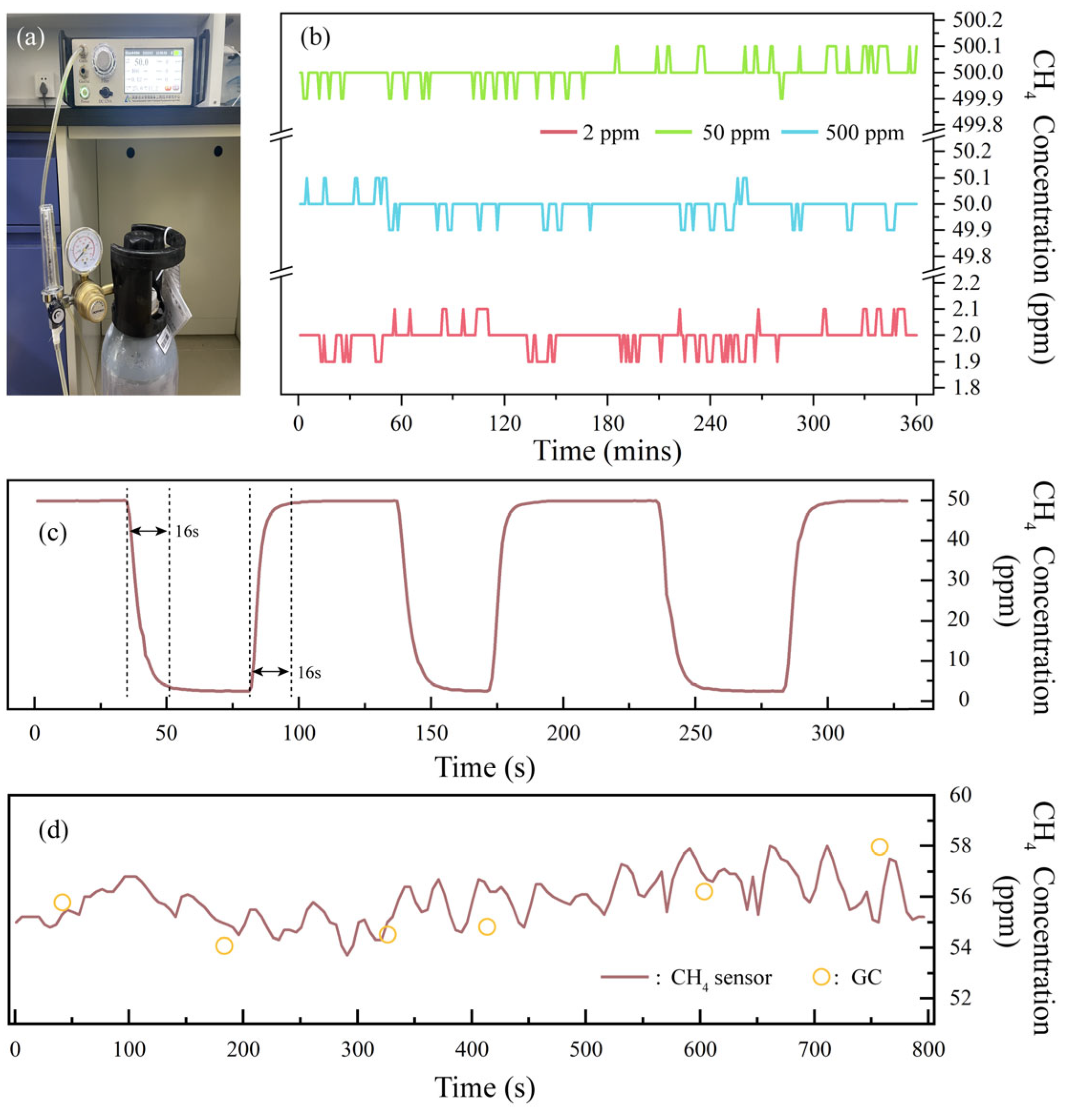
2.2. Monitoring System

The in situ continuous monitoring system used to study the sewage inspection wells includes a self-developed portable TDLAS CH₄ sensor and a thermosensitive gas velocity analyser (AR866A, Smart Sensor, Hong Kong, China). In the CH₄ sensor, according to the absorption characteristics of CH₄ in the HITRAN spectral database [46], we chose a tuneable laser with a centre wavelength of 1654 nm from Wuhan 69 Sensor Technology Co. (Wuhan, China). The change in scanning current determines the wavelength selection of the laser while the temperature controller keeps the temperature constant at 25 °C. To reduce the influence of noise, we superimposed the low-frequency (5 Hz) scanning sawtooth wave on the high-frequency (5 kHz) scanning sine wave to realise wavelength modulation; the weak signal can be obtained from background noise [47]. It is known from Lambert–Beer’s law [48] that the detection sensitivity is proportional to the optical path [49]. Based on the concept of a portable application, the absorption cell of the CH₄ sensor was built as an annular reflector with a diameter of 60 mm, a height of 10 mm, and an effective optical path of 5 m, and the volume of the air chamber is only 25 mL. The external gas entering the gas absorption cell through the “Gas In” port under the action of the built-in air pump attenuates the laser so that more accurate monitoring can be achieved. The photodetector we used is G10899-01K from Hamamatsu Photonics (Beijing, China) Co. Through concentration inversion, the lock-in amplifier demodulates the second harmonic signal, and the microcontroller STM32F103 collects the demodulated signal. A lock-in amplifier demodulates the second harmonic signal obtained by concentration inversion. The microcontroller model STM32F103 collects demodulated signals. In addition, our portable sensor also integrates the all-in-one sensor module PTQS1005A from Beijing Planttower Co., Ltd. (Beijing, China) to simultaneously monitor the gas temperature, with a temperature detection range of −10~55 °C and a resolution of 0.1 °C. The real-time data obtained from the measurement are transmitted to the mobile phone app through the Bluetooth module and stored automatically. We used standard gas to verify the accuracy of the portable TDLAS CH₄ sensor. The standard gas was purchased from Beijing Nanfei Gas Technology Development Co., Ltd. (Beijing, China), and the inaccuracy of the concentration value was less than 2%. At the same time, these standard gases were also used to calibrate the sensor before the field experiment. Moreover, we simultaneously collected gas samples for gas chromatography analysis to confirm the instrument’s accuracy in field monitoring. Specifically, we filled and cleaned the syringe three times, attached a hypodermic needle, extended the syringe into the well, collected the gas, and transferred the sample to a 12 mL pre-evacuated bottle. In the laboratory, a gas chromatograph (Agilent 7890-0468, Santa Clara, CA, USA) equipped with a flame ionisation detector (FID) and a microcell electron capture detector (ECD) was used to detect the CH₄ concentration of gas samples. The standard gas with a known CH₄ concentration and the collected gas samples were analysed to facilitate the instrument’s calibration.

The measurement range of the thermosensitive gas velocity analyser (Smart Sensor AR866A, Hong Kong, China) is 0–30 m/s, and the measurement accuracy is ±1%. The measuring range of air temperature is 0–45 °C, and the measuring accuracy is ±1 °C. The probe bracket can be bent and extended to 960 mm, which is convenient for measuring wind speed in various spaces. A thermosensitive chip was installed inside the probe; the external structure design of the probe with a one-way opening along the chip allows the sensor to better measure the gas flow rate in one direction. In practical applications, the probe is placed tightly above the vent hole to measure the gas flow velocity in the vertical direction (Figure 2c). The gas flow is due to the pressure difference between the inside and outside of the inspection well. Guisasola et al. [50] simulated a closed sewage pipe system in the laboratory and found that the pressure in the system was greater than that of external air. Hartley and Lant [51] also observed a similar phenomenon in their work, which showed that the continuous production of gas in the sewage inspection well increases the internal pressure of the well and causes the air in the well to be pushed out through the vent hole. At the same time, the wind blowing through the well’s outer surface will also affect the speed of air exchange. The real-time measurement data are stored directly in the analyser or connected to the laptop for storage.

2.3. Flux Calculation Method

The gas flux is determined by the concentration and flow velocity [22,26]. We calculated the flux based on theoretical knowledge of infrared thermometry using a portable TDLAS CH₄ sensor and a thermosensitive gas velocity analyser (Figure 2). Firstly, we connected the portable sensor’s “Gas In” port to a position about 1 cm inside the first vent hole on the sewage inspection well via a gas tube. Secondly, a long gas tube was connected to the portable sensor’s “Gas Out” port and deep into the first vent hole of the sewage inspection well, thus forming a gas circulation loop. Real-time monitoring of CH₄ concentration at a depth of about 1 cm in the vent hole of the sewage inspection well was thus achieved. The measured value was the CH₄ concentration of the gas exchanged between the sewage inspection well and the external environment. Finally, while measuring the concentration, we used a thermosensitive gas velocity analyser to monitor the vertical gas velocity on the surface of the second vent hole in the sewage inspection well.

The volume $V_{\mathrm{g}\mathrm{a}\mathrm{s}}$ (m³) of gas exchanged between the sewage inspection well and the external environment per unit of time can be obtained from the equation

$$V_{\mathrm{g}\mathrm{a}\mathrm{s}}=2S\times t\times v_{\mathrm{w}\mathrm{i}\mathrm{n}\mathrm{d}}$$

(1)

where $S$ (m³) is the area of a single vent hole of the sewage inspection well, calculated from the measured size and geometric relationship. The average total area of the two vent holes in each sewage inspection well is about 10.47 cm². $t$ (s) is the time, and $v_{\mathrm{w}\mathrm{i}\mathrm{n}\mathrm{d}}$ (m/s) is the wind speed measured using the gas velocity analyser.

The volume of CH₄ ($V_{{\mathrm{C}\mathrm{H}}_4}$) contained in the volume of gas exchanged per unit of time is

$$V_{{\mathrm{C}\mathrm{H}}_4}=V_{\mathrm{g}\mathrm{a}\mathrm{s}}\times C_{{\mathrm{C}\mathrm{H}}_4}$$

(2)

where $C_{{\mathrm{C}\mathrm{H}}_4}$ (m³) is the CH₄ concentration measured with the portable sensor.

Because the volume of the gas per unit of “amount of substance” varies at different temperatures [52], we can obtain the volume ($V_{\mathrm{a}\mathrm{c}\mathrm{t}}$) of the gas of 1 mol “amount of substance” at the temperature of the measurement position according to the ideal gas equation:

$$P{V}_{\mathrm{a}\mathrm{c}\mathrm{t}}=nRT$$

(3)

where $P$ (atm) is the atmospheric pressure, $V_{\mathrm{a}\mathrm{c}\mathrm{t}}$ (m³) is the gas volume of 1 mol “amount of substance” at the field temperature, $n$ (mol) is the amount of substance, and the constant $R$ is expressed in many forms, where the value is 0.08206 (L∙atm∙mol⁻¹∙K⁻¹) and $T$ (K) is the temperature. The $P$ is about one standard atmospheric pressure, and the change is small.

In summary, we can obtain the number of moles of CH₄ exchanged between the sewage inspection well and the external environment per unit of time through the equation

$$n_{{\mathrm{C}\mathrm{H}}_4}=V_{{\mathrm{C}\mathrm{H}}_4}/V_{\mathrm{a}\mathrm{c}\mathrm{t}}$$

(4)

When the time is 1 s, the CH₄ flux per second (mol/s) is numerically equal to the number of moles $n_{{\mathrm{C}\mathrm{H}}_4}$ (mol). To better quantify this, we can also further convert this value into the flux value in the standard temperature and pressure (STP) according to Equation (3).

2.4. Estimation Method of Total Urban CH₄ Exchange

We monitored the concentration of 56 sewage inspection wells in the study area for a long time. We selected a sewage inspection well and observed the continuous change in its concentration over five days. At the same time, the concentrations of 56 inspection wells were randomly measured and recorded, and the measurement time was randomly distributed at different periods of each day. The concentration of each sewage inspection well was the average value of multiple data. Based on these data, we drew the CH₄ concentration hot spot map of the inspection wells and estimated the average concentration of sewage inspection wells in the whole city. Then, combined with the average gas exchange velocity, the average exchange flux of CH₄ was obtained. Finally, according to information such as the length of the urban pipeline and the setting of inspection wells, the total number of inspection wells in the city was obtained, and the total amount of CH₄ exchange was calculated [30].

The facilities in the study area are common in cities, but the concentration data of the 56 sewage inspection wells may be non-normally distributed, and there may be uncertainty. In previous studies, the bootstrap method has been used to estimate the overall mean of similar datasets [45,53]. In our work, the initial sample set of the bootstrap method comprised M (M = 56) CH₄ sample concentrations. We then randomly extracted a sample from the initial sample set independently with equal probability, which was put back after taking it out, and repeated the process M times. These extracted samples constituted a new self-help sample set, and their average value $\theta$ was calculated. We repeatedly obtained a total of N (in our experiments, N = 2000) self-help sample sets, and the overall mean $\widehat{\theta }$ can be obtained through the equation

$$\widehat{\theta }=\left(1/N\right)\sum _{i=1}^N{\theta }_i$$

(5)

When estimating the overall mean of wind speed, three inspection wells were randomly selected and measured continuously for 10 min at a resolution of 1 s each time during the day and night for three days, and a total of 10,800 wind speed data were obtained. The “Lillietest” function verifies whether all the data have a normal distribution and whether the mean is calculated [54,55]. We combined the published “Beijing Water Affairs Statistical Yearbook” and other public information to obtain the total number of sewage inspection wells in the city to estimate the total mass of CH₄ exchange. We will also discuss the uncertainty of the data and compare them with existing related studies to verify our results.

3. Results and Discussion

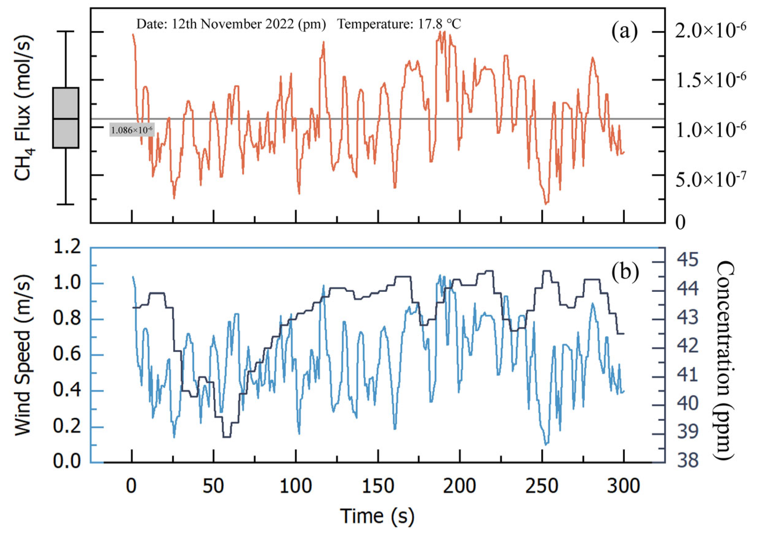
3.1. In Situ Continuous Monitoring of the Exchange Flux

We first demonstrated the accuracy and reliability of a portable CH₄ analyser for continuously monitoring in the field. We carried out 360 min of continuous monitoring (Figure 3a) of CH₄ standard gases with concentrations of 2 ppm, 50 ppm, and 500 ppm and found that the measurement results fluctuated within ±0.1 ppm of the concentration value declared by the manufacturer (Figure 3b). As determined via calculation according to the 3σ criterion, within 360 min, the detection accuracy of the standard gas with concentrations of 2 ppm, 50 ppm, and 500 ppm was 0.15 (3σ) ppm, 0.14 (3σ) ppm, and 0.16 (3σ) ppm, respectively. We also used 50 ppm CH₄ standard gas to show the sensor’s repeatability (Figure 3c). When the sensor stopped supplying the gas while continuously detecting the standard gas, it took only 16 s for the results to drop to an atmospheric average concentration of about 2.1 ppm and remain stable. Moreover, to ensure the accuracy of the results of on-site monitoring, we carried out a comparative experiment to synchronously collect gas samples for gas chromatographic analysis; this specific method was introduced in Section 2.2. It can be seen that at 800 s, the concentration trend of the six gas chromatography sampling points was the same as that in the continuous monitoring results, and the difference may be the error caused by the collection and transfer of samples or the inherent error of the system (Figure 3d). These results show the accuracy and stability of the CH₄ concentration analyser.

For in situ continuous flux monitoring, we randomly selected a sewage inspection well (No. 43 of 56) for monitoring. The gas exchange rate was recorded at a frequency of 1 s in 5 min, and the CH₄ concentration was recorded at 5 s. We can see that the wind speed in Figure 4b varied from 0.1 to 1.0 m/s, mainly due to the change in gas pressure inside and outside the sewage inspection well [19]; this includes the pressure rise caused by the continuous production of gas inside the well [50] and the pressure fluctuation caused by the wind blowing through the well’s outer surface. In the experiment, we also tried to place the probe of the analyser above the middle of the circular solid cover of the well, and the detected wind speed was almost zero. This shows that the analyser can more accurately measure the vertical flow rate of gas exchanged through the vent hole in our scenario. The CH₄ concentration in Figure 4b varied around 42 ppm, fluctuating from 38.5 to 44.5 ppm, and the degree of variation was about 14%. We compared our results with the work of Sun et al. [56]; they simulated a sewer system in the laboratory and collected headspace gas for gas chromatographic analysis. The results show that the CH₄ concentration had periodic fluctuations. Over 10 to 30 min, the degree of change was about 20–30%, indicating that the CH₄ concentration fluctuations demonstrated by our monitoring results are normal. The flux calculated based on the measured data reflects the rate of CH₄ exchange between the sewage inspection well and the atmosphere. It changed within 5 min (Figure 4a); the median value was about 1.086 × 10⁻⁶ mol/s. When the concentration was relatively small, the effect of wind speed on the flux was greater than that of the concentration.

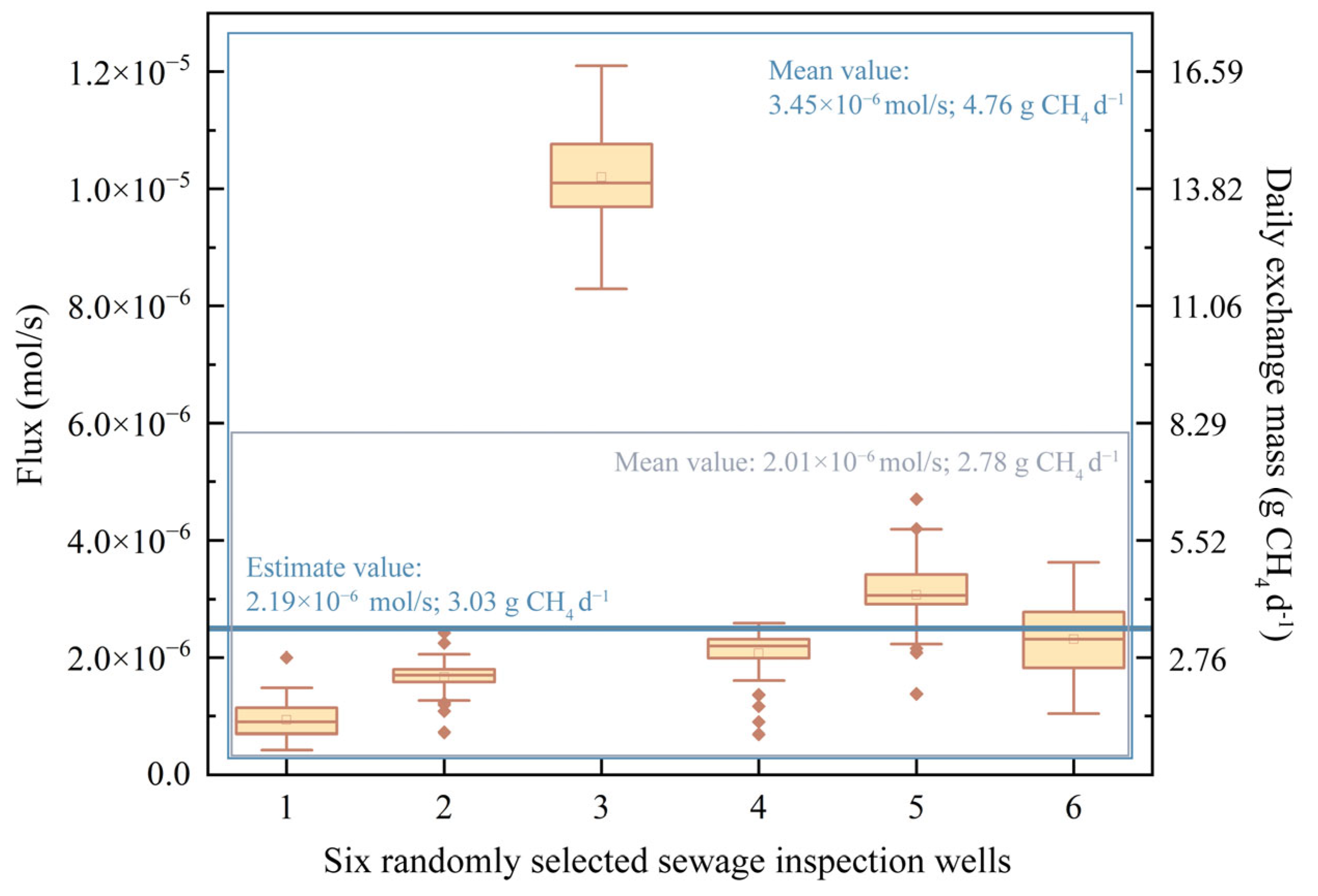
3.2. The Total Amount of CH₄ Exchange in Sewage Inspection Wells in the Whole City

With the development of urban modernisation, the number of sewage inspection wells continues to increase. According to public information from the Beijing Municipal Water Affairs Bureau’s Beijing Sewage Statistical Yearbook, as of 2020, the collective length of sewage pipelines in Beijing is about 14,920 km. Taking the CH₄ concentration information of sewage inspection wells in the research area as a sample, we estimated the annual total amount of CH₄ exchanged between sewage inspection wells and the atmosphere in Beijing.

We first randomly selected a sewage inspection well (No. 4 of 56) in the research area chosen for periodic monitoring to explore the characteristics of CH₄ exchange (Figure 5). For five consecutive days, monitoring was performed for 20 min in the morning, afternoon, and evening. The night of November 11, the morning of November 12, and the night of November 13 were not measured due to rainfall. Through observation, it was found that during three days, from 11.09 to 11.11 (Wednesday to Friday), the CH₄ concentration generally showed an upward trend, and a significant decline occurred from 11.12 to 11.13 (Saturday to Sunday).

The CH₄ concentration from Wednesday to Friday was higher than that on Saturday and Sunday (Figure 5a), which was possibly related to the rain that started on Friday night. Firstly, the rainfall led to a drop in temperature, and we analysed the correlation between CH₄ concentration and temperature. However, the data analysis results do not show a convincing connection between changes in CH₄ concentration and temperature. The Pearson correlation coefficient between them was 0.35, showing a weak correlation, and the adjusted r-squared of the regression analysis was only 0.22, which indicates that the quality of regression fitting is low; thus, the data point in the upper-right corner of Figure 5b has a great influence on the fitting quality. We believe more data and greater literature support are needed to demonstrate their relevance. Secondly, according to existing studies, we believe the large amount of water brought about by rainfall is the main factor leading to decreased CH₄ concentration. In their study, Sun et al. [56] found that more CH₄ was produced in a sewer network when water use was reduced than when water use was higher. In a simulated sewer system study, Guisasola et al. [50] found that the shorter the hydraulic retention time of sewage, the higher the CH₄ production. Rainwater will dilute the sewage in a pipe and accelerate the flow of sewage, which may be the driving factor of the decrease in CH₄ concentration, resulting in low CH₄ concentration on rest days.

Because of the time specificity of CH₄ concentration in sewage inspection wells, predicting CH₄ exchange over a long duration is relatively difficult. In estimating the total amount of CH₄ exchanged between sewage inspection wells and the atmosphere in Beijing in the autumn (August–October) of 2022, we first monitored the CH₄ concentration in 56 sewage inspection wells in the research area and took this as a sample. The experiment was carried out from August to October, and the measurement time was randomly distributed at different periods of each day. The concentration of each sewage inspection well was the average value of multiple data, and a hot spot map was drawn, as shown in Figure 6a.

The CH₄ concentration of the samples showed a non-normal distribution; we used the bootstrap method introduced in Materials and Methods to calculate the average concentration of 102.5 ppm in all inspection wells. Shah et al. [29] monitored the CH₄ concentration in a wet well for two days by collecting gas samples and using gas chromatography analysis, and the average concentration was 116 ppm. Although the target they chose is not exactly the same as ours in terms of external factors such as region, it still shows that our estimation results are relatively reasonable. The 10,800 data from the wind speed monitoring were verified by the “Lillietest” function to be normally distributed; the expected Avg was 0.496 m/s, and the standard deviation was 0.146 (Figure 6b). Combined with the average temperature of 22 °C during the measurement period, we estimate that the average CH₄ exchange flux of a single sewage inspection well is 2.19 × 10⁻⁶ mol/s, and based on the molar mass of CH₄, the daily amount of CH₄ exchanged in a sewage inspection well is 3.03 g CH₄ d⁻¹.

We compared the estimated results with the monitoring data of six randomly selected sewage inspection wells (Figure 7). This part of the supplementary experiment was conducted in August 2023. The analysis found that the average exchange flux of five wells was 2.01 × 10⁻⁶ mol/s, and the daily exchange mass was 2.78 g CH₄ d⁻¹, which is very close to our estimated results. However, the value of the third well was higher, which is quite different from our estimated results. We believe this is a normal phenomenon; this difference will decrease with an increase in samples. We used the “bootstrap” method to estimate the overall mean in our study to reduce the impact of this phenomenon on the results, and we will conduct more sampling procedures and analyses in future studies.

In another study, Lamb et al. [57] reported that the average emission rate of natural gas distribution main leakage in the United States ranges from 432 to 1728 g CH₄ d⁻¹, much higher than our estimated CH₄ exchange rate of 3.03 g CH₄ d⁻¹. This difference may be because our research focused only on sewage inspection wells rather than natural gas pipelines. In contrast, Hendrick et al. [58] monitored CH₄ hot spots in the city of Boston, targeting CH₄ sources such as sewage inspection wells, natural gas pipeline leaks, roadway drill holes, and urban greenspaces, and obtained CH₄ emission fluxes in the range of 4.0 to 2.3 × 10⁴ g CH₄ d⁻¹. The CH₄ concentration of sewage inspection wells was lower than that of other CH₄ sources, and the initial value of the flux range in their results was 4.0 g CH₄ d⁻¹, which is close to our estimated CH₄ flux of 3.03 g CH₄ d⁻¹. Considering the previous differences in each city, our prediction result is credible.

The overall emissions can be obtained according to the number of inspection wells in the city and the average emission flux [30]. The concept of “per capita sewerage network length” is mentioned in Von Sperling’s book Wastewater Characteristics, Treatment and Disposal [59], which explains that the design and construction of sewage networks are related to city size and regional population density. So, we can reasonably infer that urban central areas have high population density and large sewage discharge, corresponding to a longer length of sewage pipes, and vice versa. This design and construction method reduces the differences between sewage pipes in different urban areas, and it also shows that although there were errors in how we estimated the total CH₄ emissions based on the total length of urban sewage pipes, our results are also relatively reasonable. As mentioned earlier, the total length of sewage pipes in Beijing was about 14,920 km in 2020. In municipal engineering, the distance between sewage inspection wells is related to the pipeline’s diameter. It is usually required to be at most 30 m in actual construction, and it can be estimated that there are about 497,333 sewage inspection wells. From this, we can conservatively infer that the sewage inspection wells in Beijing exchanged at least 8.47 × 10⁶ mol CH₄ with the atmosphere in the autumn of 2022 (about 1.35 × 10⁵ kg), and the total amount over the whole year is about 5.49 × 10⁵ kg CH₄ yr⁻¹. As a potential source of CH₄, sewage inspection wells are often overlooked, even in wastewater treatment studies, and the CH₄ emissions published in greenhouse gas inventories usually do not include their contribution, even though it may account for only a small portion [15]. The Emissions Database for Global Atmospheric Research (EDGAR) collects information on man-made greenhouse gas emissions and air pollution on Earth [60]. In its latest data, the CH₄ emissions from China in the autumn of 2021 total about 1.89 × 10⁴ kt, and the total CH₄ emissions over the whole year reach 7.1 × 10⁴ kt. CH₄ comes from agriculture, manufacturing, and other sectors. Although the total amount of CH₄ exchanged between sewage inspection wells and the atmosphere is low, it is still essential to accurately evaluate and include it in the greenhouse gas inventories.

4. Conclusions

This study shows that sewage inspection wells are a potential source of CH₄. We propose a method for in situ continuous monitoring of sewage inspection wells and atmospheric exchange CH₄ flux. Compared with other detection methods, such as gas chromatography and optical cavity ring-down spectroscopy, TDLAS has a slightly lower quantitative accuracy. Still, it has the advantages of a low cost and simple operation. We used a self-developed portable TDLAS CH₄ sensor and a gas velocity analyser to achieve flux monitoring. The fluctuation range of the sensor when monitoring the standard gas is ±0.1 ppm of the target concentration. Relevant theoretical knowledge of infrared thermometry was used to calibrate the effect of temperature on the results. We took 56 sewage inspection wells in the research area as a small sample set and obtained the average concentration of urban sewage inspection wells during the experiment using the bootstrap method, which amounted to about 102.5 ppm; combined with the average gas velocity measured during monitoring of 0.496 m/s, it is estimated that the CH₄ exchange flux between sewage inspection wells and the atmosphere is about 3.03 g CH₄ d⁻¹. The annual CH₄ exchange mass of urban sewage inspection wells is about 5.49 × 10⁵ kg CH₄ yr⁻¹. The accuracy of the results was verified by synchronous analysis of gas chromatography and comparison with other work.

However, the proposed method still has some limitations and shortcomings. For example, rainfall, snow, storms, and other weather may impact in situ monitoring. Therefore, the monitoring method is suitable for most seasons as long as these special weather conditions are avoided. At the same time, when evaluating the total amount of CH₄ exchanged with the atmosphere by sewage inspection wells in the whole city, because the samples in the selected research area cannot completely and accurately represent the whole city, even though the design and construction of sewer pipes will take into account information such as population density in different urban areas, there will still be potential errors in the results. Sampling monitoring in a larger area would lead to more accurate results.

We will further optimise the CH₄ sensor’s performance in future work by using a larger optical path absorption cell and a more effective noise reduction method. We will also expand the research area and collect more monitoring data to improve the accuracy of the estimation results. Other methods can also monitor the CH₄ flux of sewage inspection wells, and we should consider comparing experimental results with them. For example, the static gas chamber method is more commonly used. It requires a closed gas chamber at the wellhead, and the flux is obtained by connecting the online concentration detection instrument or transferring gases to the laboratory after sampling. The IFTS method mentioned earlier can simultaneously obtain each pixel’s spatial position and spectral information in the field of vision and calculate the CH₄ flux through continuous imaging. We should also focus on characterising the temporal and spatial changes in CH₄ concentration in more detail, focusing on daily and monthly changes, and understanding the effects of water level and microbial content changes in sewers on the CH₄ flux. These efforts will provide a reference for improving the greenhouse gas inventory and designating measures for climate change. This study will help deal with climate change, improve existing atmospheric emission databases and models, and contribute to environmental protection.

References

1. Intergovernmental Panel on Climate Change. Climate Change 2014: Synthesis Report. Available online: https://www.ipcc.ch/site/assets/uploads/2018/05/SYR_AR5_FINAL_full_wcover.pdf (accessed on 18 October 2023).
2. Wuebbles, D.J.; Hayhoe, K. Atmospheric Methane and Global Change. Earth Sci. Rev. 2002, 57, 177–210. [Google Scholar] [CrossRef]
3. Hou, R.; Li, T.; Fu, Q.; Liu, D.; Li, M.; Zhou, Z.; Li, L.; Yan, J. Characteristics of Water–heat Variation and the Transfer Relationship in Sandy Loam under Different Conditions. Geoderma 2019, 340, 259–268. [Google Scholar] [CrossRef]
4. Zhang, T.; Wu, S.; Fang, X.; Han, Z.; Li, S.; Wang, J.; Liu, S.; Zou, J. Spatiotemporal Variations of Dissolved CH4 Concentrations and Fluxes from Typical Freshwater Types in An Agricultural Irrigation Watershed in Eastern China. Environ. Pollut. 2022, 314, 120246. [Google Scholar] [CrossRef] [PubMed]
5. Yamaji, K.; Ohara, T.; Akimoto, H. Regional-specific emission inventory for NH3, N2O, and CH4 via animal farming in South, Southeast, and East Asia. Atmos. Environ. 2004, 38, 7111–7121. [Google Scholar] [CrossRef]
6. Zhu, T.; Bian, W.; Zhang, S.; Di, P.; Nie, B. An Improved Approach to Estimate Methane Emissions from Coal Mining in China. Environ. Sci. Technol. 2017, 51, 12072–12080. [Google Scholar] [CrossRef] [PubMed]
7. Hu, N.; Liu, S.; Gao, Y.; Xu, J.; Zhang, X.; Zhang, Z.; Lee, X. Large Methane Emissions from Natural Gas Vehicles in Chinese Cities. Atmos. Environ. 2018, 187, 374–380. [Google Scholar] [CrossRef]
8. Wang, J.; Li, Y.; Zhang, Y. Research on Carbon Emissions of Road Traffic in Chengdu City Based on A LEAP Model. Sustainability 2022, 14, 5625. [Google Scholar] [CrossRef]
9. Wu, H.; Dong, L.; Yin, X.; Sampaolo, A.; Patimisco, P.; Ma, W.; Zhang, L.; Yin, W.; Xiao, L.; Spagnolo, V.; et al. Atmospheric CH4 Measurement Near A Landfill Using an ICL-based QEPAS Sensor with V-T Relaxation Self-calibration. Sens. Actuators B Chem. 2019, 297, 126753. [Google Scholar] [CrossRef]
10. Masuda, S.; Suzuki, S.; Sano, I.; Li, Y.-Y.; Nishimura, O. The Seasonal Variation of Emission of Greenhouse Gases from A Full-scale Sewage Treatment Plant. Chemosphere 2015, 140, 167–173. [Google Scholar] [CrossRef]
11. Gålfalk, M.; Påledal, S.N.; Sehlén, R.; Bastviken, D. Ground-based Remote Sensing of CH4 and N2O Fluxes from A Wastewater Treatment Plant and Nearby Biogas Production with Discoveries of Unexpected Sources. Environ. Res. 2022, 204, 111978. [Google Scholar] [CrossRef]
12. Lu, L.; Li, X.; Li, Z.; Chen, Y.; Sabio-y-García, C.A.; Yang, J.; Luo, F.; Zou, X. Aerobic methanotrophs in an urban water cycle system: Community structure and network interaction pattern. Sci. Total Environ. 2021, 772, 145045. [Google Scholar] [CrossRef] [PubMed]
13. Mulder, K. Future Options for Sewage and Drainage Systems Three Scenarios for Transitions and Continuity. Sustainability 2019, 11, 1383. [Google Scholar] [CrossRef]
14. Lv, P.; Zhang, J.; Pang, L.; Yang, K.; Sun, S. Influence of Multiple Factors on the Explosion Characteristics of Flammable Gases in Municipal Sewage Pipelines. Adv. Civ. Eng. 2020, 2020, 3193012. [Google Scholar] [CrossRef]
15. Eijo-Río, E.; Petit-Boix, A.; Villalba, G.; Suárez-Ojeda, M.E.; Marin, D.; Amores, M.J.; Aldea, X.; Rieradevall, J.; Gabarrell, X. Municipal sewer networks as sources of nitrous oxide, methane and hydrogen sulphide emissions: A review and case studies. J. Environ. Chem. Eng. 2015, 3, 2084–2094. [Google Scholar] [CrossRef]
16. Fernandez, J.M.; Maazallahi, H.; France, J.L.; Menoud, M.; Corbu, M.; Ardelean, M.; Calcan, A.; Townsend-Small, A.; van der Veen, C.; Fisher, R.E.; et al. Street-level Methane Emissions of Bucharest, Romania and the Dominance of Urban Wastewater. Atmos. Environ. X 2022, 13, 100153. [Google Scholar] [CrossRef]
17. Phillips, N.G.; Ackley, R.; Crosson, E.R.; Down, A.; Hutyra, L.R.; Brondfield, M.; Karr, J.D.; Zhao, K.; Jackson, R.B. Mapping Urban Pipeline Leaks: Methane Leaks Across Boston. Environ. Pollut. 2013, 173, 1–4. [Google Scholar] [CrossRef]
18. Gålfalk, M.; Olofsson, G.; Bastviken, D.; Yamaji, K. Approaches for Hyperspectral Remote Flux Quantification and Visualization of GHGs in the Environment. Remote Sens. Environ. 2017, 191, 81–94. [Google Scholar] [CrossRef]
19. Maier, M.; Weber, T.K.D.; Fiedler, J.; Fuß, R.; Glatzel, S.; Huth, V.; Jordan, S.; Jurasinski, G.; Kutzbach, L.; Schäfer, K.; et al. Introduction of A Guideline for Measurements of Greenhouse Gas Fluxes from Soils Using Non-steady-state Chambers. J. Plant Nutr. Soil Sci. 2022, 185, 447–461. [Google Scholar] [CrossRef]
20. Williams, J.P.; El Hachem, K.; Kang, M. Controlled-release Testing of The Static Chamber Methodology for Direct Measurements of Methane Emissions. Atmos. Meas. Tech. Discuss. 2023, 16, 3421–3435. [Google Scholar] [CrossRef]
21. Zhao, J.; Zhang, M.; Xiao, W.; Wang, W.; Zhang, Z.; Yu, Z.; Xiao, Q.; Cao, Z.; Xu, J.; Zhang, X.; et al. An Evaluation of The Flux-gradient and The Eddy Covariance Method to Measure CH4, CO2, and H2O Fluxes from Small Ponds. Agric. For. Meteorol. 2019, 275, 255–264. [Google Scholar] [CrossRef]
22. Gålfalk, M.; Bastviken, M. Remote Sensing of Methane and Nitrous Oxide Fluxes from Waste Incineration. Waste Manag. 2018, 75, 319–326. [Google Scholar] [CrossRef] [PubMed]
23. Engram, M.; Anthony, K.W.; Sachs, T.; Kohnert, K.; Serafimovich, A.; Grosse, G.; Meyer, F. Remote Sensing Northern Lake Methane Ebullition. Nat. Clim. Chang. 2020, 10, 511–517. [Google Scholar] [CrossRef]
24. Zhu, Y.; Merbold, L.; Leitner, S.; Wolf, B.; Pelster, D.; Goopy, J.; Butterbach-Bahl, K. Interactive Effects of Dung Deposited onto Urine Patches on Greenhouse Gas Fluxes from Tropical Pastures in Kenya. Sci. Total Environ. 2021, 761, 143184. [Google Scholar] [CrossRef]
25. Wang, W.; Sardans, J.; Wang, C.; Zeng, C.; Tong, C.; Asensio, D.; Penuelas, J. Relationships Between the Potential Production of the Greenhouse Gases CO2, CH4 and N2O and Soil Concentrations of C, N and P Across 26 Paddy Fields in Southeastern China. Atmos. Environ. 2017, 164, 458–467. [Google Scholar] [CrossRef]
26. Tang, A.C.I.; Stoy, P.C.; Hirata, R.; Musin, K.K.; Aeries, E.B.; Wenceslaus, J.; Melling, L. Eddy Covariance Measurements of Methane Flux at A Tropical Peat Forest in Sarawak, Malaysian Borneo. Geophys. Res. Lett. 2018, 45, 4390–4399. [Google Scholar] [CrossRef]
27. Lauvaux, T.; Giron, C.; Mazzolini, M.; d’Aspremont, A.; Duren, R.; Cusworth, D.; Shindell, D.; Ciais, P. Global Assessment of Oil and Gas Methane Ultra-emitters. Science 2022, 375, 557–561. [Google Scholar] [CrossRef] [PubMed]
28. Krommweh, M.S.; Schmithausen, A.J.; Deeken, H.F.; Büscher, W.; Maack, G.-C. A New Experimental Setup for Measuring Greenhouse Gas and Volatile Organic Compound Emissions of Silage During the Aerobic Storage Period in A Special Silage Respiration Chamber. Environ. Pollut. 2020, 257, 115513. [Google Scholar] [CrossRef]
29. Shah, A.; Willis, J.; Fillmore, L. Quantifying Methane Evolution from Sewers: Results from WERF/Dekalb phase 2 Continuous Monitoring at Honey Creek Pumping Station and Force Main. In Proceedings of the Water Environment Federation, Raleigh, NC, USA, 12–15 June 2011; Water Environment Federation: Alexandria, VA, USA, 2011; pp. 475–485. [Google Scholar]
30. Fries, A.E.; Schifman, L.A.; Shuster, W.D.; Townsend-Small, A. Street-level Emissions of Methane and Nitrous Xxide from the Wastewater Collection System in Cincinnati, Ohio. Environ. Pollut. 2018, 236, 247–256. [Google Scholar] [CrossRef]
31. Zhang, L.; Song, L.; Wang, B.; Shao, H.; Zhang, L.; Qin, X. Co-effects of Salinity and Moisture on CO2 and N2O Emissions of Laboratory-incubated Salt-affected Soils from Different Vegetation Types. Geoderma 2018, 332, 109–120. [Google Scholar] [CrossRef]
32. Zhang, G.; Xiao, X.; Dong, J.; Xin, F.; Zhang, Y.; Qin, Y.; Doughty, R.B.; Moore, B. Fingerprint of Rice Paddies in Spatial–temporal Dynamics of Atmospheric Methane Concentration in Monsoon Asia. Nat. Commun. 2020, 11, 554. [Google Scholar] [CrossRef]
33. Wang, Y.; Zhang, Y.; Zhao, C.; Dong, D.; Wang, K. CO and CH4 Atmospheric Trends from Dense Multi-point Forest Fires Around the City of Chongqing using Spaceborne Spectrometer Data. Atmos. Pollut. Res. 2023, 14, 101807. [Google Scholar] [CrossRef]
34. Fu, B.; Zhang, C.; Lyu, W.; Sun, J.; Shang, C.; Cheng, Y.; Xu, L. Recent Progress on Laser Absorption Spectroscopy for Determination of Gaseous Chemical Species. Appl. Spectrosc. Rev. 2022, 57, 112–152. [Google Scholar] [CrossRef]
35. Li, J.; Yu, Z.; Du, Z.; Ji, Y.; Liu, C. Standoff Chemical Detection Using Laser Absorption Spectroscopy: A Review. Remote Sens. 2020, 12, 2771. [Google Scholar] [CrossRef]
36. Witzel, O.; Klein, A.; Meffert, C.; Wagner, S.; Kaiser, S.; Schulz, C.; Ebert, V. VCSEL-based, High-speed, in situ TDLAS for In-cylinder Water Vapor Measurements in IC Engines. Opt. Express 2013, 21, 19951–19965. [Google Scholar] [CrossRef] [PubMed]
37. Jiao, L.; Dong, D.; Han, P.; Zhao, X.; Du, X. Identification of the Mango Maturity Level by the Analysis of Volatiles Based on Long Optical-path FTIR Spectroscopy and A Molecular Sieve. Anal. Methods 2017, 9, 2458–2463. [Google Scholar] [CrossRef]
38. Zhang, Y.; Nie, Y.; Liu, Y.; Huang, X.; Yang, Y.; Xiong, H.; Zhu, H.; Li, Y. Characteristics of Greenhouse Gas Emissions from Yellow Paddy Soils under Long-Term Organic Fertilizer Application. Sustainability 2022, 14, 12574. [Google Scholar] [CrossRef]
39. Machacova, K.; Vainio, E.; Urban, O.; Pihlatie, M. Seasonal dynamics of Stem N2O Exchange Follow the Physiological Activity of Boreal Trees. Nat. Commun. 2019, 10, 4989. [Google Scholar] [CrossRef]
40. Tirol-Padre, A.; Rai, M.; Gathala, M.; Sharma, S.; Kumar, V.; Sharma, P.C.; Sharma, D.K.; Wassmann, R.; Ladha, J. Assessing the Performance of the Photo-acoustic Infrared Gas Monitor for Measuring CO2, N2O, and CH4 Fluxes in Two Major Cereal Rotations. Glob. Change Biol. 2014, 20, 287–299. [Google Scholar] [CrossRef]
41. Guo, Y.; Qiu, X.; Li, N.; Feng, S.; Cheng, T.; Liu, Q.; He, Q.; Kan, R.; Yang, H.; Li, C. A Portable Laser-based Sensor for Detecting H2S in Domestic Natural Gas. Infrared Phys. Technol. 2020, 105, 103153. [Google Scholar] [CrossRef]
42. Jońca, J.; Pawnuk, M.; Bezyk, Y.; Arsen, A.; Sówka, I. Drone-Assisted Monitoring of Atmospheric Pollution-A Comprehensive Review. Sustainability 2022, 14, 11516. [Google Scholar] [CrossRef]
43. Dong, D.; Jiao, L.; Li, C.; Zhao, C. Rapid and Real-time Analysis of Volatile Compounds Released from Food Using Infrared and Laser Spectroscopy. Trends Analyt. Chem. 2019, 110, 410–416. [Google Scholar] [CrossRef]
44. Wang, K.; Guo, R.; Zhou, Y.; Jiao, L.; Dong, D. Detection of NH3 in Poultry Housing Based on Tunable Diode Laser Absorption Spectroscopy Combined with A Micro Circular Absorption Cell. Front. Phys. 2022, 10, 1051719. [Google Scholar] [CrossRef]
45. Efron, B.; Tibshirani, R. Bootstrap Methods for Standard Errors, Confidence Intervals, and Other Measures of Statistical Accuracy. Stat. Sci. 1986, 1, 54–75. [Google Scholar] [CrossRef]
46. Rothman, L.S.; Gordon, I.E.; Babikov, Y.; Barbe, A.; Benner, D.C.; Bernath, P.F.; Birk, M.; Bizzocchi, L.; Boudon, V.; Brown, L.R.; et al. The HITRAN 2012 Molecular Spectroscopic Database. J. Quant. Spectrosc. Radiat. Transf. 2013, 130, 4–50. [Google Scholar] [CrossRef]
47. Schilt, S.; Thévenaz, L.; Robert, P. Wavelength Modulation Spectroscopy: Combined Frequency and Intensity Laser Modulation. Appl. Opt. 2003, 42, 6728–6738. [Google Scholar] [CrossRef] [PubMed]
48. Lin, S.; Chang, J.; Sun, J.; Xu, P. Improvement of the Detection Sensitivity for Tunable Diode Laser Absorption Spectroscopy: A Review. Front. Phys. 2022, 10, 853966. [Google Scholar] [CrossRef]
49. Mangold, M.; Tuzson, B.; Hundt, M.; Jágerská, J.; Looser, H.; Emmenegger, L. Circular Paraboloid Reflection Cell for Laser Spectroscopic Trace Gas Analysis. J. Opt. Soc. Am. 2016, 33, 913–919. [Google Scholar] [CrossRef]
50. Guisasola, A.; de Haas, D.; Keller, J.; Yuan, Z. Methane Formation in Sewer Systems. Water Res. 2008, 42, 1421–1430. [Google Scholar] [CrossRef]
51. Hartley, K.; Lant, P. Eliminating Non-renewable CO2 Emissions from Sewage Treatment: An Anaerobic Migrating Bed Reactor Pilot Plant Study. Biotechnol. Bioeng. 2006, 95, 384–398. [Google Scholar] [CrossRef]
52. Tenny, K.M.; Cooper, J.S. Ideal Gas Behavior; StatPearls Publishing: Treasure Island, FL, USA, 2017. [Google Scholar]
53. Jhun, M.; Jeong, H.-C. Applications of Bootstrap Methods for Categorical Data Analysis. Comput. Stat. Data Anal. 2000, 35, 83–91. [Google Scholar] [CrossRef]
54. Kallistova, A.Y.; Sabrekov, A.F.; Goncharov, V.M.; Pimenov, N.V.; Glagolev, M.V. On the Application of Statistical Analysis for Interpretation of Experimental Results in Environmental Microbiology. Microbiology 2019, 88, 232–239. [Google Scholar] [CrossRef]
55. Wang, J.; Ma, C.; Wang, S.; Lu, X.; Li, D. Risk Assessment Model and Sensitivity Analysis of Ordinary Arterial Highways Based on RSR–CRITIC–LVSSM–EFAST. Sustainability 2022, 14, 16096. [Google Scholar] [CrossRef]
56. Sun, J.; Hu, S.; Sharma, K.R.; Bustamante, H.; Yuan, Z. Impact of Reduced Water Consumption on Sulfide and Methane Production in Rising Main Sewers. J. Environ. Manag. 2015, 154, 307–315. [Google Scholar] [CrossRef]
57. Lamb, B.K.; Edburg, S.L.; Ferrara, T.W.; Howard, T.; Harrison, M.R.; Kolb, C.E.; Townsend-Small, A.; Dyck, W.; Possolo, A.; Whetstone, J.R. Direct Measurements Show Decreasing Methane Emissions from Natural Gas Local Distribution Systems in the United States. Environ. Sci. Technol. 2015, 49, 5161–5169. [Google Scholar] [CrossRef] [PubMed]
58. Hendrick, M.F.; Ackley, R.; Sanaie-Movahed, B.; Tang, X.; Phillips, N.G. Fugitive Methane Emissions from Leak-prone Natural Gas Distribution Infrastructure in Urban Environments. Environ. Pollut. 2016, 213, 710–716. [Google Scholar] [CrossRef] [PubMed]
59. Von Sperling, M. Wastewater Characteristics, Treatment and Disposal; IWA Publishing: London, UK, 2007. [Google Scholar]
60. Crippa, M.; Solazzo, E.; Huang, G.; Guizzardi, D.; Koffi, E.; Muntean, M.; Schieberle, C.; Friedrich, R.; Janssens-Maenhout, G. High Resolution Temporal Profiles in the Emissions Database for Global Atmospheric Research. Sci. Data 2020, 7, 121. [Google Scholar] [CrossRef]
Figure 1. Research location. Fifty-six sewage inspection wells are distributed in this area. We numbered these inspection wells and marked them according to their actual location.
Sustainability 15 16637 g001
Figure 2. Flux measurement system. (a) CH4 produced in the sewage inspection well is exchanged with the atmosphere through vent holes. (b) Schematic diagram of field measurement. (c) Monitoring schematic diagram.
Sustainability 15 16637 g002
Figure 3. Measurement accuracy and stability of TDLAS CH4 analyser. (a) Photo diagram for measuring CH4 standard gas. (b) Monitoring data for 2 ppm, 50 ppm, and 500 ppm concentrations of standard gases within 360 min. (c) Repeatability test of the sensor based on the standard gas. (d) Comparison of results from field monitoring and gas chromatography.
Sustainability 15 16637 g003
Figure 4. CH4 exchange flux monitoring of the sewage inspection well, the change in the CH4 flux between the inspection well and atmosphere within 5 min (a) was obtained according to the real-time recorded wind speed and CH4 concentration (b). The left boxplot in (a) illustrates the dispersion of the data, with the horizontal line in the middle indicating the location of the median.
Sustainability 15 16637 g004
Figure 5. Continuous monitoring experiment. CH4 concentrations and temperatures were recorded for five consecutive days at three different times daily (a), and a weak correlation was found between the two parameters (b). The dots in (b) correspond to the temperature and concentration of the monitoring data, and the line shows the results of fitting.
Sustainability 15 16637 g005
Figure 6. Hot spot map of CH4 concentration in sewage inspection wells (a) and normal fitting of gas flow velocity (b). The blue rectangle in (b) shows the data distribution, while the red line represents the fitting result.
Sustainability 15 16637 g006
Figure 7. The field monitoring results of six randomly selected wells compared with the estimated result based on the mean.
Sustainability 15 16637 g007
Disclaimer/Publisher’s Note: The statements, opinions and data contained in all publications are solely those of the individual author(s) and contributor(s) and not of MDPI and/or the editor(s). MDPI and/or the editor(s) disclaim responsibility for any injury to people or property resulting from any ideas, methods, instructions or products referred to in the content.