
A Hybrid Model of Variational Mode Decomposition and Long Short-Term Memory for Next-Hour Wind Speed Forecasting in a Hot Desert Climate


Abstract
:1. Introduction
- Proposing a novel hybrid model of the VMD method and LSTM model for next-hour WS prediction in a hot desert climate. This is the first work, to our knowledge, proposing a hybrid model for this combination of task and weather.
- Identifying the most important dataset features and the most suitable ML models for three climates: hot desert, humid continental and tropical. This is achieved through a performance comparison of the proposed model and two hybrid models of data decomposition techniques and the LSTM model, six DL-based models and four ML-based models, using previous hours’ WS values only versus using weather variables besides WS values.
- Measuring the performance gain of the proposed hybrid model over benchmark models to justify the added complexity and help make an informed decision on the tradeoff between accuracy and efficiency.
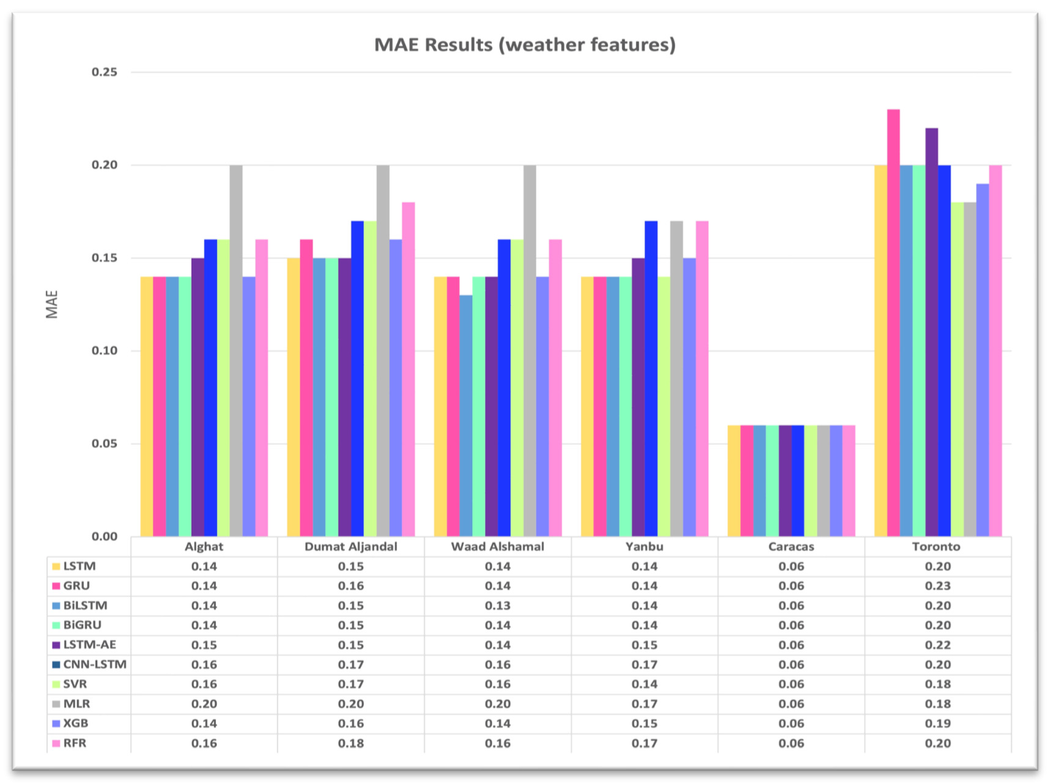
- Providing the forecasting results for four different locations in Saudi Arabia and two international locations, Caracas and Toronto. The results are presented using visualization and several performance metrics, including MAE, RMSE, MAPE and FS.
2. Related Work
Research Gap
3. Methodology
3.1. Data Preprocessing
3.1.1. Data Collection
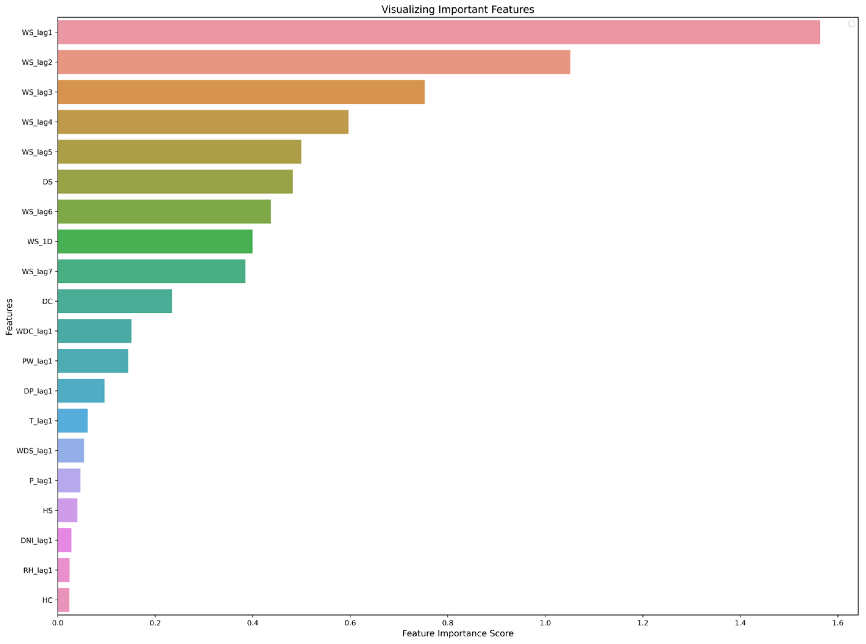
3.1.2. Feature Engineering
- Output: WS in meters per second (m/s);
- WD in degrees (°);
- Clear-sky GHI in watts per square meter (w/m2);
- Clear-sky DHI in w/m2;
- Clear-sky DNI in w/m2;
- Precipitable Water (PW) in millimeters;
- T in Celsius (°C);
- Dew Point (DP) in Celsius (°C);
- P in millibars;
- RH as a percentage (%).
3.1.3. Data Normalization and Portioning
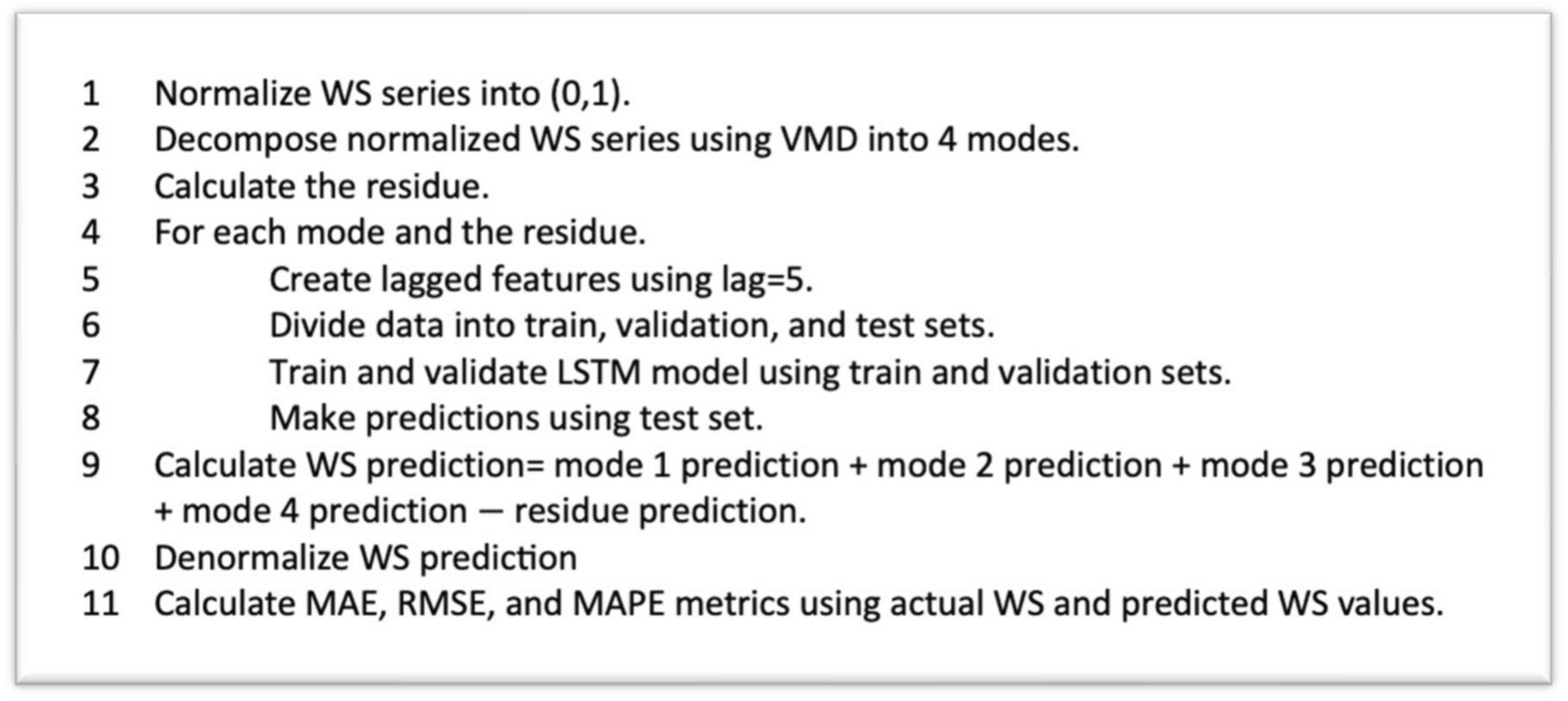
3.1.4. Data Decomposition Methods
EMD
CEEMDAN
VMD
3.2. Models’ Development
3.2.1. DL-Based Models
LSTM
GRU
BiLSTM
BiGRU
LSTM-AE
CNN-LSTM
Hybrid Model of Decomposition Methods and LSTM
3.2.2. ML-Based Models
SVR
RFR
XGB
MLR
3.3. Implementation
3.4. Evaluation Metrics
4. Results and Discussion
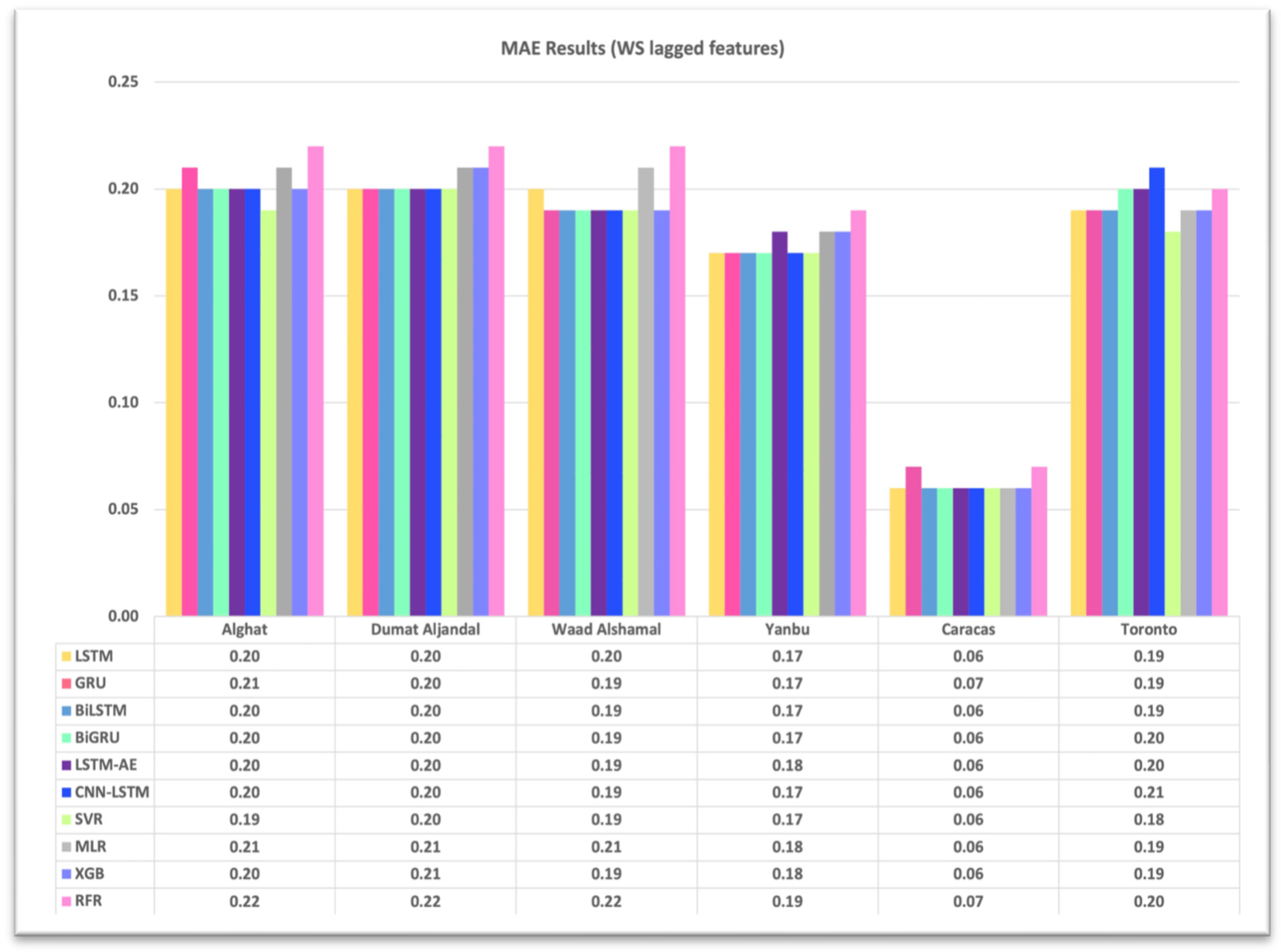
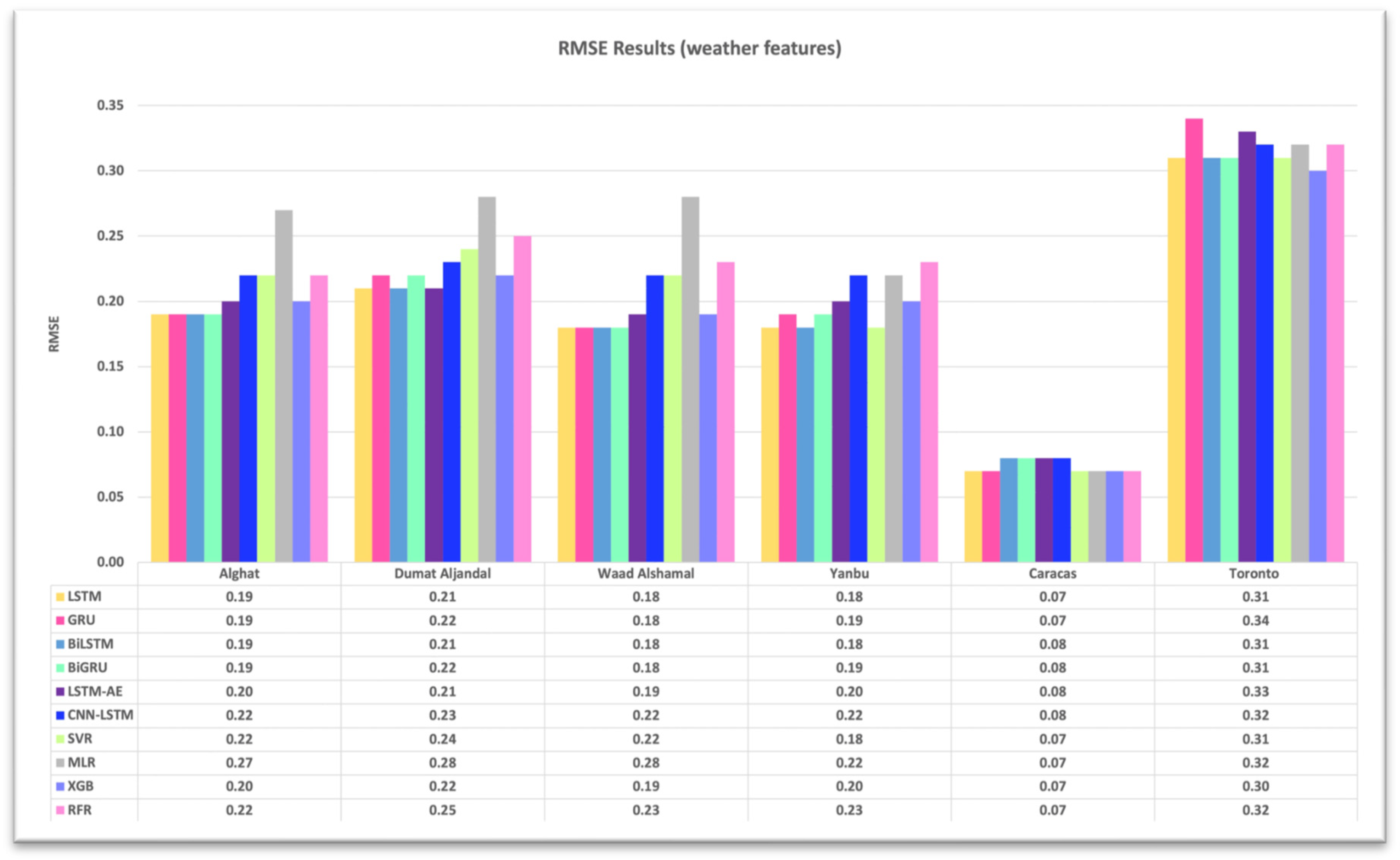
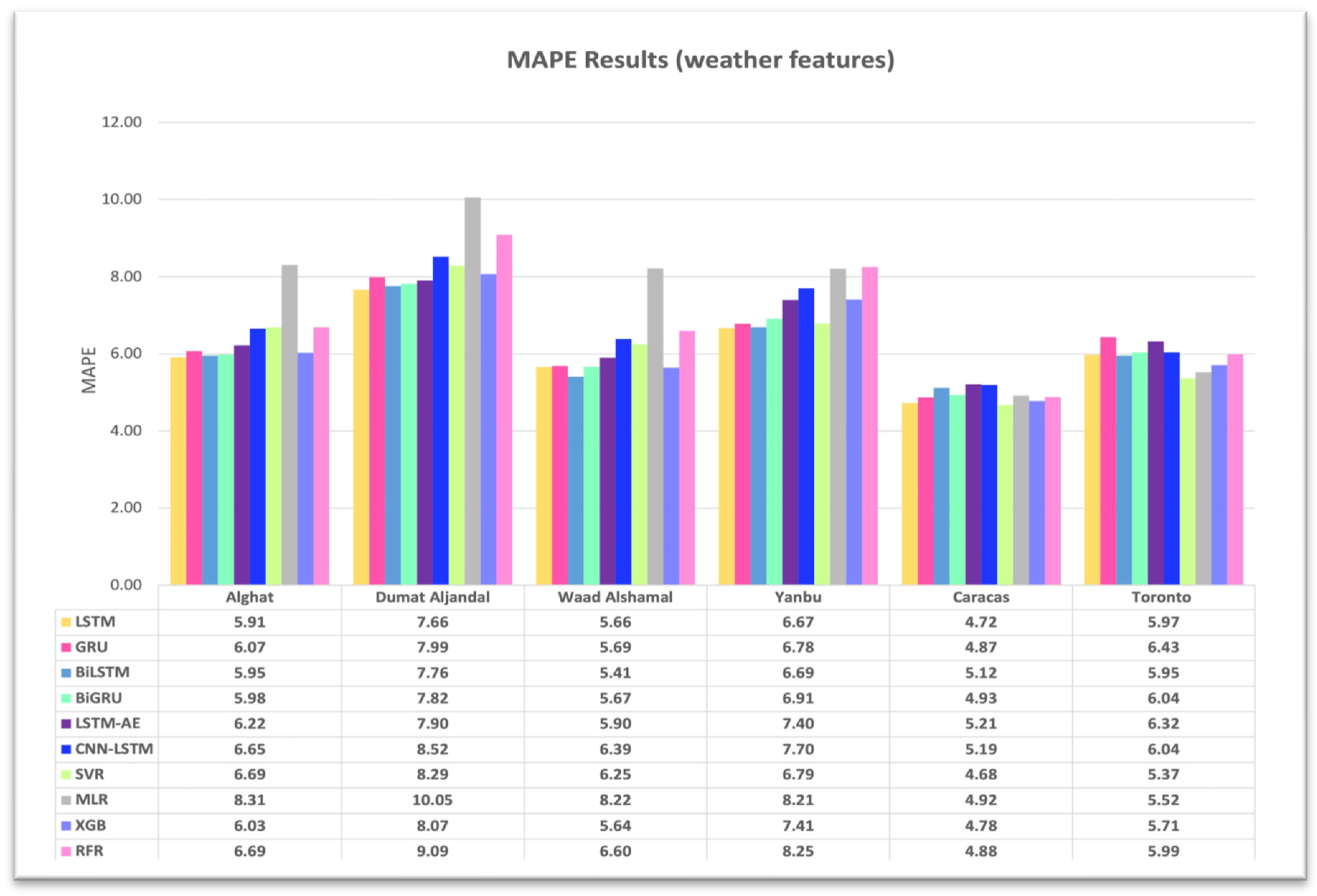
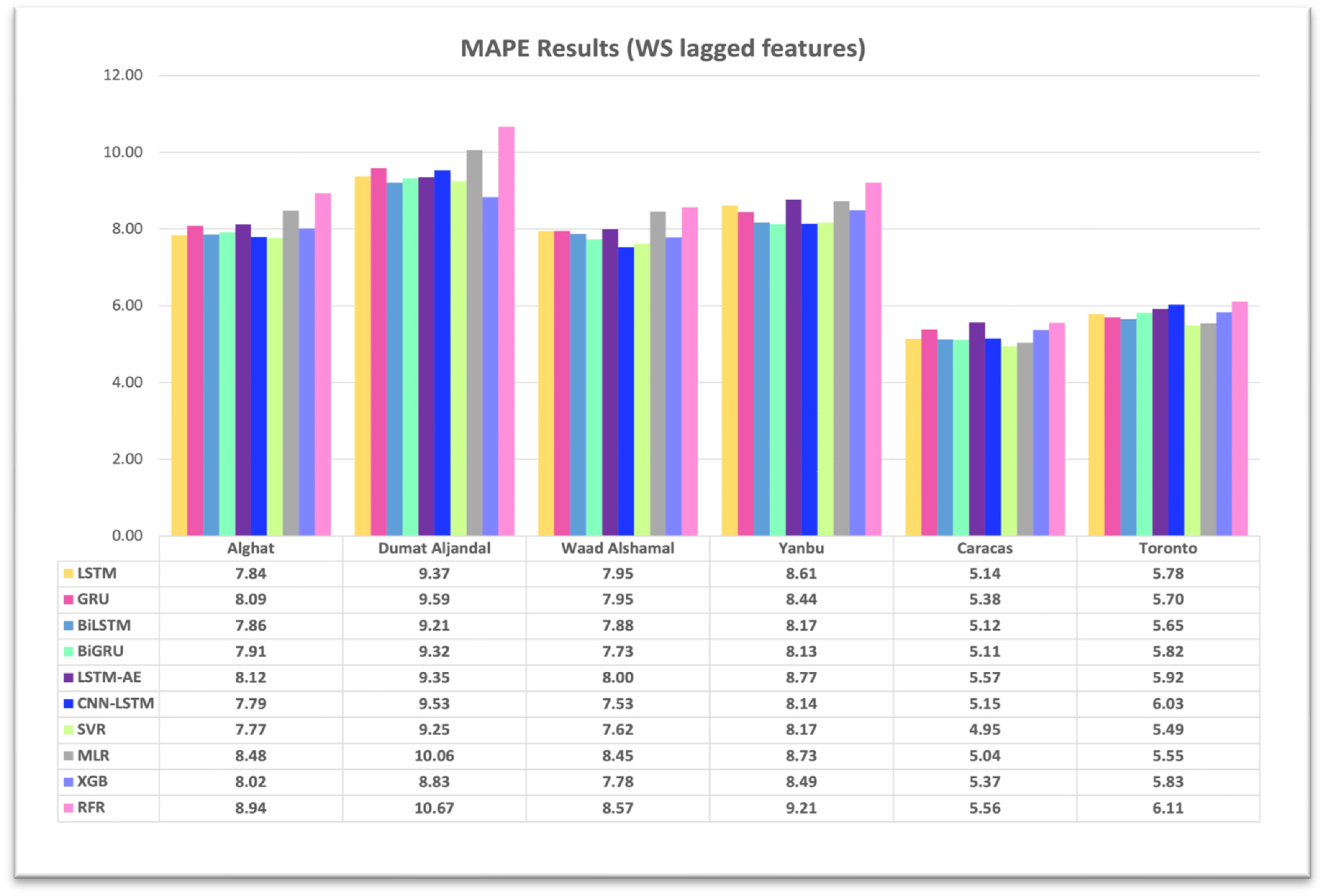
4.1. Effect of Using Last Hour’s Weather Variables on Forecasting
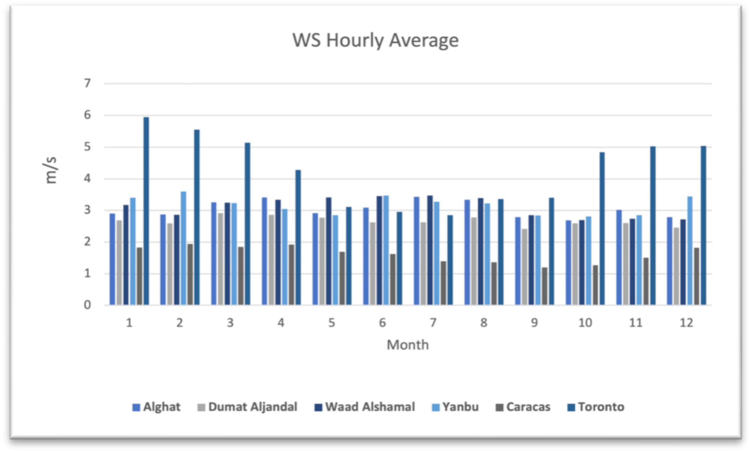
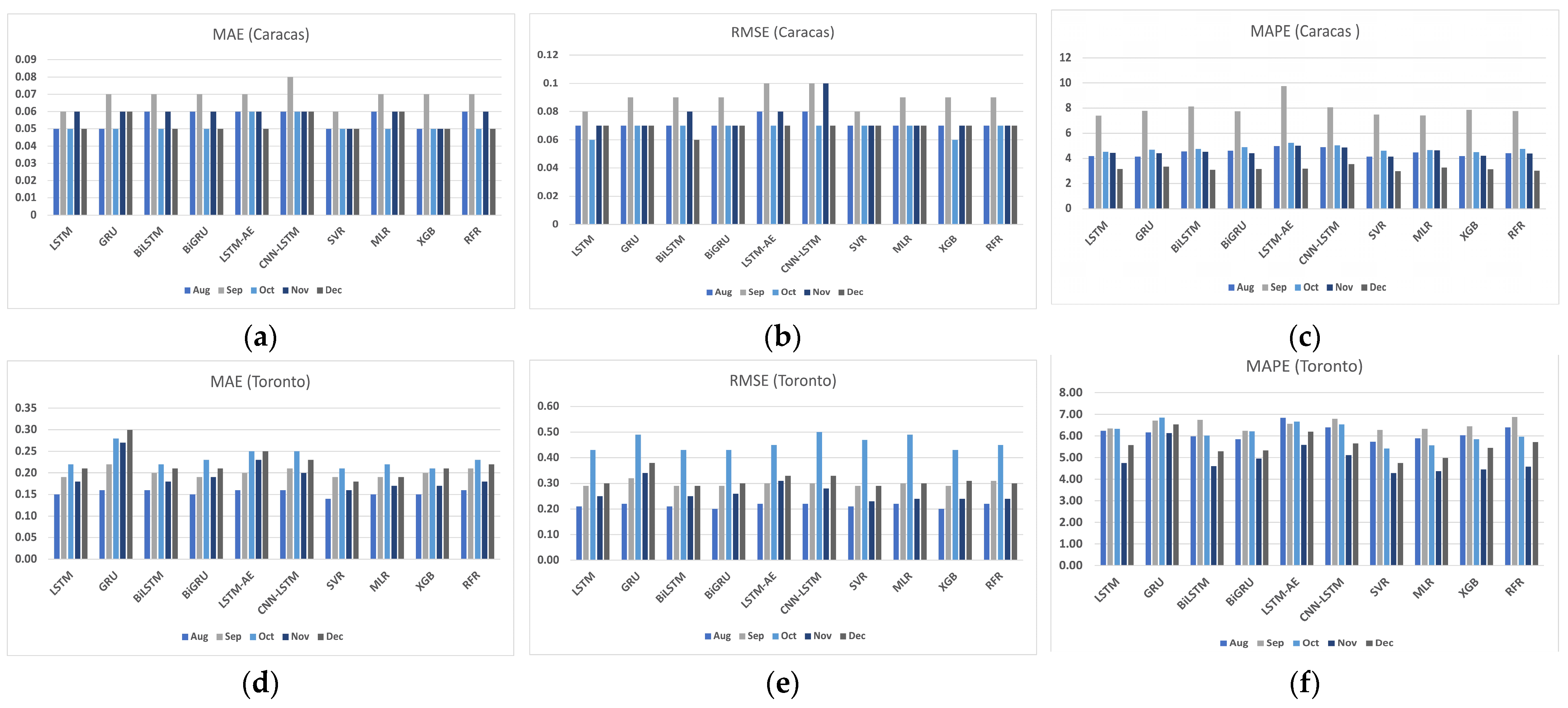
4.2. The Effect of Seasonality on Forecasting
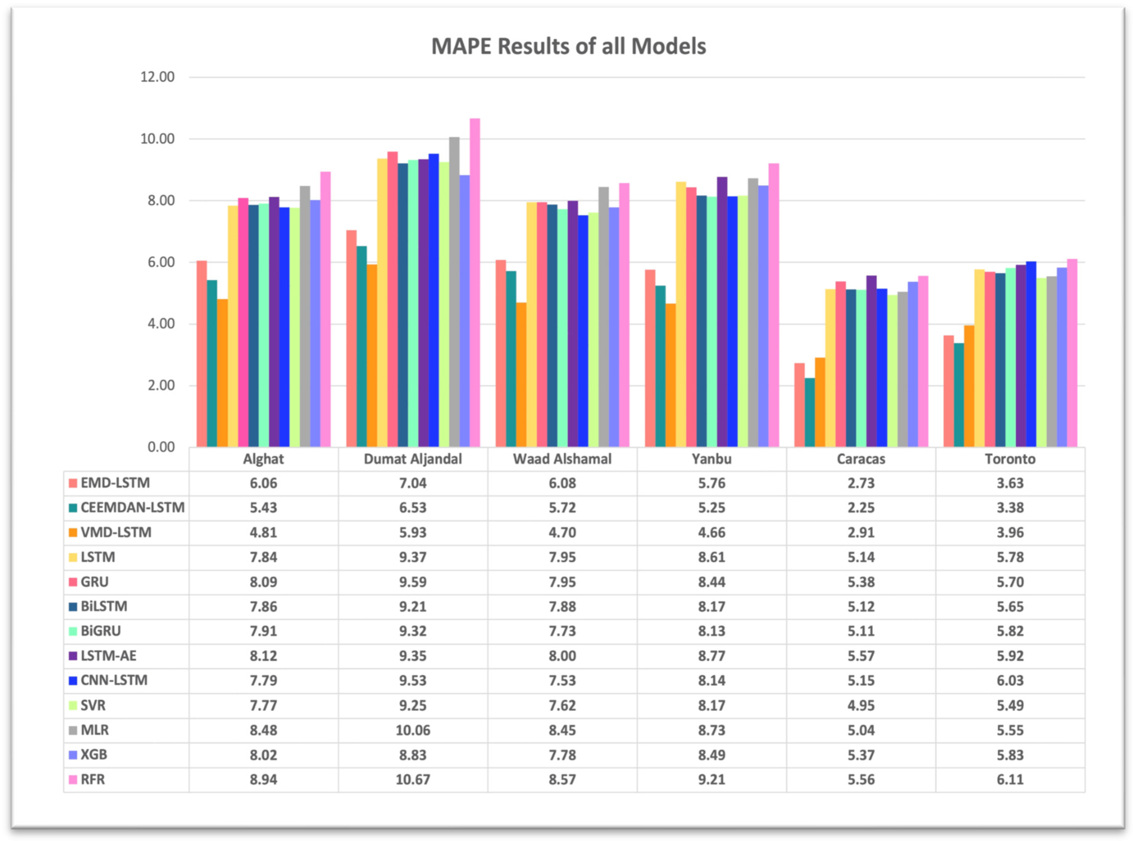
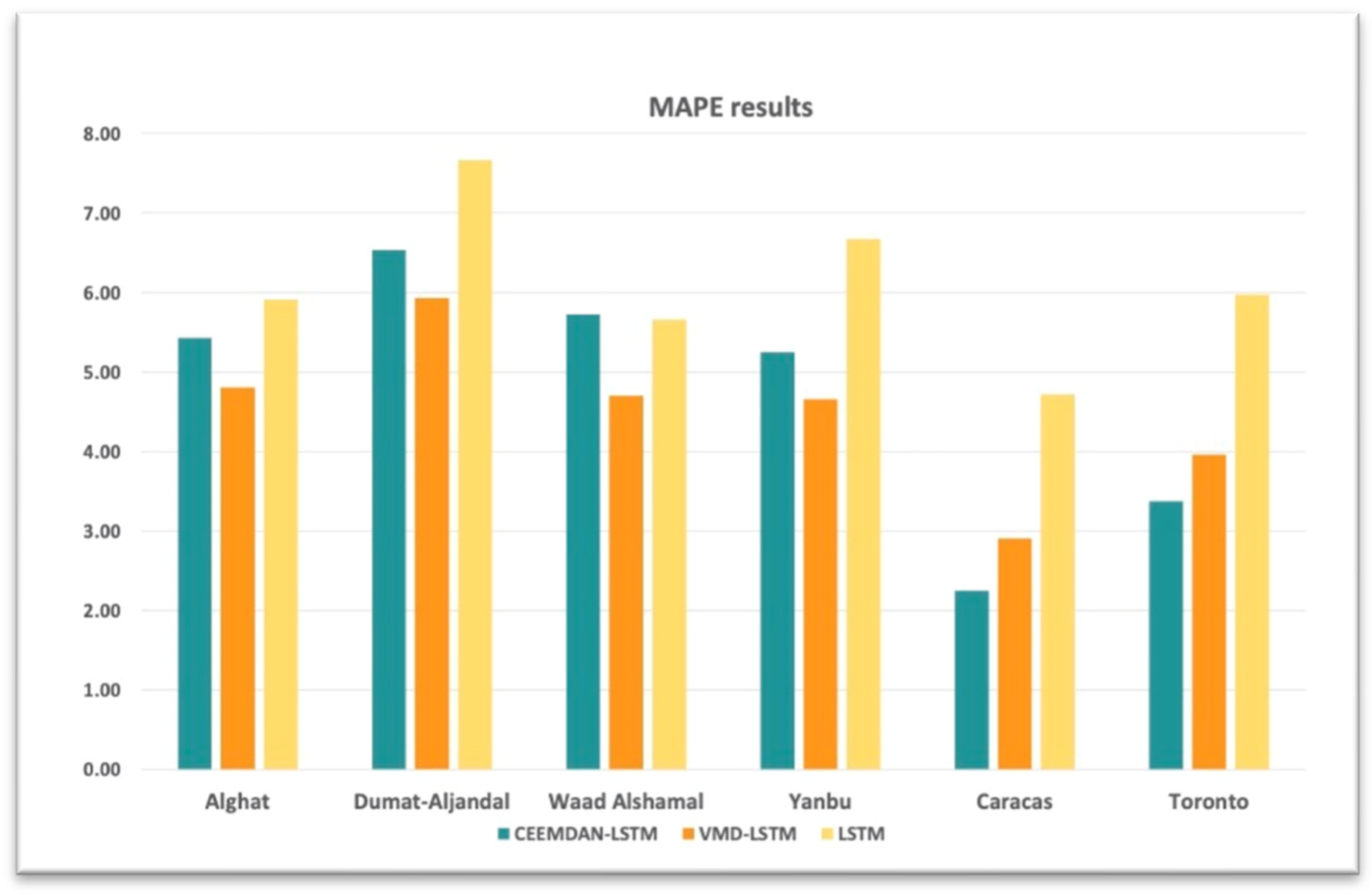
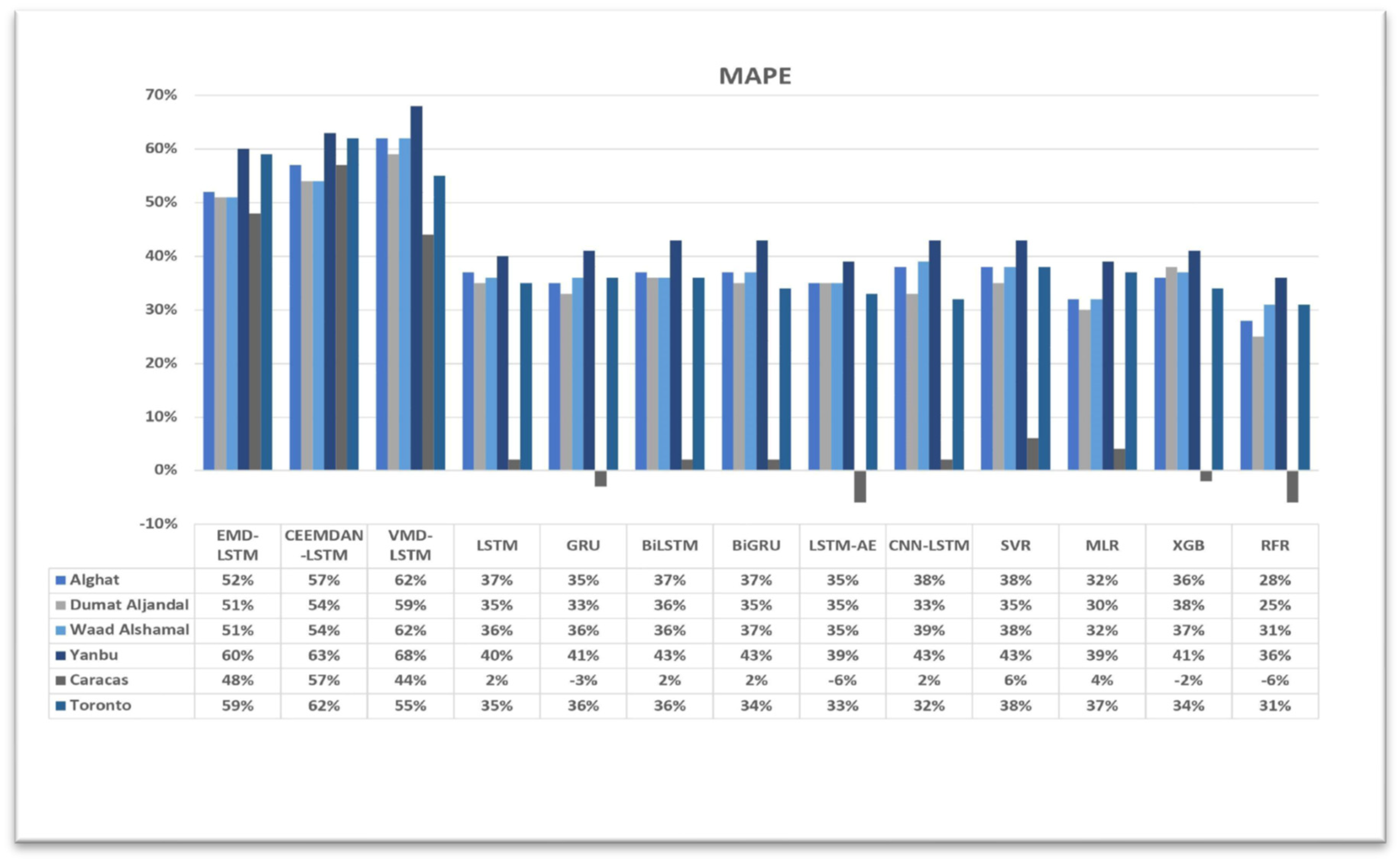
4.3. The Effect of Using Decomposition Methods on Forecasting
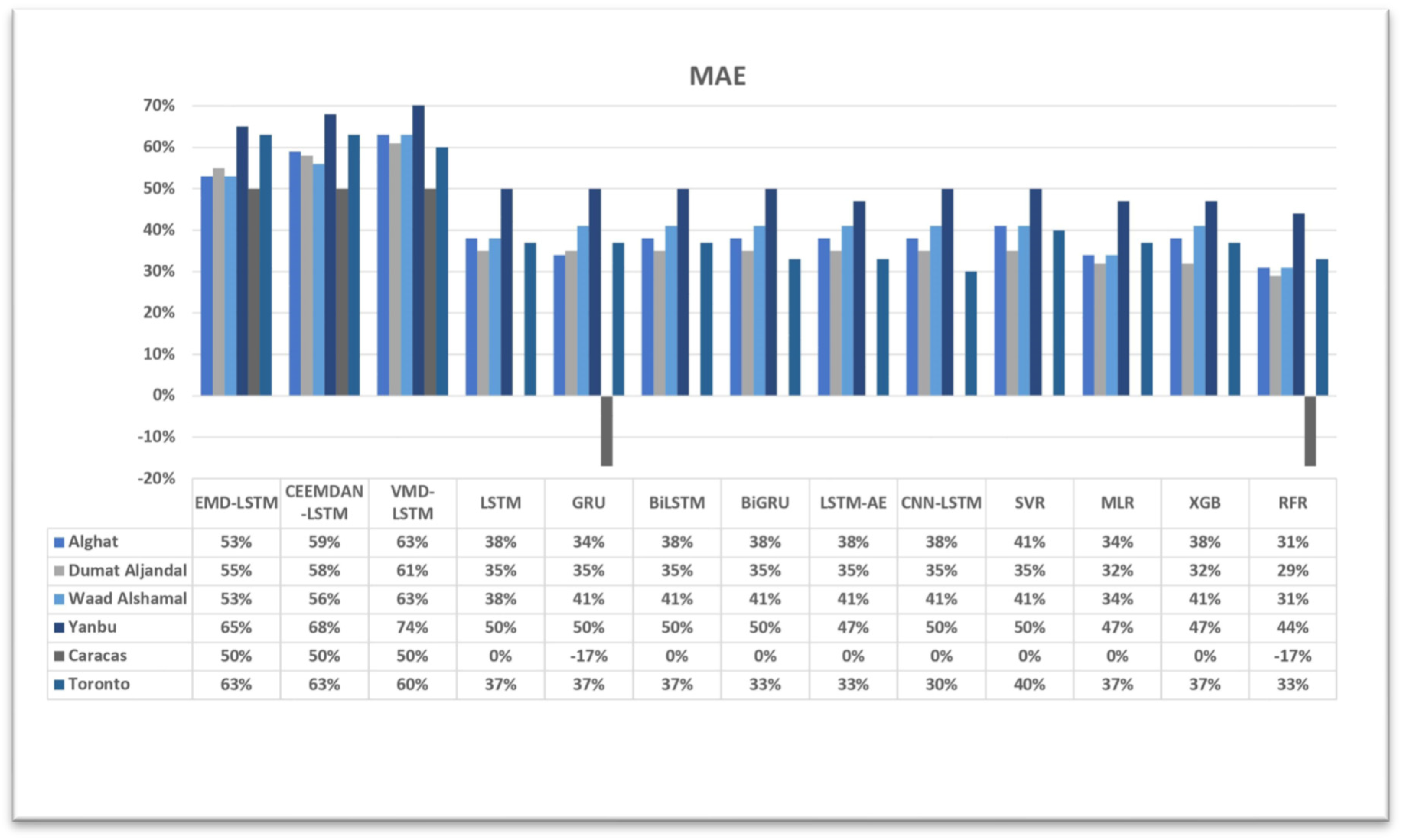
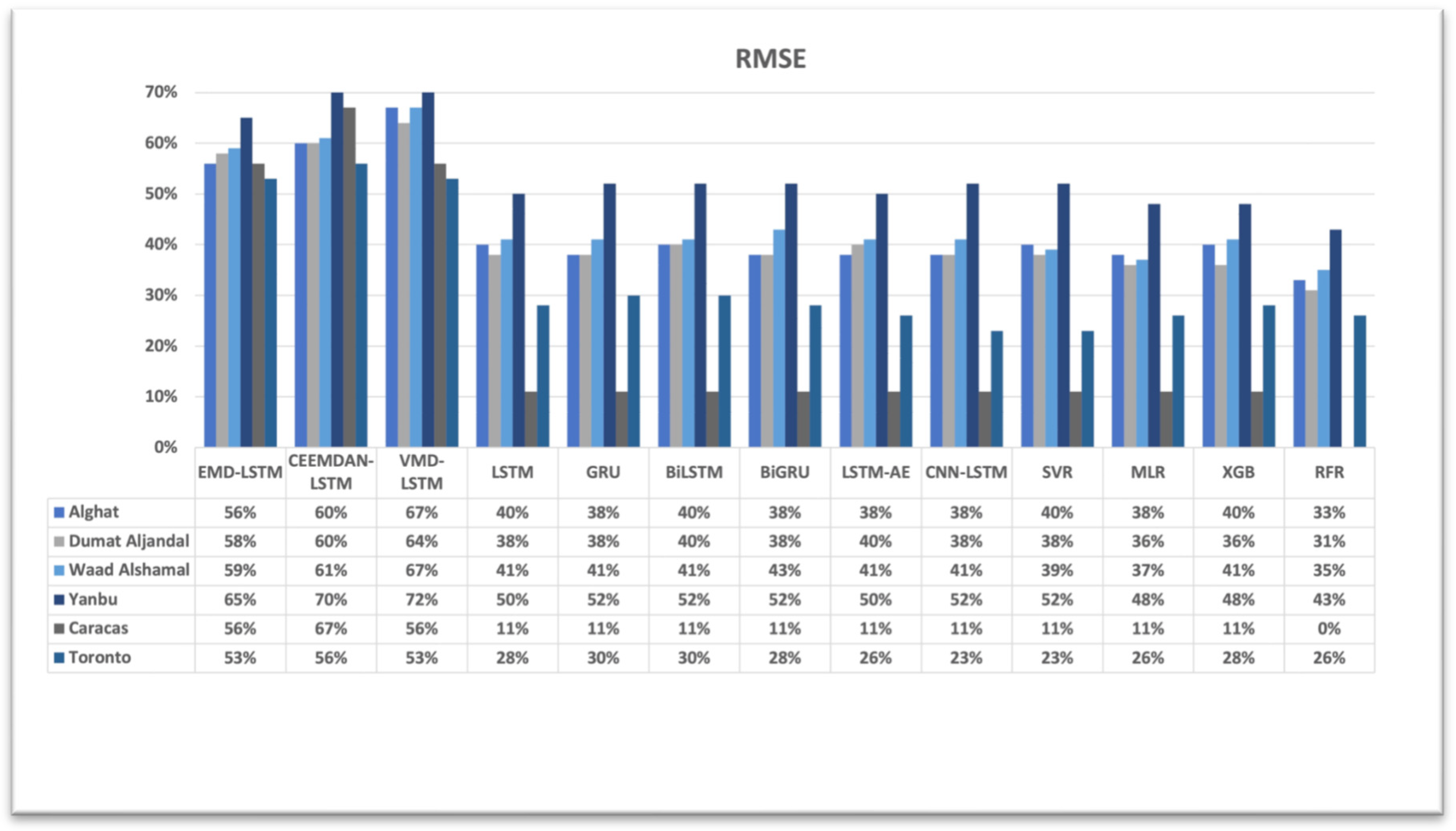
4.4. The FS of All Models
5. Conclusions
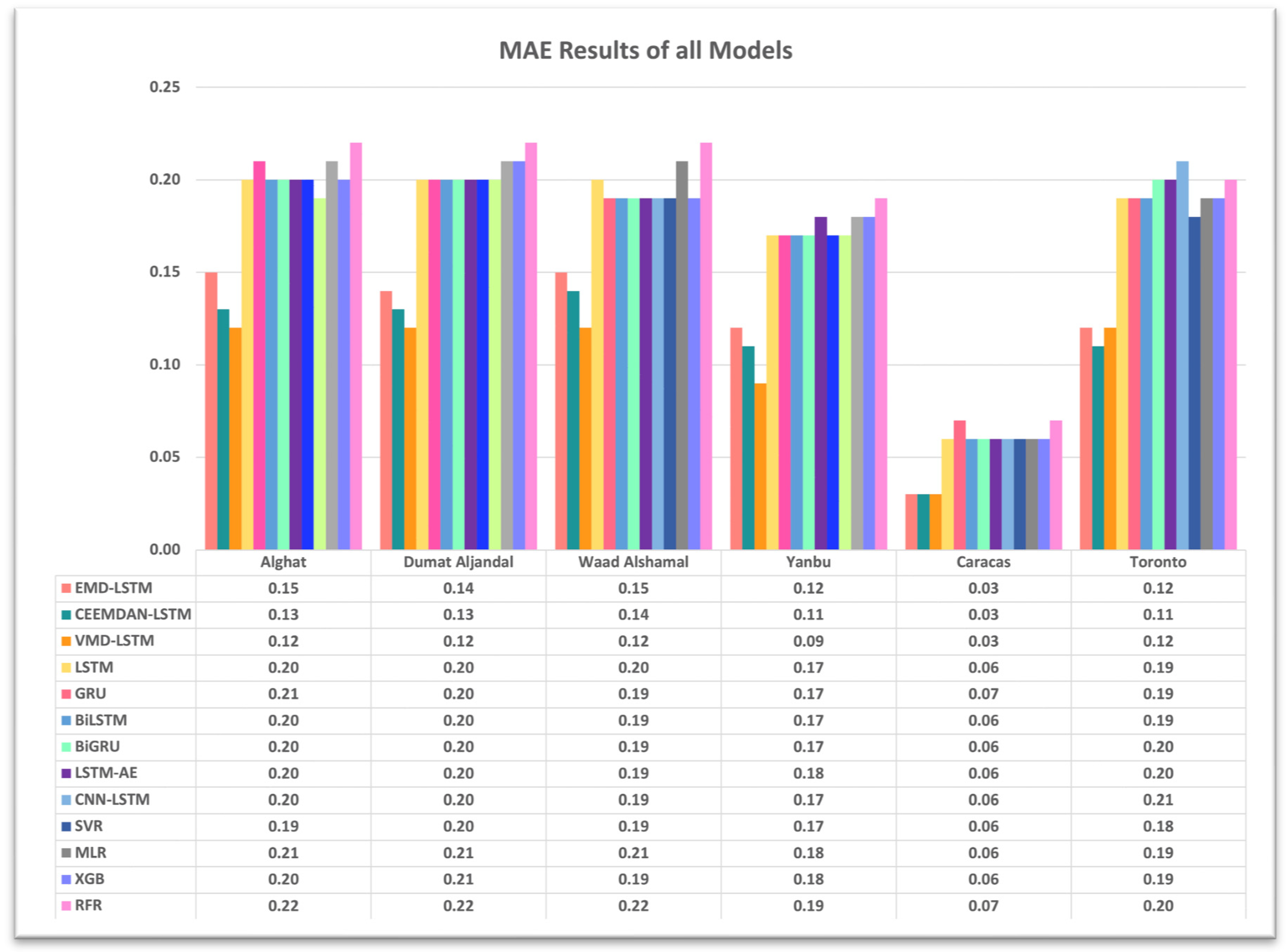
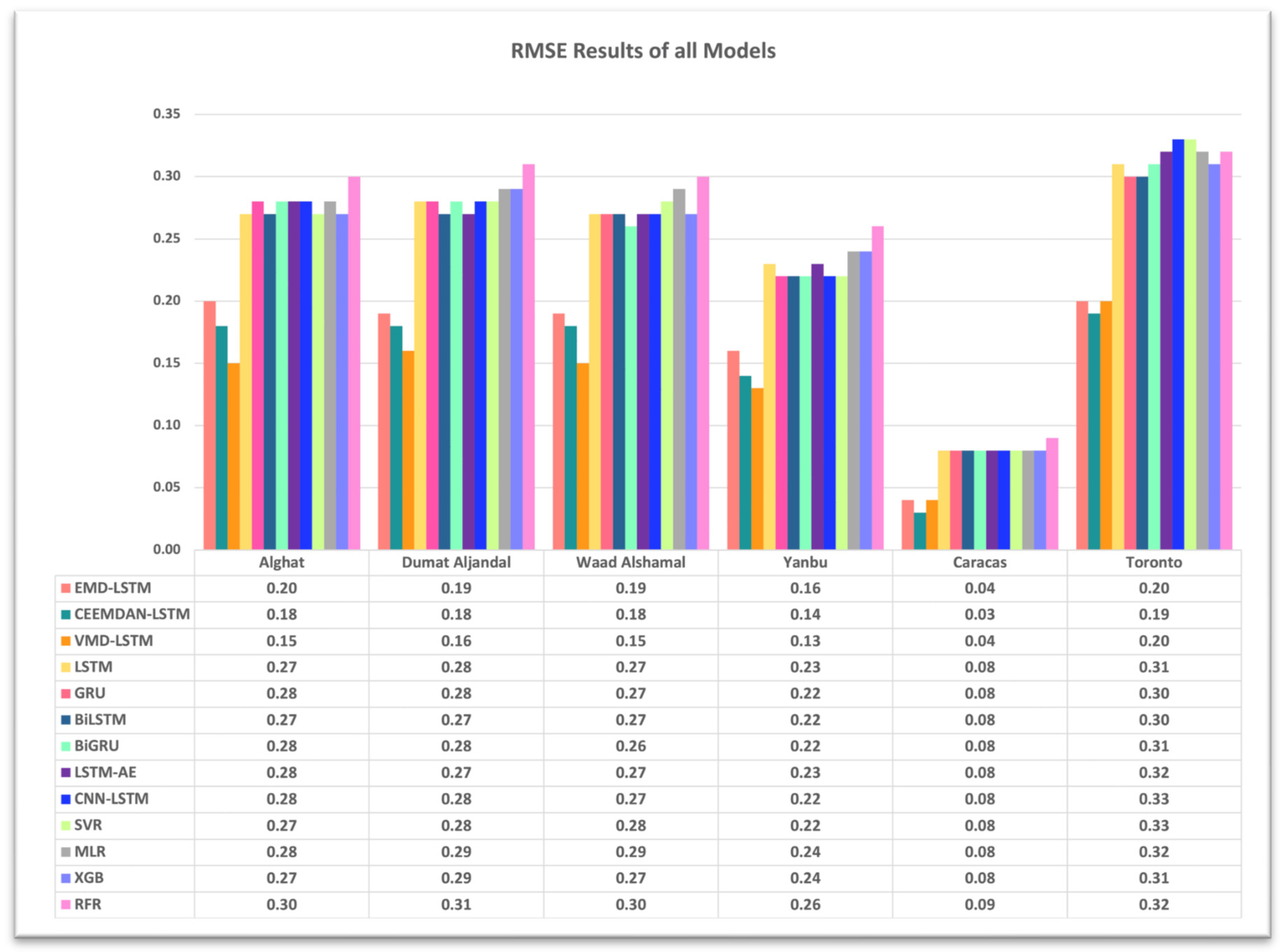
- The best forecasting model for the Saudi locations, according to MAE, RMSE, MAPE, and FS, is the hybrid model of VMD and the LSTM model.
- The best forecasting model for Caracas and Toronto, according to MAE, RMSE, MAPE, and FS, is the hybrid model of CEEMDAN and the LSTM model.
- All DL-based models have similar performance, but complex structures like the LSTM-AE and CNN-LSTM models have higher errors.
- Using the last hour’s weather variables, besides the last values of WS, improved the forecasting results for all models. However, the hybrid models with decomposition methods achieved better forecasting results.
- If seasons do not affect the hourly average of WS at the data source location, forecasting results would not show large variance either. Here, it is unnecessary to partition the datasets according to seasons and train separate forecasters.
Supplementary Materials
Author Contributions
Funding
Data Availability Statement
Conflicts of Interest
Abbreviations
| SA | Saudi Arabia |
| NWP | Numerical weather prediction |
| RNN | Recurrent neural network |
| AE | Autoencoder |
| LSTM | Long short-term memory |
| CNN | Convolutional neural network |
| GRU | Gated recurrent unit |
| BiLSTM | Bidirectional LSTM |
| BiGRU | Bidirectional GRU |
| RFR | Random forest regression |
| MLR | Multiple linear regression |
| MLP | Multilayer Perceptron Network |
| VMD | Variational mode decomposition |
| EMD | Empirical mode decomposition |
| CEEMDAN | Complete ensemble empirical mode decomposition with adaptive noise |
| SVR | Support vector regression |
| RMSE | Root mean square error |
| MAPE | Mean absolute percentage error |
| MAE | Mean absolute error |
| MSE | Mean squared error loss |
| WS | Wind speed |
| WD | Wind direction |
| WP | Wind power |
| T | Temperature |
| P | Pressure |
| RH | Relative humidity |
| ZA | Zenith Angle |
| PW | Precipitable Water |
| DP | Dew Point |
| HS | Hour sine |
| HC | Hour cosine |
| DS | Day sine |
| DC | Day cosine |
| WDS | Wind direction sine |
| WDC | Wind direction cosine |
| ML | Machine learning |
| DL | Deep learning |
| FFNN | Feed forward neural network |
| GHI | Global Horizontal Irradiation |
| DHI | Diffuse Horizontal Irradiation |
| DNI | Direct Normal Irradiance |
| WSTD | Wavelet soft threshold denoising |
| ReLU | Rectified Linear Unit |
| RR | Ridge regression |
| ESN | Echo state network |
| PE | Permutation entropy |
| RBFNN | Radial basis function neural network |
| IBA | Improved bat algorithm |
| FS | Forecast skill |
| XGB | eXtreme gradient boosting |
| ACF | Autocorrelation function |
| GA | Genetic algorithm |
| LN | Linear–nonlinear |
| MOBBSA | Multi-Objective Binary Back-tracking Search Algorithm |
| DE | Differential Evolution algorithm |
| NSRDB | National Solar Radiation Database |
| NREL | National Renewable Energy Laboratory |
| PSM | Physical Solar Model |
| SD | Standard deviation |
| VAR | Variance |
| IMF | Intrinsic mode function |
| MI | Mutual information |
References
- International Renewable Energy Agency (IRENA). Future of Wind—Executive Summary; IRENA: Masdar City, United Arab Emirates, 2019. [Google Scholar]
- Dumat Al Jandal Wind Farm in Saudi Arabia Starts Production. Available online: https://www.power-technology.com/news/dumat-al-jandal-wind/ (accessed on 24 February 2023).
- Giani, P.; Tagle, F.; Genton, M.G.; Castruccio, S.; Crippa, P. Closing the gap between wind energy targets and implementation for emerging countries. Appl. Energy 2020, 269, 115085. [Google Scholar] [CrossRef]
- Alharbi, F.; Csala, D. Saudi Arabia’s solar and wind energy penetration: Future performance and requirements. Energies 2020, 13, 588. [Google Scholar] [CrossRef]
- Zell, E.; Gasim, S.; Wilcox, S.; Katamoura, S.; Stoffel, T.; Shibli, H.; Engel-Cox, J.; Al Subie, M. Assessment of solar radiation resources in Saudi Arabia. Sol. Energy 2015, 119, 422–438. [Google Scholar] [CrossRef]
- Al Garni, H.Z.; Awasthi, A. Solar PV power plant site selection using a GIS-AHP based approach with application in Saudi Arabia. Appl. Energy 2017, 206, 1225–1240. [Google Scholar] [CrossRef]
- Saudi Press Agency. Saudi Arabia Announces Floating Five Projects to Produce Electricity with Use of Renewable Energy with Total Capacity of 3300 mw. 25 September 2022. Available online: https://www.spa.gov.sa/viewfullstory.php?lang=en&newsid=2386966 (accessed on 1 April 2023).
- Mohandes, M.A.; Rehman, S. Wind speed extrapolation using machine learning methods and LiDAR measurements. IEEE Access 2018, 6, 77634–77642. [Google Scholar] [CrossRef]
- Abualigah, L.; Zitar, R.A.; Almotairi, K.H.; Hussein, A.M.; Abd Elaziz, M.; Nikoo, M.R.; Gandomi, A.H. Wind, Solar, and Photovoltaic Renewable Energy Systems with and without Energy Storage Optimization: A Survey of Advanced Machine Learning and Deep Learning Techniques. Energies 2022, 15, 578. [Google Scholar] [CrossRef]
- Bali, V.; Kumar, A.; Gangwar, S. Deep learning based wind speed forecasting-A review. In Proceedings of the 2019 9th International Conference on Cloud Computing, Data Science & Engineering (Confluence), Noida, India, 10–11 January 2019; pp. 426–431. [Google Scholar]
- Deng, X.; Shao, H.; Hu, C.; Jiang, D.; Jiang, Y. Wind Power Forecasting Methods Based on Deep Learning: A Survey. Comput. Model. Eng. Sci. 2020, 122, 273–302. [Google Scholar] [CrossRef]
- Liu, H.; Chen, C.; Lv, X.; Wu, X.; Liu, M. Deterministic wind energy forecasting: A review of intelligent predictors and auxiliary methods. Energy Convers. Manag. 2019, 195, 328–345. [Google Scholar] [CrossRef]
- Alkhayat, G.; Mehmood, R. A Review and Taxonomy of Wind and Solar Energy Forecasting Methods Based on Deep Learning. Energy AI 2021, 4, 100060. [Google Scholar] [CrossRef]
- Mosavi, A.; Salimi, M.; Ardabili, S.F.; Rabczuk, T.; Shamshirband, S.; Varkonyi-Koczy, A.R. State of the art of machine learning models in energy systems, a systematic review. Energies 2019, 12, 1301. [Google Scholar] [CrossRef]
- Qian, Z.; Pei, Y.; Zareipour, H.; Chen, N. A review and discussion of decomposition-based hybrid models for wind energy forecasting applications. Appl. Energy 2019, 235, 939–953. [Google Scholar] [CrossRef]
- Zhao, L.; Li, Z.; Qu, L.; Zhang, J.; Teng, B. A hybrid VMD-LSTM/GRU model to predict non-stationary and irregular waves on the east coast of China. Ocean Eng. 2023, 276, 114136. [Google Scholar] [CrossRef]
- Sun, W.; Zhou, S.; Yang, J.; Gao, X.; Ji, J.; Dong, C. Artificial Intelligence Forecasting of Marine Heatwaves in the South China Sea Using a Combined U-Net and ConvLSTM System. Remote Sens. 2023, 15, 4068. [Google Scholar] [CrossRef]
- Bethel, B.J.; Sun, W.; Dong, C.; Wang, D. Forecasting hurricane-forced significant wave heights using a long short-term memory network in the Caribbean Sea. Ocean Sci. 2022, 18, 419–436. [Google Scholar] [CrossRef]
- Gao, Z.; Zhang, J. The fluctuation correlation between investor sentiment and stock index using VMD-LSTM: Evidence from China stock market. N. Am. J. Econ. Financ. 2023, 66, 101915. [Google Scholar] [CrossRef]
- Zhao, K.; Guo, D.; Sun, M.; Zhao, C.; Shuai, H. Short-Term Traffic Flow Prediction Based on VMD and IDBO-LSTM. IEEE Access 2023, 11, 97072–97088. [Google Scholar] [CrossRef]
- Sun, Z.; Zhao, M. Short-term wind power forecasting based on VMD decomposition, ConvLSTM networks and error analysis. IEEE Access 2020, 8, 134422–134434. [Google Scholar] [CrossRef]
- Lu, P.; Ye, L.; Pei, M.; Zhao, Y.; Dai, B.; Li, Z. Short-term wind power forecasting based on meteorological feature extraction and optimization strategy. Renew. Energy 2022, 184, 642–661. [Google Scholar] [CrossRef]
- Qin, G.; Yan, Q.; Zhu, J.; Xu, C.; Kammen, D.M. Day-ahead wind power forecasting based on wind load data using hybrid optimization algorithm. Sustainability 2021, 13, 1164. [Google Scholar] [CrossRef]
- Niu, D.; Sun, L.; Yu, M.; Wang, K. Point and interval forecasting of ultra-short-term wind power based on a data-driven method and hybrid deep learning model. Energy 2022, 254, 124384. [Google Scholar] [CrossRef]
- Yang, S.; Yang, H.; Li, N.; Ding, Z. Short-Term Prediction of 80–88 km Wind Speed in Near Space Based on VMD–PSO–LSTM. Atmosphere 2023, 14, 315. [Google Scholar] [CrossRef]
- Liu, B.; Xie, Y.; Wang, K.; Yu, L.; Zhou, Y.; Lv, X. Short-Term Multi-Step Wind Direction Prediction Based on OVMD Quadratic Decomposition and LSTM. Sustainability 2023, 15, 11746. [Google Scholar] [CrossRef]
- Duan, J.; Wang, P.; Ma, W.; Tian, X.; Fang, S.; Cheng, Y.; Chang, Y.; Liu, H. Short-term wind power forecasting using the hybrid model of improved variational mode decomposition and Correntropy Long Short-term memory neural network. Energy 2021, 214, 118980. [Google Scholar] [CrossRef]
- Xu, W.; Liu, P.; Cheng, L.; Zhou, Y.; Xia, Q.; Gong, Y.; Liu, Y. Multi-step wind speed prediction by combining a WRF simulation and an error correction strategy. Renew. Energy 2021, 163, 772–782. [Google Scholar] [CrossRef]
- Qian, J.; Zhu, M.; Zhao, Y.; He, X. Short-term wind speed prediction with a two-layer attention-based LSTM. Comput. Syst. Sci. Eng. 2021, 39, 197–209. [Google Scholar] [CrossRef]
- Li, Y.; Chen, X.; Li, C.; Tang, G.; Gan, Z.; An, X. A hybrid deep interval prediction model for wind speed forecasting. IEEE Access 2020, 9, 7323–7335. [Google Scholar] [CrossRef]
- Zhang, M.; Ni, Q.; Zhao, S.; Wang, Y.; Shen, C. A combined prediction method for short-term wind speed using variational mode decomposition based on parameter optimization. In Proceedings of the 2020 IEEE International Conference on Systems, Man, and Cybernetics (SMC), Toronto, ON, Canada, 11–14 October 2020; pp. 2607–2614. [Google Scholar]
- Liao, X.; Liu, Z.; Deng, W. Short-term wind speed multistep combined forecasting model based on two-stage decomposition and LSTM. Wind Energy 2021, 24, 991–1012. [Google Scholar] [CrossRef]
- Ma, Z.; Chen, H.; Wang, J.; Yang, X.; Yan, R.; Jia, J.; Xu, W. Application of hybrid model based on double decomposition, error correction and deep learning in short-term wind speed prediction. Energy Convers. Manag. 2020, 205, 112345. [Google Scholar] [CrossRef]
- Zeng, L.; Lan, X.; Wang, S. Short-term wind power prediction based on the combination of numerical weather forecast and time series. J. Renew. Sustain. Energy 2023, 15, 013303. [Google Scholar] [CrossRef]
- Han, L.; Zhang, R.; Wang, X.; Bao, A.; Jing, H. Multi-step wind power forecast based on VMD-LSTM. IET Renew. Power Gener. 2019, 13, 1690–1700. [Google Scholar] [CrossRef]
- Xing, F.; Song, X.; Wang, Y.; Qin, C. A New Combined Prediction Model for Ultra-Short-Term Wind Power Based on Variational Mode Decomposition and Gradient Boosting Regression Tree. Sustainability 2023, 15, 11026. [Google Scholar] [CrossRef]
- Han, L.; Jing, H.; Zhang, R.; Gao, Z. Wind power forecast based on improved Long Short Term Memory network. Energy 2019, 189, 116300. [Google Scholar] [CrossRef]
- Yin, H.; Ou, Z.; Huang, S.; Meng, A. A cascaded deep learning wind power prediction approach based on a two-layer of mode decomposition. Energy 2019, 189, 116316. [Google Scholar] [CrossRef]
- Ai, X.; Li, S.; Xu, H. Short-term wind speed forecasting based on two-stage preprocessing method, sparrow search algorithm and long short-term memory neural network. Energy Rep. 2022, 8, 14997–15010. [Google Scholar] [CrossRef]
- Goh, H.H.; He, R.; Zhang, D.; Liu, H.; Dai, W.; Lim, C.S.; Kurniawan, T.A.; Teo, K.T.; Goh, K.C. Short-term wind power prediction based on preprocessing and improved secondary decomposition. J. Renew. Sustain. Energy 2021, 13, 053302. [Google Scholar] [CrossRef]
- Liu, Z.; Liu, H. A novel hybrid model based on GA-VMD, sample entropy reconstruction and BiLSTM for wind speed prediction. Measurement 2023, 222, 113643. [Google Scholar] [CrossRef]
- Wang, S.; Liu, C.; Liang, K.; Cheng, Z.; Kong, X.; Gao, S. Wind speed prediction model based on improved VMD and sudden change of wind speed. Sustainability 2022, 14, 8705. [Google Scholar] [CrossRef]
- Tang, J.; Chien, Y.-R. Research on Wind Power Short-Term Forecasting Method Based on Temporal Convolutional Neural Network and Variational Modal Decomposition. Sensors 2022, 22, 7414. [Google Scholar] [CrossRef]
- Sibtain, M.; Bashir, H.; Nawaz, M.; Hameed, S.; Azam, M.I.; Li, X.; Abbas, T.; Saleem, S. A multivariate ultra-short-term wind speed forecasting model by employing multistage signal decomposition approaches and a deep learning network. Energy Convers. Manag. 2022, 263, 115703. [Google Scholar] [CrossRef]
- Liang, T.; Xie, G.; Fan, S.; Meng, Z. A Combined Model Based on CEEMDAN, Permutation Entropy, Gated Recurrent Unit Network, and an Improved Bat Algorithm for Wind Speed Forecasting. IEEE Access 2020, 8, 165612–165630. [Google Scholar] [CrossRef]
- Lv, S.-X.; Wang, L. Deep learning combined wind speed forecasting with hybrid time series decomposition and multi-objective parameter optimization. Appl. Energy 2022, 311, 118674. [Google Scholar] [CrossRef]
- Yildiz, C.; Acikgoz, H.; Korkmaz, D.; Budak, U. An improved residual-based convolutional neural network for very short-term wind power forecasting. Energy Convers. Manag. 2021, 228, 113731. [Google Scholar] [CrossRef]
- Hu, H.; Wang, L.; Tao, R. Wind speed forecasting based on variational mode decomposition and improved echo state network. Renew. Energy 2021, 164, 729–751. [Google Scholar] [CrossRef]
- Manero, J.; Béjar, J.; Cortés, U. ‘Dust in the wind…’, deep learning application to wind energy time series forecasting. Energies 2019, 12, 2385. [Google Scholar] [CrossRef]
- Peng, Z.; Peng, S.; Fu, L.; Lu, B.; Tang, J.; Wang, K.; Li, W. A novel deep learning ensemble model with data denoising for short-term wind speed forecasting. Energy Convers. Manag. 2020, 207, 112524. [Google Scholar] [CrossRef]
- Alhussein, M.; Haider, S.I.; Aurangzeb, K. Microgrid-level energy management approach based on short-term forecasting of wind speed and solar irradiance. Energies 2019, 12, 1487. [Google Scholar] [CrossRef]
- Lawal, A.; Rehman, S.; Alhems, L.M.; Alam, M.M. Wind speed prediction using hybrid 1D CNN and BLSTM network. IEEE Access 2021, 9, 156672–156679. [Google Scholar] [CrossRef]
- Huang, H.; Castruccio, S.; Genton, M.G. Forecasting high-frequency spatio-temporal wind power with dimensionally reduced echo state networks. arXiv 2021, arXiv:2102.01141. [Google Scholar] [CrossRef]
- Alharbi, F.R.; Csala, D. Wind speed and solar irradiance prediction using a bidirectional long short-term memory model based on neural networks. Energies 2021, 14, 6501. [Google Scholar] [CrossRef]
- Alharbi, F.R.; Csala, D. Short-Term Wind Speed and Temperature Forecasting Model Based on Gated Recurrent Unit Neural Networks. In Proceedings of the 2021 3rd Global Power, Energy and Communication Conference (GPECOM), Antalya, Turkey, 5–8 October 2021; pp. 142–147. [Google Scholar]
- Brahimi, T. Using Artificial Intelligence to Predict Wind Speed for Energy Application in Saudi Arabia. Energies 2019, 12, 4669. [Google Scholar] [CrossRef]
- Faniband, Y.P.; Shaahid, S.M. Forecasting Wind Speed using Artificial Neural Networks–A Case Study of a Potential Location of Saudi Arabia. in E3S Web Conf. 2020, 173, 1004. [Google Scholar] [CrossRef]
- Faniband, Y.P.; Shaahid, S.M. Univariate Time Series Prediction of Wind speed with a case study of Yanbu, Saudi Arabia. Int. J. 2021, 10, 257–264. [Google Scholar]
- Zheng, Y.; Ge, Y.; Muhsen, S.; Wang, S.; Elkamchouchi, D.H.; Ali, E.; Ali, H.E. New ridge regression, artificial neural networks and support vector machine for wind speed prediction. Adv. Eng. Softw. 2023, 179, 103426. [Google Scholar] [CrossRef]
- Salman, U.T.; Rehman, S.; Alawode, B.; Alhems, L.M. Short term prediction of wind speed based on long-short term memory networks. FME Trans. 2021, 49, 643–652. [Google Scholar] [CrossRef]
- mindat.org. Available online: https://www.mindat.org/climate.php (accessed on 25 October 2023).
- Sengupta, M.; Habte, A.; Xie, Y.; Lopez, A.; Buster, G. National Solar Radiation Database (NSRDB). United States. 2018. Available online: https://data.openei.org/submissions/1 (accessed on 15 January 2022). [CrossRef]
- Petneházi, G. Recurrent neural networks for time series forecasting. arXiv 2019, arXiv:1901.00069. [Google Scholar]
- Chen, J.; Zhu, Q.; Li, H.; Zhu, L.; Shi, D.; Li, Y.; Duan, X.; Liu, Y. Learning Heterogeneous Features Jointly: A Deep End-to-End Framework for Multi-Step Short-Term Wind Power Prediction. IEEE Trans. Sustain. Energy 2020, 11, 1761–1772. [Google Scholar] [CrossRef]
- Memarzadeh, G.; Keynia, F. A new short-term wind speed forecasting method based on fine-tuned LSTM neural network and optimal input sets. Energy Convers. Manag. 2020, 213, 112824. [Google Scholar] [CrossRef]
- Gholamy, A.; Kreinovich, V.; Kosheleva, O. Why 70/30 or 80/20 Relation between Training and Testing Sets: A Pedagogical Explanation. 2018. Available online: https://scholarworks.utep.edu/cs_techrep/1209/ (accessed on 23 October 2023).
- Liu, H.; Chen, C. Data processing strategies in wind energy forecasting models and applications: A comprehensive review. Appl. Energy 2019, 249, 392–408. [Google Scholar] [CrossRef]
- Peng, T.; Zhang, C.; Zhou, J.; Nazir, M.S. An integrated framework of Bi-directional Long-Short Term Memory (BiLSTM) based on sine cosine algorithm for hourly solar radiation forecasting. Energy 2021, 221, 119887. [Google Scholar] [CrossRef]
- Zhou, H.; Zhang, Y.; Yang, L.; Liu, Q.; Yan, K.; Du, Y. Short-term photovoltaic power forecasting based on long short term memory neural network and attention mechanism. IEEE Access 2019, 7, 78063–78074. [Google Scholar] [CrossRef]
- Sorkun, M.C.; Paoli, C.; Incel, Ö.D. Time series forecasting on solar irradiation using deep learning. In Proceedings of the 2017 10th International Conference on Electrical and Electronics Engineering (ELECO), Bursa, Turkey, 30 November 2017–2 December 2017; pp. 151–155. [Google Scholar]
- Lynn, H.M.; Pan, S.B.; Kim, P. A deep bidirectional GRU network model for biometric electrocardiogram classification based on recurrent neural networks. IEEE Access 2019, 7, 145395–145405. [Google Scholar] [CrossRef]
- Nguyen, H.D.; Tran, K.P.; Thomassey, S.; Hamad, M. Forecasting and Anomaly Detection approaches using LSTM and LSTM Autoencoder techniques with the applications in supply chain management. Int. J. Inf. Manag. 2021, 57, 102282. [Google Scholar] [CrossRef]
- Sagheer, A.; Kotb, M. Unsupervised pre-training of a deep LSTM-based stacked autoencoder for multivariate time series forecasting problems. Sci. Rep. 2019, 9, 19038. [Google Scholar] [CrossRef]
- Nguyen, T.H.T.; Phan, Q.B. Hourly day ahead wind speed forecasting based on a hybrid model of EEMD, CNN-Bi-LSTM embedded with GA optimization. Energy Rep. 2022, 8, 53–60. [Google Scholar] [CrossRef]
- Drisya, G.V.; Asokan, K.; Kumar, K.S. Wind speed forecast using random forest learning method. arXiv 2022, arXiv:2203.14909. [Google Scholar]
- Jiang, Z.; Che, J.; He, M.; Yuan, F. A CGRU multi-step wind speed forecasting model based on multi-label specific XGBoost feature selection and secondary decomposition. Renew. Energy 2023, 203, 802–827. [Google Scholar] [CrossRef]
- Barhmi, S.; Elfatni, O.; Belhaj, I. Forecasting of wind speed using multiple linear regression and artificial neural networks. Energy Syst. 2020, 11, 935–946. [Google Scholar] [CrossRef]
- Li, G.; Xie, S.; Wang, B.; Xin, J.; Li, Y.; Du, S. Photovoltaic Power Forecasting With a Hybrid Deep Learning Approach. IEEE Access 2020, 8, 175871–175880. [Google Scholar] [CrossRef]
- Hossain, M.S.; Mahmood, H. Short-term photovoltaic power forecasting using an LSTM neural network and synthetic weather forecast. IEEE Access 2020, 8, 172524–172533. [Google Scholar] [CrossRef]
- Voyant, C.; Notton, G.; Kalogirou, S.; Nivet, M.L.; Paoli, C.; Motte, F.; Fouilloy, A. Machine learning methods for solar radiation forecasting: A review. Renew. Energy 2017, 105, 569–582. [Google Scholar] [CrossRef]
- Ramli, M.A.M.; Twaha, S.; Al-Hamouz, Z. Analyzing the potential and progress of distributed generation applications in Saudi Arabia: The case of solar and wind resources. Renew. Sustain. Energy Rev. 2017, 70, 287–297. [Google Scholar] [CrossRef]
- Yan, X.; Liu, Y.; Xu, Y.; Jia, M. Multistep forecasting for diurnal wind speed based on hybrid deep learning model with improved singular spectrum decomposition. Energy Convers. Manag. 2020, 225, 113456. [Google Scholar] [CrossRef]
- Wang, D.; Luo, H.; Grunder, O.; Lin, Y. Multi-step ahead wind speed forecasting using an improved wavelet neural network combining variational mode decomposition and phase space reconstruction. Renew. Energy 2017, 113, 1345–1358. [Google Scholar] [CrossRef]
- Liu, H.; Mi, X.; Li, Y. Smart multi-step deep learning model for wind speed forecasting based on variational mode decomposition, singular spectrum analysis, LSTM network and ELM. Energy Convers. Manag. 2018, 159, 54–64. [Google Scholar] [CrossRef]
- Wang, X.; Yu, Q.; Yang, Y. Short-term wind speed forecasting using variational mode decomposition and support vector regression. J. Intell. Fuzzy Syst. 2018, 34, 3811–3820. [Google Scholar] [CrossRef]
- Alkhayat, G.; Hasan, S.H.; Mehmood, R. SENERGY: A Novel Deep Learning-Based Auto-Selective Approach and Tool for Solar Energy Forecasting. Energies 2022, 15, 6659. [Google Scholar] [CrossRef]


| Ref No. | Aim | Method | Features | Data | Climate | Results | Location | Limitation |
|---|---|---|---|---|---|---|---|---|
| [22] | WP | Hybrid of VMD + WPE + CNN LSTM | WP, WS, WD, Momentum flux | G | Dwa/Dwb, BSk | NRMSE = 4.19%, NMAE = 3.72%. | Four wind farms, China | A |
| NRMSE = 4.96%, NMAE = 3.51%. | ||||||||
| NRMSE = 5.03%, NMAE = 4.89%. | ||||||||
| NRMSE = 5.13%, NMAE = 4.75. | ||||||||
| [33] | WS | Hybrid of CEEMDAN + VMD + LSTM | WS | G | Dfb | RMSE = 0.23, MAE = 0.17, MAPE = 4.45% for series 3. RMSE = 0.29, MAE = 0.19, MAPE = 5.38% for series 4. | Colorado, USA | A |
| [45] | WS | Hybrid of CEEMDAN + PE + GRU + RBFNN + IBA | WS | G | BSk | MAE = 0.45, RMSE = 0.59, MAPE = 4.79%. | Zhangjiakou, China | A |
| [46] | WS | Hybrid of VMD + LN + MOBBSA + LSTM-AE | WS | G | Dfc | MAE = 0.08, RMSE = 0.11, MAPE = 2.95%. | Rocky Mountains, USA | A |
| [47] | WP | Hybrid of VMD+ CNN | WP, WS, WD | G | Cfa | R = 0.97, RMSE = 0.05, MAE = 0.04. | A location in Turkey | A |
| [48] | WS | Hybrid of VMD +ESN+ DE | WS, WD, T, P, RH, | G | Csb | RMSE = 0.12, MAE = 0.10, MAPE = 2.6%. | Galicia, Spain | A |
| [49] | WS | MLP, CNN, RNN | WS | S | Multiple | R2 for CNN and RNN model is higher than MLP. | Locations in USA | A, B |
| [50] | WS | Hybrid of WSTD + GRU | WS | G | Dwa, Cfa, BSk | RMSE = 0.38, MAPE = 0.01. | Bondvill, USA | A |
| RMSE = 0.26, MAPE = 0.07. | Penn State, USA | |||||||
| RMSE = 0.53, MAPE = 0.03. | Boulder, USA | |||||||
| RMSE = 1.86, MAPE = 0.19. | Desert Rock, USA | |||||||
| [51] | WS | CNN | T, RH, P, WS, season, M, D, H | S | Csc | MAE = 0.09, RMSE = 0.13, sMAPE = 4.92. | San Francisco, USA | A, B |
| [52] | WS | CNN-BiLSTM | WS, SD, MAX | G | BWh | MAE = 0.30, RMSE = 0.43, MAPE = 115 | Location in SA | B |
| [53] | WS | ESN | WS | S | BWh | MSE = 0.24. | Location in SA | B |
| [54] | WS | BiLSTM | WS, GHI, DNI, DHI, T | S | BWh | MAE = 0.4, RMSE = 0.6, MAPE = 15. | Dumat Al Jandal, SA | B |
| [55] | WS | GRU | WS, T | S | BWh | MAE = 0.48, RMSE = 0.66, MAPE = 5. | B | |
| [56] | WS | FFNN | T, WD, P, GHI, RH, PWS | G | BWh | RMSE = 0.81, R2 = 0.92, MAE = 0.61. | Jeddah, SA | B |
| RMSE = 1.12, R2 = 0.90. | Afif, SA | |||||||
| RMSE = 0.54, R2 = 0.87. | Riyadh, SA | |||||||
| RMSE = 0.86, R2 = 0.90. | Taif, SA | |||||||
| [57] | WS | FFNN | WS, T, RH | G | BWh | MAPE = 6.65%, MSE = 0.09. | Qaisumah, SA | B |
| [58] | WS | SVR | WS | G | BWh | MAE = 2.37, MAPE = 206.80. | Yanbu, SA | B |
| [59] | WS | RR | WS, WD, PWS, T, P, RH | S | BWh | MAE = 1.22, RMSE = 0.26, R2 = 0.9. | A city in SA | B |
| [60] | WS | LSTM | WS, T, P | G | BWh | MAE = 0.28, R2 = 0.97. | Dhahran, SA | B |
| Location No. | Location Name | Latitude (N) | Longitude (E) | Elevation (m) |
|---|---|---|---|---|
| 1 | Alghat | 26.32 | 43.45 | 674 |
| 2 | Dumat Al Jandal | 29.52 | 39.58 | 618 |
| 3 | Waad Al Shamal | 31.37 | 38.46 | 747 |
| 4 | Yanbu | 23.59 | 38.13 | 10 |
| Location Name | Latitude (N) | Longitude (E) | Elevation (m) |
|---|---|---|---|
| Caracas, Venezuela | 10.49 | −66.9 | 942 |
| Toronto, ON, Canada | 43.65 | −79.38 | 93 |
| Time t Features | Features | WS Lagged Features |
|---|---|---|
| WS
(output) | T_lag1 | WS_lag1 |
| DHI_lag1 | WS_lag2 | |
| HS | DP_lag1 | WS_lag3 |
| HC | RH_ lag1 | WS_lag4 |
| DS | P_lag1 | WS_lag5 |
| DC | PW_lag1 | WS_1D |
| WDS_lag1 | ||
| WDC_lag1 |
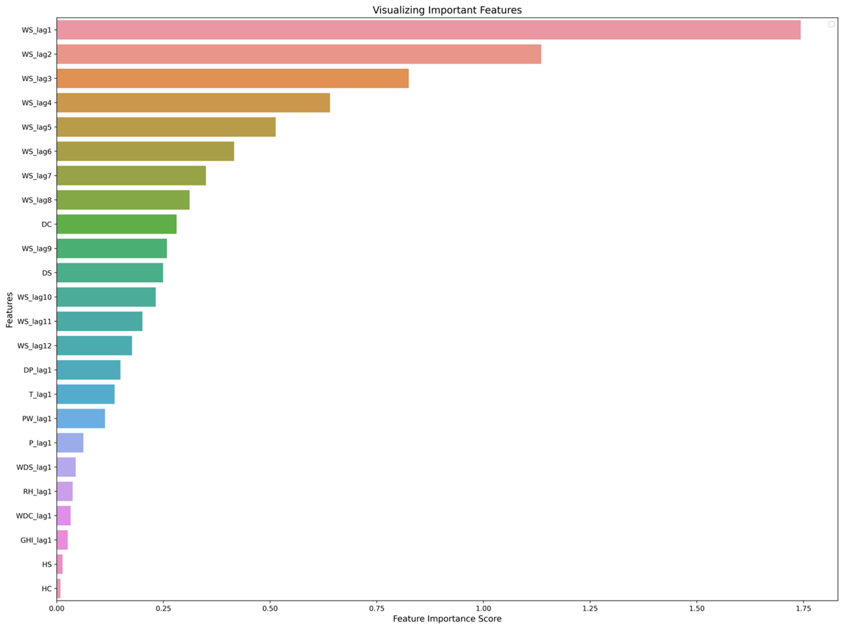
| Common Features | Caracas Only | Toronto Only | ||
|---|---|---|---|---|
| WS
(output) | T_lag1 | WS_lag1 | WS_1D | WS_lag8 |
| DP_lag1 | WS_lag2 | DNI_lag1 | WS_lag9 | |
| HS | RH_ lag1 | WS_lag3 | WS_lag10 | |
| HC | P_lag1 | WS_lag4 | WS_lag11 | |
| DS | PW_lag1 | WS_lag5 | WS_lag12 | |
| DC | WDS_lag1 | WS_lag6 | GHI_lag1 | |
| WDC_lag1 | WS_lag7 | |||
| Dataset | WS Mean | WS SD | WS VAR | WS MIN | WS MAX | |
|---|---|---|---|---|---|---|
| Alghat | Train: | 3.03 | 1.53 | 2.33 | 0.1 | 10 |
| Val: | 3.13 | 1.58 | 2.50 | 0.2 | 8.6 | |
| Test: | 3.01 | 1.43 | 2.04 | 0.2 | 9.2 | |
| All: | 3.04 | 1.52 | 2.31 | 0.1 | 10 | |
| Dumat Al Jandal | Train: | 2.65 | 1.40 | 1.97 | 0.1 | 9.8 |
| Val: | 2.79 | 1.55 | 2.39 | 0.1 | 10.3 | |
| Test: | 2.62 | 1.37 | 1.87 | 0.1 | 7.3 | |
| All: | 2.66 | 1.42 | 2.02 | 0.1 | 10.3 | |
| Waad Al Shamal | Train: | 3.08 | 1.56 | 2.44 | 0.2 | 10.6 |
| Val: | 3.40 | 1.69 | 2.86 | 0.4 | 11.1 | |
| Test: | 2.97 | 1.39 | 1.93 | 0.2 | 9.3 | |
| All: | 3.12 | 1.56 | 2.44 | 0.2 | 11.1 | |
| Yanbu | Train: | 3.17 | 1.61 | 2.58 | 0.1 | 11.2 |
| Val: | 3.31 | 1.70 | 2.89 | 0.1 | 9.9 | |
| Test: | 3.06 | 1.58 | 2.50 | 0.2 | 9.6 | |
| All: | 3.17 | 1.62 | 2.62 | 0.1 | 11.2 | |
| Caracas | Train: | 1.63 | 0.42 | 0.17 | 0.1 | 2.9 |
| Val: | 1.76 | 0.34 | 0.12 | 0.8 | 2.7 | |
| Test: | 1.39 | 0.39 | 0.15 | 0.1 | 2.6 | |
| All: | 1.62 | 0.42 | 0.17 | 0.1 | 2.9 | |
| Toronto | Train: | 4.38 | 2.37 | 5.60 | 0.1 | 14.7 |
| Val: | 3.85 | 2.49 | 6.17 | 0.3 | 15.6 | |
| Test: | 4.28 | 2.07 | 4.29 | 0.3 | 14.1 | |
| All: | 4.28 | 2.35 | 5.52 | 0.1 | 15.6 | |
| Hyperparameter | Value | Optimization |
|---|---|---|
| Learning Rate | 0.001 | Adam Optimizer |
| Number of Epochs | 100 | Activation Function = ReLU, Tanh * |
| Dropout | 0.1 | Loss Function = MSE |
| Batch Size | 500 | Early Stopping |
| Weight Decay | 0.000001 | Kernel Initializer = glorot uniform |
Disclaimer/Publisher’s Note: The statements, opinions and data contained in all publications are solely those of the individual author(s) and contributor(s) and not of MDPI and/or the editor(s). MDPI and/or the editor(s) disclaim responsibility for any injury to people or property resulting from any ideas, methods, instructions or products referred to in the content. |
© 2023 by the authors. Licensee MDPI, Basel, Switzerland. This article is an open access article distributed under the terms and conditions of the Creative Commons Attribution (CC BY) license (https://creativecommons.org/licenses/by/4.0/).
Share and Cite
Alkhayat, G.; Hasan, S.H.; Mehmood, R. A Hybrid Model of Variational Mode Decomposition and Long Short-Term Memory for Next-Hour Wind Speed Forecasting in a Hot Desert Climate. Sustainability 2023, 15, 16759. https://doi.org/10.3390/su152416759
Alkhayat G, Hasan SH, Mehmood R. A Hybrid Model of Variational Mode Decomposition and Long Short-Term Memory for Next-Hour Wind Speed Forecasting in a Hot Desert Climate. Sustainability. 2023; 15(24):16759. https://doi.org/10.3390/su152416759
Chicago/Turabian StyleAlkhayat, Ghadah, Syed Hamid Hasan, and Rashid Mehmood. 2023. "A Hybrid Model of Variational Mode Decomposition and Long Short-Term Memory for Next-Hour Wind Speed Forecasting in a Hot Desert Climate" Sustainability 15, no. 24: 16759. https://doi.org/10.3390/su152416759
APA StyleAlkhayat, G., Hasan, S. H., & Mehmood, R. (2023). A Hybrid Model of Variational Mode Decomposition and Long Short-Term Memory for Next-Hour Wind Speed Forecasting in a Hot Desert Climate. Sustainability, 15(24), 16759. https://doi.org/10.3390/su152416759