Data-Driven Chance-Constrained Schedule Optimization of Cascaded Hydropower and Photovoltaic Complementary Generation Systems for Shaving Peak Loads

Abstract

The coordinated scheduling of cascade hydropower with photovoltaic (PV) power stations can significantly improve the utilization rate of delivery transmission lines. However, the inherent uncertainty associated with photovoltaic (PV) forecasts challenges the reliable and economic operation of the complementary energy system. Against this background, in this paper, a day-ahead, chance-constrained scheduling for cascaded hydro–photovoltaic complementary generation systems (CHPSs) considering the transmission capacity is proposed. Firstly, the uncertainty of PV forecast errors is simulated by a probability density function fitted using kernel density estimation with historical sampling data. Then, a chance-constrained optimization model considering peak-shaving demands of the receiving-end power grid is developed to determine the day-ahead optimal schedules of CHPSs. Also, complex hydraulic coupling and unit operation constraints of cascade hydropower are considered in the proposed model. To deal with the nonlinear and stochastic constraints, an efficient linearization method is adopted to transform the proposed model into a mixed-integer linear programming (MILP) problem. Finally, the effectiveness and feasibility are verified by case studies. The results show that the day-ahead schedule optimized by the proposed method can fully balance peak-shaving and photovoltaic accommodation while considering photovoltaic output uncertainty.

1. Introduction

Overusing traditional fossil fuels has caused severe environmental pollution and accelerated the climate crisis in the last few decades. Replacing fossil fuels with renewable energy (RE), such as wind and photovoltaic (PV) sources, can alleviate this crisis to some extent. Against this background, the installed capacity and power generation of new energy sources, such as wind power and photovoltaic, continue to increase [1,2]. Due to the inherent intermittency, volatility, and uncertainty, the direct integration of wind power and photovoltaic creates challenges in the safe and stable operation of the power grid [3,4,5]. Combining flexible power resources (such as hydro and thermal) and renewable energy into a complementary power-generation system is an effective means to promote the consumption of new energy connected to the grid [6,7]. Among these options, hydropower generation is an environmentally friendly power source with the advantages of providing a fast response to load variability, robustness to weather fluctuations, and energy storage [8,9]. The coordination of hydropower and RE does not produce pollutants and contributes to sustainable society and economic growth with much lower carbon emissions. Thus, the coordination of hydropower and RE is preferred as a nonpolluting power source for replacing fossil fuels to alleviate the weather crisis and achieve cleaner and more sustainable energy systems. The insight is applicable for both large-scale and small-scale hydropower to offer sustainable development options for various conditions [10].

The coordination of the existing hydropower system with renewable energy in the river basin using the same delivery transmission lines to realize the bundled delivery of clean energy can effectively improve the utilization rate of the transmission channel and promote the accommodation of renewable energy, which is an important direction for the development and utilization of clean energy in the future [11,12,13]. There are many combinations of hydro–wind–photovoltaic hybrid systems that have been developed worldwide, especially in China, such as the wind-PV-hydro hybrid system located along the Yalong River and the hydro–photovoltaic hybrid system located at the Longyangxia hydropower station.

In recent years, research on the coordination of hydropower and complementary renewable energy scheduling has been widely discussed. Li et al. [14] proposed a long-term optimization model for the hydropower-PV hybrid system using multi-objective optimization programming, aiming to smooth the total power outputs and maximize the annual total power generation of the hybrid system at the same time. Silvério et al. [15] used floating PV plants to coordinate with hydropower plants, presenting a sizing optimization method considering technical and economical factors. Guo et al. [16] proposed a novel short-term operation model for a cascade hydro-PV complementary system using the artificial intelligence method, in which hybrid time steps are considered. Fagerström et al. [17] established an operation model for hydro-PV hybrid generation systems and investigated the potential of batteries to improve the cost-effectiveness of hydro-PV hybrid systems. The bundled transmission of hydro–wind–photovoltaic generation is inevitably constrained by the delivery transmission capacity. However, the above research does not analyze the influence of delivery transmission capacity on optimal dispatch. In addition, the operational status of units at the same hydropower station may differ simultaneously. Considering the possible variation of different units’ characteristics, the widely used plant-based hydropower operation model, in which the same energy conversion efficiency is applied for all units, may be inappropriate. Hence, extending plant-based to unit-based scheduling to obtain a more accurate model is necessary.

The output of renewable energy power generation is often difficult to predict accurately and has obvious uncertainty, which affects the economy and the security of the optimal scheduling of hydropower and renewable energy. Stochastic optimization is an effective method to deal with renewable energy power output uncertainty. Existing studies have extensively explored how to accurately generate the typical scenario set describing random factors. Lu et al. [18] presented a coordinated optimization mode for the hydropower-wind-PV hybrid system, where the uncertainties of predicted errors of wind and PV power outputs were formulated by scenarios generated using Latin hypercube sampling and k-means clustering. Zhang et al. [19] proposed several short-term scheduling optimization models with different dispatching preferences for operators. Forecasting based on probability functions was presented to obtain typical scenarios of random variables for the next dispatching horizon. Hu et al. [20] presented a day-ahead optimization model for the hybrid system consisting of cascaded hydropower, wind, and photovoltaic stations using the stochastic optimization method, where the strong regulation ability of hydropower is considered. To capture the correlation characteristics of wind and PV power, the improved generative adversarial networks method is adopted. Yuan et al. [21] proposed a coordination mechanism between the hydropower-PV co-generation station and the power grid. Guo et al. [22] proposed a generation curve formulation method to achieve steady power delivery considering the operation requirements of high-voltage direct current transmission. Representative scenarios were generated to describe the uncertainties of renewable energy power generation. Zhang et al. [23] proposed a stochastic optimization model for cascaded hydropower-wind PV plants, where the autoregressive moving average model and improved vine-copula theory are adopted to simulate the joint probability distribution of renewable energy power using measured data.

The above stochastic optimization models focus on generating typical scenarios to represent the wind and PV power uncertainties to balance the calculation speed and accuracy [24,25,26]. The key to these research papers is to generate a limited number of scenarios to represent the probability distribution characteristics of random variables. However, it is difficult to cover all possible scenarios, especially extreme scenarios, to analyze operation risks for multi-energy complementary systems. In the case of the limited transmission capacity of hydropower and photovoltaic systems, extreme PV output scenarios may influence the operation of the combined power generation system, resulting in severe renewable energy generation curtailment [27,28].

With the rapid development of the Chinese economy, the peak–valley differences of the power loads have tended to increase significantly. Since the ramping power of coal-fired thermal units is limited and requires several hours to start up or shut down, flexible power sources for peak regulation are obviously insufficient in a coal-dominated energy system, which increases operational costs and risks for power systems. Cascaded hydropower is characterized by huge installed capacities and flexible regulation capacity, usually applied for peak-shaving and frequency-regulating power systems.

Against this background, the peak-shaving operation of cascaded hydropower and photovoltaic generation systems (CHPSs) aims to smooth the residual load so that the residual power supplied by thermal units will be flat. However, the peak-shaving operation of CHPSs is a complex nonconvex and nonlinear programming problem because of the nonlinear formulation of hydropower production functions, spatial–temporal coupling of hydraulic connections, unit commitment constraints, and uncertainties associated with renewable energy generation [29].

In view of the above problems, this work aims to present a schedule-optimization model for the peak-shaving operation of CHPSs in which PV output uncertainty is involved based on a chance-constrained programming approach. Also, the complex constraints, including hydraulic connection, unit commitment, and limited transmission capacity, are considered. The main contributions of this paper can be summarized as follows:

(1)

A unit-based peak-shaving schedule optimization model for CHPSs considering transmission capacity is established in this paper. The proposed model considers the peak-shaving demand of the receiving-end power grid and the accommodation of PV power generation.

(2)

Non-parametric kernel density estimation is utilized to simulate probability density functions of PV forecast errors based on historical sampling data. To facilitate the modeling of PV uncertainties, the proposed schedule-optimization model is reformulated as a chance-constrained optimization. In addition, the proposed nonlinear model is transformed into a mixed-integer linear programming (MILP) problem to improve computational efficiency.

The remainder of the sections are organized as follows: Section 2 establishes the day-ahead coordination mechanism of cascaded hydropower plants and photovoltaic stations. Section 3 presents a peak-shaving schedule optimization model of cascade hydropower–wind–photovoltaic hybrid systems. Section 4 provides a chance-constrained reformulation and transformation of the proposed model. Case studies are carried out in Section 5, and conclusions are given in Section 6.

2. Day-Ahead Peak-Shaving Coordination for Cascade Hydropower and Photovoltaic Systems

Cascaded hydropower and photovoltaic complementary generation systems are shown in Figure 1. The cascaded hydropower station is bundled with a photovoltaic system to transmit power using the same transmission line to the receiving-end power system. The cascaded hydropower station can operate flexibly with good regulating ability, assisting in the creation of power-generation plans concerning the randomness and fluctuation of photovoltaic output.

The mode of CHPS participation in the power grid operation is as follows:

(1)

In the day-ahead stage, runoff data and photovoltaic outputs on the next day are predicted and reported to the centralized control center of CHPSs.

(2)

According to the forecast load data on the next day, the control center of CHPSs makes the unit commitment, stop, and generation plan of CHPSs, with the technical characteristics of cascaded hydropower such as water balance, power capacity, and start-up and shut-down operation constraints taken into account. The power output schedule of CHPSs is then submitted and reported to the system operator of the receiving-end system operator before the power delivery begins.

(3)

The system operator of the receiving-end power grids coordinates the power supply and loads of the whole power system to determine the final power generation curve of CHPSs. According to the confirmed transmission plan of CHPSs, the receiving-end system operator then arranges the generation plan for other power plants.

Therefore, the short-term peak-shaving model of CHPSs aims to decrease the peak-shaving pressure of the receiving-end power systems while considering the promotion of PV power. In the proposed model, the day-ahead output schedule of hydropower units, unit commitment schedule, and water discharge of the cascaded reservoir are optimized. However, PV power cannot be accurately predicted and is easily affected by meteorological factors such as radiation intensity. With limited transmission capacity, PV uncertainty may cause severe power curtailment. To cope with this issue, non-parametric kernel density estimation is utilized to fit the PV power forecast error, which is involved in the proposed schedule optimization model based on chance-constrained programming. Chance-constrained programming is useful for risk control when making decisions under uncertainties. By introducing the confidence parameters, chance constraints are established to ensure that any constraints subject to uncertainty factors will be feasible with a certain level of confidentiality predefined by the decision-makers. Using chance-constrained programming, PV uncertainty can be considered so that the PV power can be fully absorbed at a certain confidence level. It is important to highlight that this study has assumed that hydropower plants and photovoltaic stations are owned by the same stakeholder and operated by the same dispatching center, and thus cooperation between hydropower and photovoltaic power can be achieved smoothly.

3. Optimal Scheduling Model of CHPSs

3.1. Objective

The optimal scheduling of CHPSs aims to minimize the peak–valley difference of the receiving-end grid’s residual load. A scheduling optimization model of CHPSs is established to reduce the fluctuation of the residual load of the receiving-end power grid and reduce the regulating pressure of other peak-regulation sources (such as thermal power) [30]. The objective function can be expressed as follows:

$$\min F=\underset{t=1,2,\cdots ,T}{\max }{P}_{\mathrm{R},t}^{}-\underset{t=1,2,\cdots ,T}{\min }{P}_{\mathrm{R},t}^{}$$

(1)

$$P_{\mathrm{R},t}^{}=P_{\mathrm{L},t}^{}-P_{\mathrm{PV},t}-{\displaystyle \sum _{i=1}^I{\displaystyle \sum _{g=1}^{G_i}{P}_{i,g,t}}}$$

(2)

where $F$ is the peak–valley difference of the residual load of the receiving-end grid; $T$ is the number of periods in a scheduling cycle; $P_{\mathrm{R},t}^{}$ and $P_{\mathrm{L},t}^{}$ are the residual load and the original load of the receiving-end power grid at time interval $t$, respectively. $P_{\mathrm{PV},t}$ is the PV power output at time interval $t$, $I$ is the number of cascaded hydropower stations participating in operation, $G_i$ is the total number of units of hydropower station i, and $P_{i,g,t}$ is the output of unit $g$ in hydropower station $i$ at time interval $t$.

3.2. Constraints

• Water balance constraints:

$$V_{i,t}=V_{i,t-1}+\left(R_{i,t}^{}+Q_{i-1,t-{\tau }_{i-1}}^{\mathrm{out}}-Q_{i,t}^{\mathrm{out}}\right)\Delta t$$

(3)

$$Q_{i,t}^{\mathrm{out}}={\displaystyle \sum _{g=1}^{G_i}{q}_{i,g,t}}+s_{i,t}$$

(4)

where $V_{i,t}$ is the storage capacity of reservoir i at time interval $t$; $Q_{i,t}^{\mathrm{out}}$, $R_{i,t}^{}$, and $s_{i,t}$ are total water discharge, local inflow, and water spillage of hydropower station $i$ at time interval $t$, respectively; $q_{i,g,t}$ is the turbine discharge of unit $g$ in hydropower station $i$ at time interval $t$; $\Delta t$ indicates the duration of a scheduling period in the scheduling cycle; and ${\tau }_{i-1}$ is the water lag time between the hydropower station $i-1$ and hydropower station $i$. Water balance needs to be considered in the operation of a cascade hydropower system, as shown in (3) and (4).

2.

Storage control constraints:

$$V_{i,\min }^{}\le V_{i,t}^{}\le V_{i,\max }^{}$$

(5)

$$V_{i,0}^{}=V_{i,\mathrm{begin}}^{},V_{i,T}^{}=V_{i,\mathrm{end}}^{}$$

(6)

where $V_{i,\max }^{}$ and $V_{i,\min }^{}$ are the upper and lower limits of the storage capacity of reservoir $i$, respectively; and $V_{i,\mathrm{begin}}^{}$ and $V_{i,\mathrm{end}}^{}$ are the target control storage capacity of reservoir $i$ at the beginning and end of the dispatching period, respectively. Expressions (5) and (6) set the initial and expected terminal reservoir storage volumes, respectively.

3.

Power and abandoned water flow constraints:

$$u_{i,g,t}{q}_{i,g}^{\min }\le q_{i,g,t}\le u_{i,g,t}{q}_{i,g}^{\max }$$

(7)

$$0\le s_{i,t}\le s_{i,\max }^{}$$

(8)

where $u_{i,g,t}$ is a 0–1 variable representing the on–off state of unit $g$ in hydropower station $i$ at time interval $t$. If the unit is on, its value is 1; otherwise, it is 0. $q_{i,g}^{\max }$ and $q_{i,g}^{\min }$ are, respectively, the upper and lower limits of the generation flow of unit $g$ in hydropower station $i$; $s_{i,\max }^{}$ is the upper limit of abandoned water flow of hydropower station $i$. Expressions (7) and (8) give the upper and lower bounds of water discharge.

4.

Hydropower unit generation characteristic constraints:

Hydropower outputs can be expressed as a nonlinear function of turbine discharge, energy conversion ecoefficiency, and net water head, as shown in (9). Also, the upper and lower limits of hydropower outputs are shown in (10).

$$P_{i,g,t}=9.81\rho {\eta }_{i,g}{H}_{i,g,t}{q}_{i,g,t}$$

(9)

$$u_{i,g,t}{P}_{i,g}^{\min }\le P_{i,g,t}\le u_{i,g,t}{P}_{i,g}^{\max }$$

(10)

where $\rho$ is the density of water; ${\eta }_{i,g}$ is the generation efficiency of unit $g$ in hydropower station $i$; $H_{i,g,t}$ is the net water head of unit $g$ in hydropower station $i$ at time interval $t$; and $P_{i,g}^{\max }$ and $P_{i,g}^{\min }$ are, respectively, the maximum and minimum technical outputs of unit $g$ in hydropower station $i$.

5.

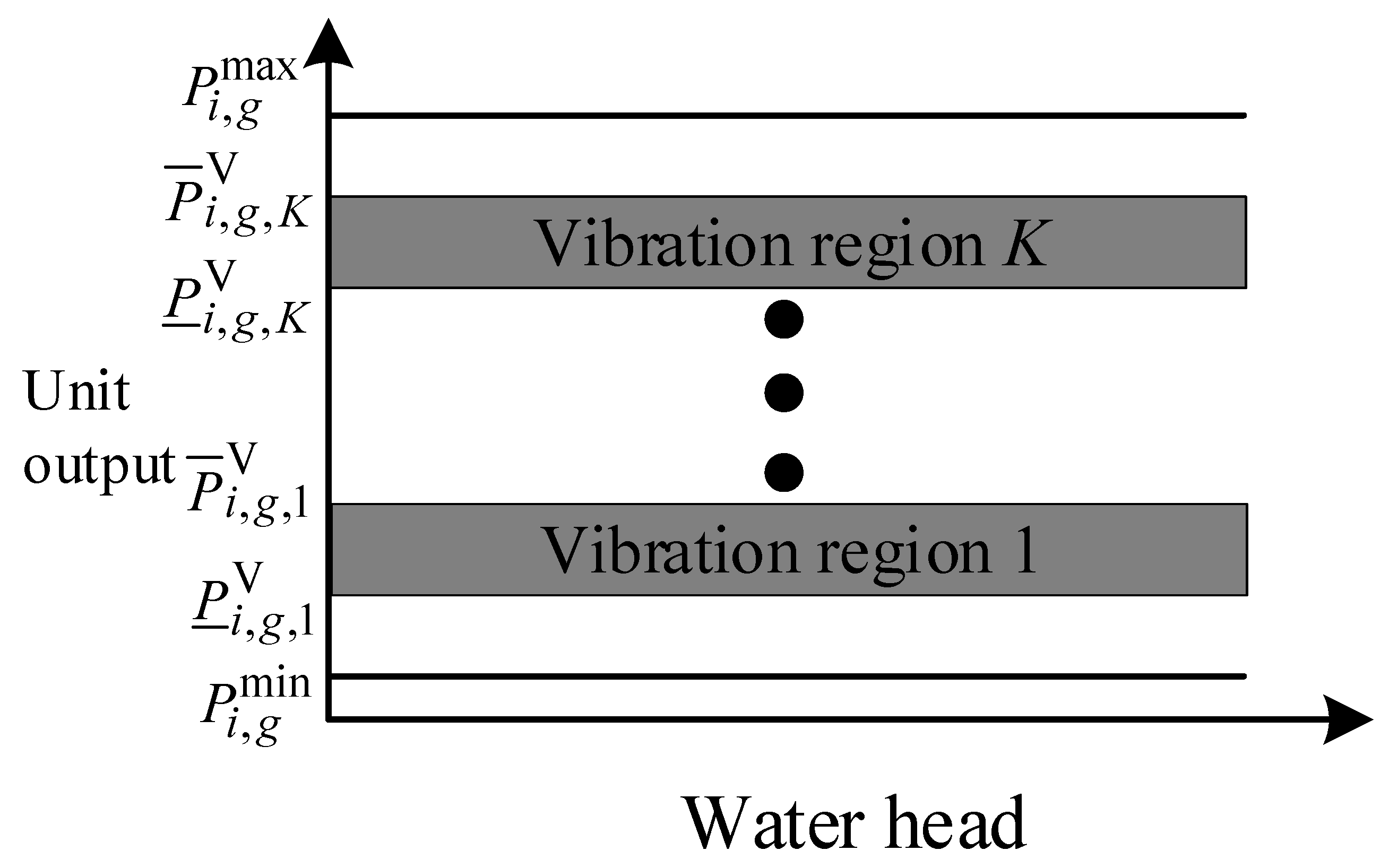
Vibration zone restriction of hydropower unit constraints:

Hydropower with a large capacity usually has several discontinuous vibration zones. Hydropower units should avoid operating in the vibration zones, as shown in (11).

$$\left(P_{i,g,t}-{\overline{P}}_{i,g,k}^{\mathrm{V}}\right)\left(P_{i,g,t}-{\underset{¯}{P}}_{i,g,k}^{\mathrm{V}}\right)\ge 0$$

(11)

where ${\overline{P}}^{\mathrm{V}}{}_{i,g,k}$ and ${\underset{\_}{P}}^{\mathrm{V}}{}_{i,g,k}$ are, respectively, the upper and lower limits of the vibration zone $k$ of unit g in hydropower station $i$.

6.

Unit commitment constraints:

$$\left\{\begin{array}{l}{y}_{i,g,t}-{\tilde{y}}_{i,g,t}=u_{i,g,t}-u_{i,g,t-1}\\ y_{i,g,t}+{\tilde{y}}_{i,g,t}\le 1\end{array}\right.$$

(12)

where $y_{i,g,t}$ and ${\tilde{y}}_{i,g,t}$ are 0–1 variables representing the start-up and shut-down operation of unit $g$ in hydropower station $i$ at time interval $t$, respectively. Expression (12) presents the relations of start-up and shut-down operations with on/off status for every hydropower unit.

7.

Generating head of the unit constraints:

$$H_{i,g,t}=\left(Z_{i,t}^{\mathrm{up}}+Z_{i,t-1}^{\mathrm{up}}\right)/2-Z_{i,t}^{\mathrm{tl}}-H_{i,g,t}^{\mathrm{loss}}$$

(13)

where $Z_{i,t}^{\mathrm{up}}$ is the forebay water level of reservoir $i$ at time interval $t$, $Z_{i,t}^{\mathrm{tl}}$ is the tail water level of reservoir $i$ at time interval $t$, and $H_{i,n,t}^{\mathrm{loss}}$ is the head loss of unit $g$ in hydropower station $i$ at time interval $t$. Expression (13) provides the calculation method of the net water head.

8.

Relation between forebay water level and reservoir storage capacity:

$$Z_{i,t}^{\mathrm{up}}=f_{\mathrm{FB},i}\left(V_{i,t}\right)$$

(14)

where $f_{\mathrm{FB},i}\left(\cdot \right)$ is the function of the forebay water level and storage capacity of reservoir $i$.

9.

Tail water–discharge relationship constraints:

$$Z_{i,t}^{\mathrm{tl}}=f_{\mathrm{TL},i}\left({\displaystyle \sum _{g=1}^{G_i}{q}_{i,g,t}}+s_{i,t}\right)$$

(15)

where $f_{\mathrm{TL},i}\left(\cdot \right)$ is a function of the tail water level of grade $i$ reservoir and the discharge flow.

10.

Delivery transmission capacity constraints:

The delivery transmission capacity of CHPSs is usually issued by the power system’s operator while considering the power system’s secure operation constraints. Then, the CHPS optimizes the schedule of hydropower and photovoltaic with the maximum transmission capacity as shown in (16):

$${\displaystyle \sum _{i=1}^I{\displaystyle \sum _{g=1}^{G_i}{P}_{i,g,t}}}+P_{\mathrm{PV},t}\le P_{\mathrm{L},\max }$$

(16)

where $P_{\mathrm{L},\max }$ is the maximum transmission capacity of transmission lines for CHPSs.

11.

Positive and negative system reserve constraints:

Hydropower stations usually assume the responsibility of providing reliable upward and downward reserves for power grids, which should be considered in the schedule optimization of CHPS, as shown in (17) and (18):

$${\displaystyle \sum }_{i=1}^I{\displaystyle \sum _{g=1}^{G_i}\left(u_{i,g,t}{P}_{i,g}^{\max }-P_{i,g,t}\right)}\ge \delta P_{\mathrm{L},t}$$

(17)

$${\displaystyle \sum }_{i=1}^I{\displaystyle \sum _{g=1}^{G_i}\left(P_{i,g,t}-u_{i,g,t}{P}_{i,g}^{\mathrm{m}\mathrm{in}}\right)}\ge \delta P_{\mathrm{L},t}$$

(18)

where $\delta$ is the load reserve rate required by receiving-end power grids.

In summary, the day-ahead optimal scheduling model of CHPSs comprises (1)–(18).

4. Chance-Constrained Model Formulation and Deterministic Transformation

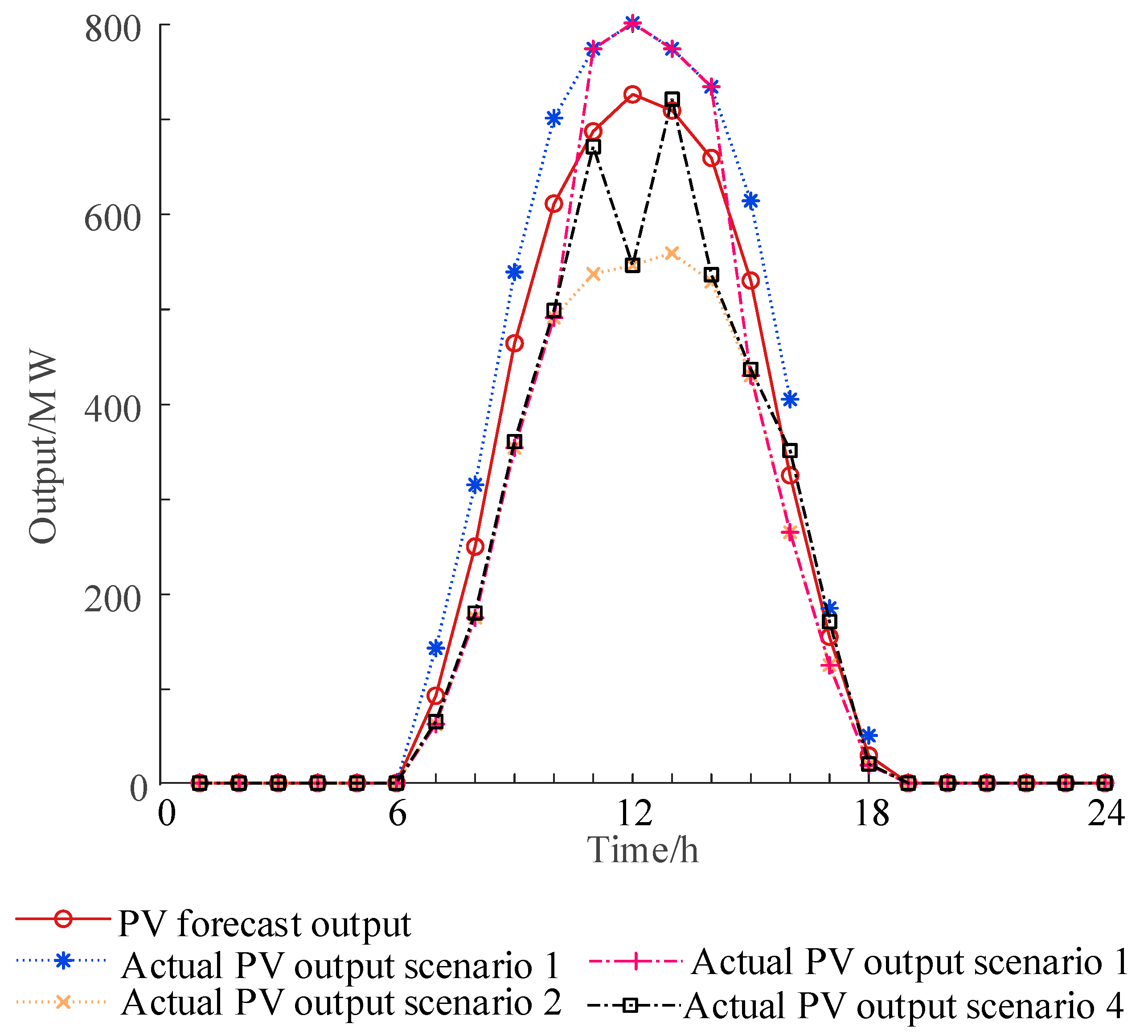
4.1. Modeling of PV Output Uncertainty Sets

In recent years, although PV power forecasting in the day-ahead has significantly improved, forecast errors of PV power generation are still unavoidable [31,32]. PV outputs are easily affected by weather, and PV output prediction has obvious uncertainty. The PV output can be described as the sum of the PV output predicted value and the PV prediction error, as shown in Equation (19):

$$P_{\mathrm{PV},t}=P_{\mathrm{PV},t}^{\mathrm{f}}+P_{\mathrm{PV},t}^{\mathrm{e}}$$

(19)

where $P_{\mathrm{PV},t}^{\mathrm{f}}$ is the predicted value of PV output at time interval $t$, and $P_{\mathrm{PV},t}^{\mathrm{e}}$ is the PV’s prediction error at time interval $t$. $P_{\mathrm{PV},t}^{\mathrm{f}}$ can be predicted in advance by combining meteorological information. $P_{\mathrm{PV},t}^{\mathrm{e}}$ has obvious uncertainty and fluctuates randomly within a certain range, which can be obtained based on experience or data analysis. Usually, the PV power forecast errors are assumed to follow a normal distribution to model the PV power uncertainty. However, it has been proven by many studies that the normal distribution can simulate the forecast error to a satisfying degree. With measured data, non-parametric kernel density estimation has good performance to estimate the probability distribution of random variables without relying on presetting probability distribution functions [33,34,35]. The kernel density estimation formulation for PV power output over a single time interval is shown in (20):

$$f_t(P_{\mathrm{PV},t}^{\mathrm{e}})=\frac{1}{n_t{h}_t}{\displaystyle \sum _{i=1}^{n_t}K(\frac{P_{\mathrm{PV},t}^{\mathrm{e}}-P_{\mathrm{PV},t,i}^{\mathrm{e}}}{h_t})}$$

(20)

where $n_t$ is the number of samples; $h_t$ is the bandwidth; $K(·)$ is the kernel density function, and the Gaussian kernel function is used in this paper; $P_{\mathrm{PV},t,i}^{\mathrm{e}}$ is the sample of forecast error that can be obtained from historical data of PV operation.

4.2. MILP-Based Formulation

The established model includes a min–max form objective function, as shown in (1); constraints with stochastic variables, as shown in (16); and non-linear constraints, as shown in (9), (11), (14), and (15), which make the proposed model difficult to solve directly. Many methods, such as Lagrangian relaxation (LR), dynamic programming (DP), and intelligent heuristic algorithms, have been applied to solve the hydropower scheduling-based problem. Many difficulties and challenges are encountered with the above methods [36]. In recent years, mixed-integer linear programming (MILP)-based approaches have been adopted by more and more researchers to solve hydropower scheduling-based problems because of the availability of better-performing and more user-friendly commercial software with efficient solvers such as CPLEX v12.10.0 and Gurobi v11.0 [37,38]. The various linearization methods can be used to transform the proposed model into a mixed-integer linear programming problem, as follows:

4.2.1. Transformation of the Objective Function

Since objective function (1) contains the nonlinear form of min–max, auxiliary variables $P_{\mathrm{R},\max }$ and $P_{\mathrm{R},\min }$ are first introduced to represent the maximum and minimum of the residual load of receiving-end power grids, and objective (1) is formulated as (21)–(23):

$$\min F=P_{\mathrm{R},\max }-P_{\mathrm{R},\min }$$

(21)

$$P_{\mathrm{R},\max }\ge P_{\mathrm{L},t}-{\displaystyle \sum _{i=1}^I{\displaystyle \sum _{g=1}^{G_i}{P}_{i,g,t}}}-P_{\mathrm{PV},t}^{\mathrm{f}}-P_{\mathrm{PV},t}^{\mathrm{e}}$$

(22)

$$P_{\mathrm{R},\min }\le P_{\mathrm{L},t}-{\displaystyle \sum _{i=1}^I{\displaystyle \sum _{g=1}^{G_i}{P}_{i,g,t}}}-P_{\mathrm{PV},t}^{\mathrm{f}}-P_{\mathrm{PV},t}^{\mathrm{e}}$$

(23)

where $P_{\mathrm{R},\max }$ and $P_{\mathrm{R},\min }$ are, respectively, the maximum and minimum value of residual loads of receiving-end power grids.

However, (22) and (23) contain the PV power output forecast error, which is a stochastic variable. The uncertainty of PV output makes it difficult to directly solve the model, and the equivalent transformation is required. To transform the proposed model into a deterministic one [36,37], the proposed objective can be further transformed into a chance constraint, as shown in (24)–(26):

$$\mathrm{Pr}\left\{P_{\mathrm{R},t,\min }^{\mathrm{C}}\le P_{\mathrm{L},t}-{\displaystyle \sum _{i=1}^I{\displaystyle \sum _{g=1}^{G_i}{P}_{i,g,t}}}-P_{\mathrm{PV},t}^{\mathrm{f}}-P_{\mathrm{PV},t}^{\mathrm{e}}\le P_{\mathrm{R},t,\max }^{\mathrm{C}}\right\}\ge \beta$$

(24)

$$P_{\mathrm{R},\max }\ge P_{\mathrm{R},t,\max }^{\mathrm{C}}$$

(25)

$$P_{\mathrm{R},\min }\le P_{\mathrm{R},t,\min }^{\mathrm{C}}$$

(26)

where $P_{\mathrm{R},t,\max }^{\mathrm{C}}$ and $P_{\mathrm{R},t,\min }^{\mathrm{C}}$ are, respectively, the lower and upper bounds of the interval of residual loads of receiving-end power grids at time interval t. (26) means that the residual load of receiving-end power grids is in the interval $\left[P_{\mathrm{R},t,\min }^{\mathrm{C}},P_{\mathrm{R},t,\max }^{\mathrm{C}}\right]$ at time interval t with the confidence level $\beta$.

The chance constraints make it difficult to solve directly. Using a cumulative probability distribution fitted by non-parametric kernel density estimation, chance-constraints are converted to the equivalent deterministic form as follows:

$$P_{\mathrm{L},t}-{\displaystyle \sum _{i=1}^I{\displaystyle \sum _{g=1}^{G_i}{P}_{i,g,t}}}-P_{\mathrm{PV},t}^{\mathrm{f}}-F_{\mathrm{PV},t}^{-1}(1-\beta )\le P_{\mathrm{R},t,\max }^{\mathrm{C}}$$

(27)

$$P_{\mathrm{L},t}-{\displaystyle \sum _{i=1}^I{\displaystyle \sum _{g=1}^{G_i}{P}_{i,g,t}}}-P_{\mathrm{PV},t}^{\mathrm{f}}-F_{\mathrm{PV},t}^{-1}(\beta )\ge P_{\mathrm{R},t,\min }^{\mathrm{C}}$$

(28)

where $F_{\mathrm{PV},t}^{-1}(·)$ is the inverse function of the cumulative density function of the PV forecast error at time interval t.

4.2.2. Transformation of Power Transmission Limits

Also, with the PV power forecast error, the power transmission limit constraint (16) contains a stochastic variable, which can be rewritten as (29). For the deterministic transformation of (29), the power transmission limit constraint can be formulated as the chance constraint, as expressed in (30) with the confidence level $\alpha$, and further transformed into a deterministic formulation using the cumulative density function, as shown in (31).

$${\displaystyle \sum _{i=1}^I{\displaystyle \sum _{g=1}^{G_i}{P}_{i,g,t}}}+P_{\mathrm{PV},t}^{\mathrm{f}}+P_{\mathrm{PV},t}^{\mathrm{e}}\le P_{\mathrm{L},\max }$$

(29)

$$\mathrm{Pr}\left\{{\displaystyle \sum _{i=1}^I{\displaystyle \sum _{g=1}^{G_i}{P}_{i,g,t}}}+P_{\mathrm{PV},t}^{\mathrm{f}}+P_{\mathrm{PV},t}^{\mathrm{e}}\le P_{\mathrm{L},\max }\right\}\ge \alpha$$

(30)

$${\displaystyle \sum _{i=1}^I{\displaystyle \sum _{g=1}^{G_i}{P}_{i,g,t}}}+P_{\mathrm{PV},t}^{\mathrm{f}}+F_{\mathrm{PV},t}^{-1}(\alpha )\le P_{\mathrm{L},\max }$$

(31)

4.2.3. Linearization of Output Characteristics of Hydropower Units

As seen in Equation (9), there is a nonlinear function relationship between hydropower unit outputs and the generating efficiency, generating flow, and generating water purification head. In this paper, it is assumed that the power-generation efficiency ${\eta }_{i,g}$ of each unit is constant, and the output characteristics of the hydropower unit can be linearized by the McCormick convex envelope relaxation method [20,39], as shown in (32)–(35).

$$P_{i,g,t}\ge \rho g{\eta }_{i,g}\left(q_{i,g}^{\min }{H}_{i,g,t}+H_i^{\min }{q}_{i,g,t}-q_{i,g}^{\min }{H}_i^{\min }\right)$$

(32)

$$P_{i,g,t}\ge \rho g{\eta }_{i,g}\left(q_{i,g}^{\max }{H}_{i,g,t}+H_i^{\max }{q}_{i,g,t}-q_{i,g}^{\max }{H}_i^{\max }\right)$$

(33)

$$P_{i,g,t}\le \rho g{\eta }_{i,g}\left(q_{i,g}^{\min }{H}_{i,g,t}+H_i^{\max }{q}_{i,g,t}-q_{i,g}^{\min }{H}_i^{\max }\right)$$

(34)

$$P_{i,g,t}\le \rho g{\eta }_{i,g}\left(q_{i,g}^{\max }{H}_{i,g,t}+H_i^{\min }{q}_{i,g,t}-q_{i,g}^{\max }{H}_i^{\min }\right)$$

(35)

4.2.4. Linearization of Vibration Zone Operation Constraints

The operation characteristics of a large hydropower unit are shown in Figure 2. There are usually multiple vibration zones within the feasible range of its technical output. The safe operation division of the unit is divided into several discontinuous zones [40,41], and the nonlinear constraint of Equation (11) is transformed into a linear constraint by introducing 0–1 variables, expressed as (36) and (37):

$${\displaystyle \sum _{k=1}^{K+1}{z}_{i,g,t}^k=u_{i,g,t}}$$

(36)

$${\displaystyle \sum _{k=1}^{K+1}{z}_{i,g,t}^k}{\underset{\_}{P}}_{i,g,k}^{}\le P_{i,g,t}\le {\displaystyle \sum _{k=1}^{K+1}{z}_{i,g,t}^k}{\overline{P}}_{i,g,k}^{}$$

(37)

where $K$ is the number of vibration zones of unit $g$ in hydropower station $i$, and $z_{i,g,t}^k$ is a binary variable. If the output of unit $g$ in hydropower station $i$ at time interval $t$ is located in the safe operation zone $k$, its value is 1; otherwise, it is 0. ${\overline{P}}_{i,g,k}^{}$ and ${\underset{\_}{P}}_{i,g,k}^{}$ are, respectively, the upper and lower limits of the safe operation zone $k$ of unit $g$ in hydropower station $i$. Their values correspond to the upper and lower limits of the vibration zone and the maximum and minimum technical output of the hydropower station, and the specific corresponding relationships are ${\underset{\_}{P}}_{i,g,1}^{}=P_{i,g}^{\min }$, ${\underset{\_}{P}}_{i,g,k+1}^{}={\overline{P}}_{i,g,k}^{\mathrm{V}}$, ${\overline{P}}_{i,g,k}^{}=$${\underset{¯}{P}}_{i,g,k}^{\mathrm{V}}$, and ${\overline{P}}_{i,g,K+1}^{}=P_{i,g}^{\max }$.

4.2.5. The Relationship between Forebay Water Level and Storage Capacity

The relationship between the forebay water level and the storage capacity is nonlinear. The nonlinear relationship is linearized by the piecewise linearization method, as shown in (38)–(42).

Firstly, the storage capacity of reservoir i is divided into $J$ intervals:

$$\left\{\begin{array}{l}{V}_i^{\min }=V_i^0<V_i^1<\cdots <V_i^j<\cdots <V_i^J=V_i^{\max }\\ Z_i^j=f_{\mathrm{FB},i}(V_i^j)\end{array}\right.$$

(38)

where $V_i^j$ is the water storage capacity of reservoir i at the endpoint of subdivision $j$, and $Z_i^j$ is the corresponding water level of reservoir $i$ at the endpoint of subdivision $j$. Then, at time interval $t$, the forebay water level $Z_{i,t}^{\mathrm{up}}$ and the storage capacity $V_{i,t}^j$ of reservoir $i$ can be expressed as (28)–(31):

$${\displaystyle \sum _{j=1}^J{r}_{i,t}^j}=1$$

(39)

$${\displaystyle \sum _{j=1}^J{V}_{i,t}^j}=V_{i,t}^{}$$

(40)

$$r_{i,t}^j{V}_i^{j-1}\le V_{i,t}^j\le r_{i,t}^j{V}_i^j$$

(41)

$$Z_{i,t}^{\mathrm{up}}={\displaystyle \sum _{j=1}^J\left\{r_{i,t}^j{Z}_i^{j-1}+\frac{Z_i^j-Z_i^{j-1}}{V_i^j-V_i^{j-1}}\cdot \left[V_{i,t}^j-r_{i,t}^j{V}_i^{j-1}\right]\right\}}$$

(42)

where $r_{i,t}^j$ is a binary variable to mark if the storage capacity of reservoir $i$ is in the section $j$ of storage capacity of at time interval $t$. If yes, it is 1; otherwise, it is 0.

4.2.6. Linearization of the Relationship between Tail Water Level and Release Flow

The relationship between tail water level and release water flow shown in Equation (15) is linearized by the piecewise linearization method similar to (38)–(42), which is not listed here.

To summarize, the day-ahead peak-shaving scheduling model proposed in this paper is converted into a MILP problem, which can be solved by a mature commercial solver. In this paper, the Yalmip/Gurobi solver solves the established optimal scheduling model.

5. Case Study

Three cascaded hydropower stations and one aggregated photovoltaic power station are included. The total installed capacity of the cascade hydropower station is 3310 MW, the capacity of the photovoltaic power station is 1000 MW, and the transmission capacity of the cascade hydropower system is limited to 3500 MW. Confidential levels $\alpha$ and $\beta$ are both set to 0.95. The predicted output value of the photovoltaic power station is shown in Figure 3. The upper and lower bounds of the actual output with the given confidence level (estimated using the inverse cumulative density function of the PV forecast error) are shown in Figure 3. The relevant parameters of cascade hydropower units, runoff, and reservoir parameters are shown in

Table 1. Parameters of cascaded hydropower units.

Hydropower Station	Installed Capacity/MW	Unit Vibration Zone/MW	Maximum Power Flow per Unit/(m3·s−1)
1	4 × 460	0~80, 150~300	257
2	4 × 300	0~40, 80~180	328

. The load curve of the receiving-end power grids takes the measured load of a power grid in a province of China as an example. The load peak value is 15,000 MW, the load valley value is 9600 MW, and the load peak–valley difference is 5400 MW.

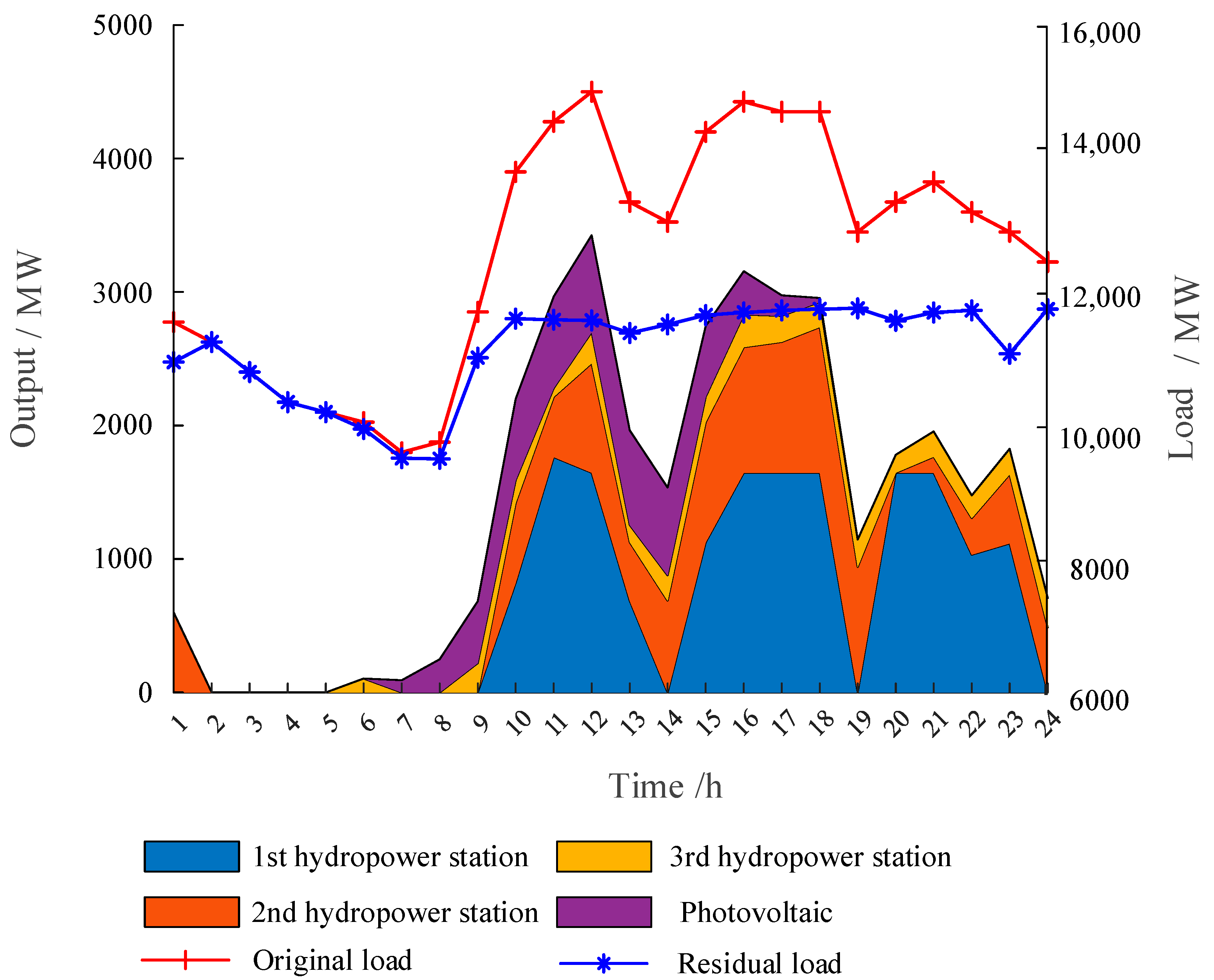
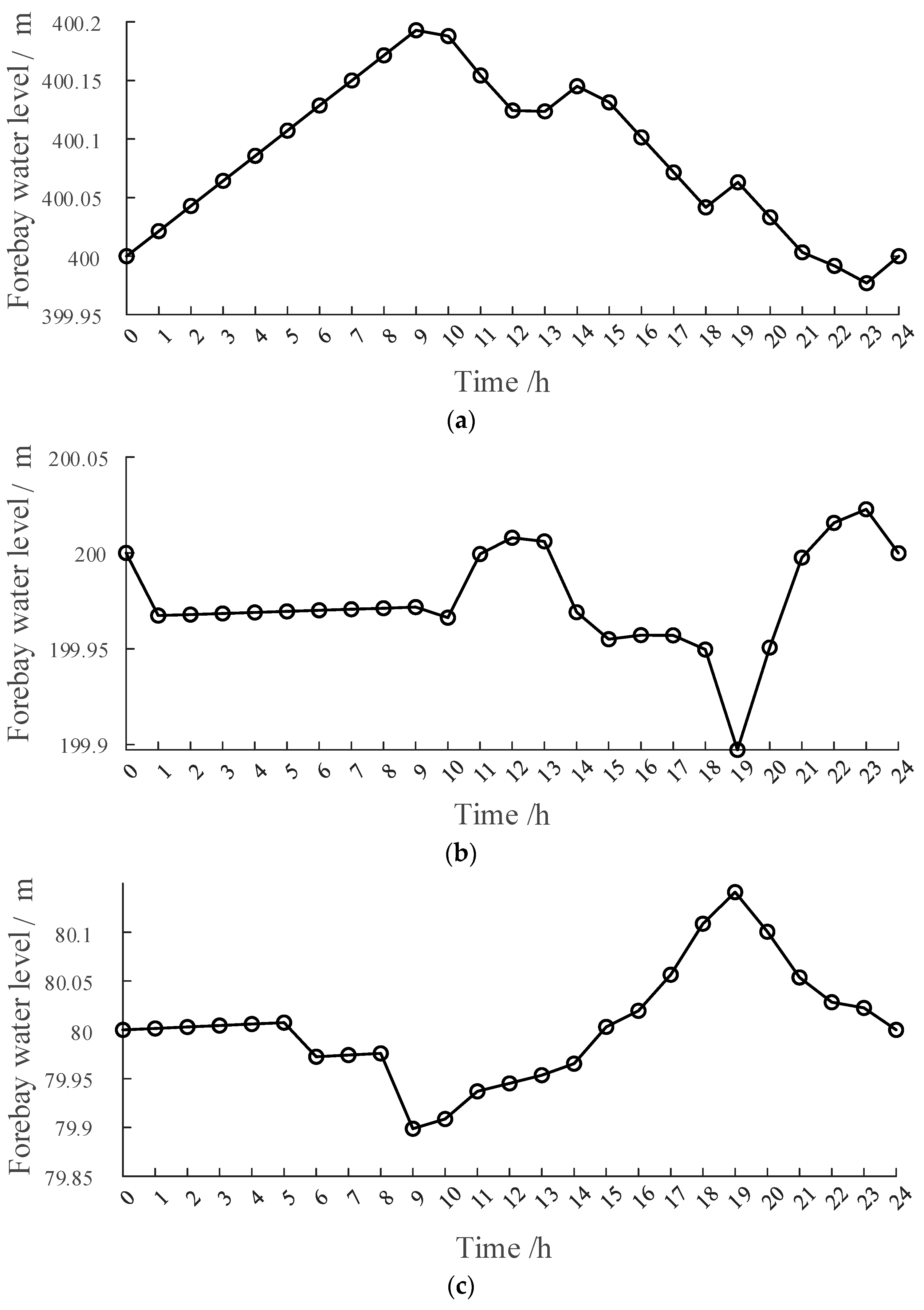
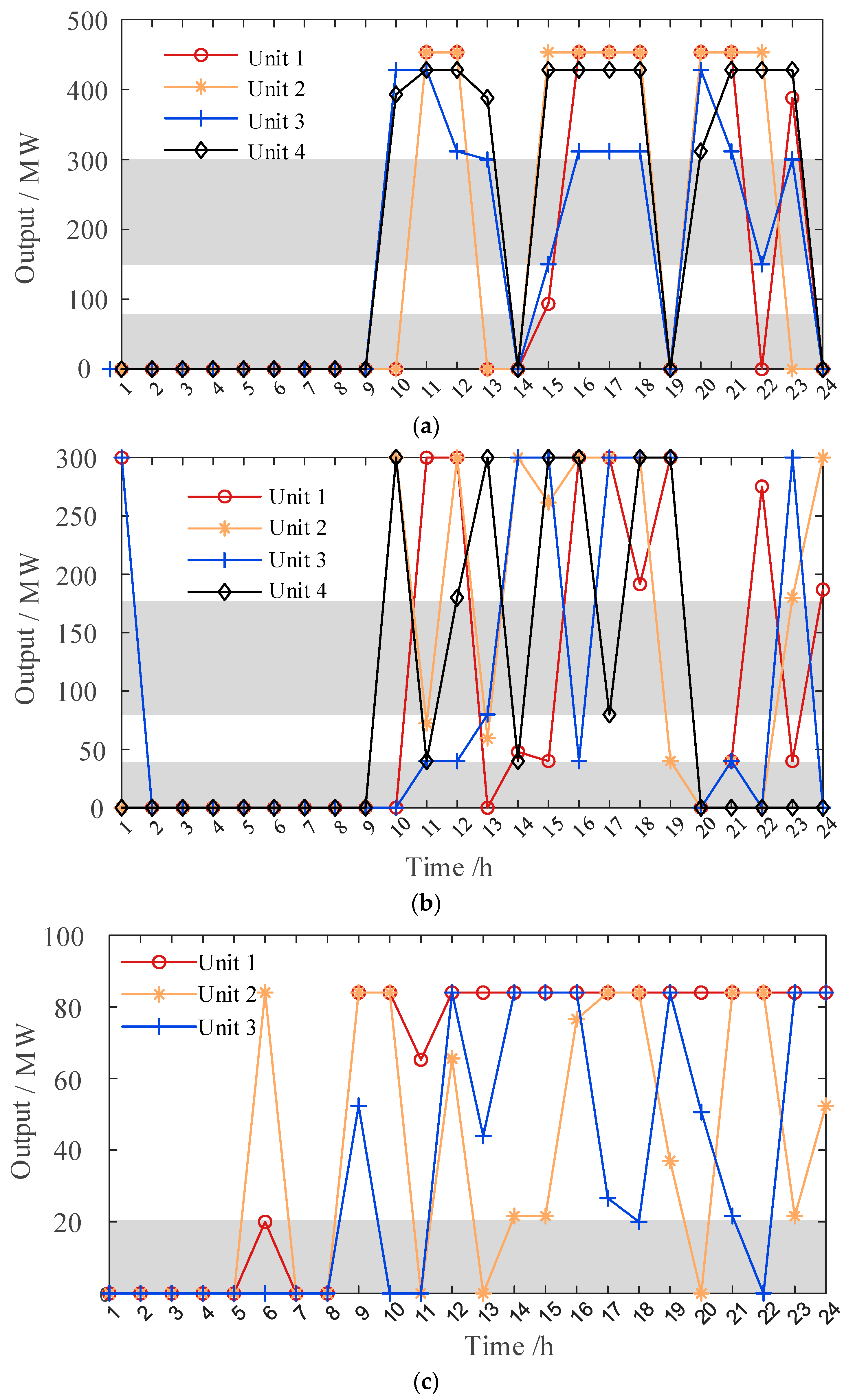
5.1. Analysis of the Results of Pre-Day Peak Scheduling

Figure 4 shows the optimized residual load curve of the receiving-end power grids and the output of hydropower and PV stations. Since PV outputs are uncertain, the PV outputs are the predicted values in Figure 4. It can be seen in Figure 4 that the CHPSs can adjust their power outputs according to the change in the load curve to achieve peak-shaving operation. The task of peak regulation is mainly undertaken by the first and second hydropower stations and the photovoltaic power station. This is because the reservoir capacity and installed capacity of the third hydropower station are small, and its regulation capacity is limited. In the valley load periods (1–7 h), the hydropower station stops and reduces its outputs. In the first load peak period (10–12 h), the photovoltaic outputs are high, and the cascade hydropower station appropriately reduces its outputs to ensure the full accommodation of photovoltaic power generation. In the second peak load period (16–18 h), the photovoltaic outputs decrease. The outputs of the cascaded hydropower station are increased to achieve the effect of peak regulation.

The peak-shaving effect of CHPSs on the grid is shown in

Table 2. Peak-shaving effect of proposed method.

Receiving-End Power Grids’ Load	Peak Value/MW	Valley Value/MW	Peak–Valley Difference/MW	Variance/MW2
Original load	15,000	9600	5400	3,022,344
Residual load	11,755	9436	2319	556,200

. As can be seen in Table 2, after the peak-shaving of CHPSs, the peak–valley difference of the receiving-end power grids’ load is reduced from the original 5400 MW to 2319 MW, with a decrease of 57.1%, and the load variance of the receiving-end power grids is reduced from 3,022,344 MW² to 556,200 MW², with a decrease of 81.6%. After the joint optimization of CHPSs, compared with the original load curve, the residual load curve is flatter, and the peak–valley difference and smoothness of the load curve are greatly improved. CHPSs can adjust their outputs in time according to the load-changing trend to meet the peak regulation demand of the receiving-end power grids and reduce the ramping and peak-shaving pressure of other regulating power sources in the receiving-end power grids.

Figure 5 shows the change curve of the forebay water level of cascaded hydropower over time on a dispatching horizon. It can be seen in Figure 5 that the forebay water level meets the upper and lower limits of the water level, and the water level at the end of the dispatching horizon meets the control requirements. Due to the valley load before 7 h, the first reservoir is continuously filled with water from 1 to 7 h to provide sufficient water storage for the subsequent peak-load periods to generate electricity for peak-shaving. The second hydropower station generates electricity at 1 h and carries out peak regulation for power grids, which results in a reduction in the water level of the second reservoir at this time. From 2 to 7 h, the second reservoir is continuously filled with water. The third-level reservoir will arrange the power-generation plan appropriately and reserve enough storage space for the subsequent period of operation. In the first peak-load periods, the PV outputs are high, and the peak load is mainly undertaken by the first-grade hydropower station. Therefore, the forebay water level of reservoir 1 decreases, while the forebay water level of the second-grade and third reservoirs increases due to the output limitation. In the second peak-load period, the PV outputs decrease, hydropower undertakes the main task of peak-load regulation, the first and second hydropower stations rapidly increase their outputs, and the forebay water level decreases. The first and second hydropower stations are multi-year and annually regulating power stations with large installed capacity and located upstream, which has a greater impact on the downstream inflow. The storage capacity of the third reservoir is small. The forebay water level of the third reservoir increases due to the significant increase in upstream inflow. After the second peak-load period, all forebay water levels of hydropower rationally arrange the output plan and finally reach the target control water level at the end of the dispatching horizon.

Figure 6 shows the on-off status and schedule plans of hydropower units. Since hydropower units can be flexibly started up and shut down, hydropower outputs are regulated to compensate for PV generation. In addition, with the constraints of vibration zones, hydropower can avoid all the vibration zones within a dispatching horizon.

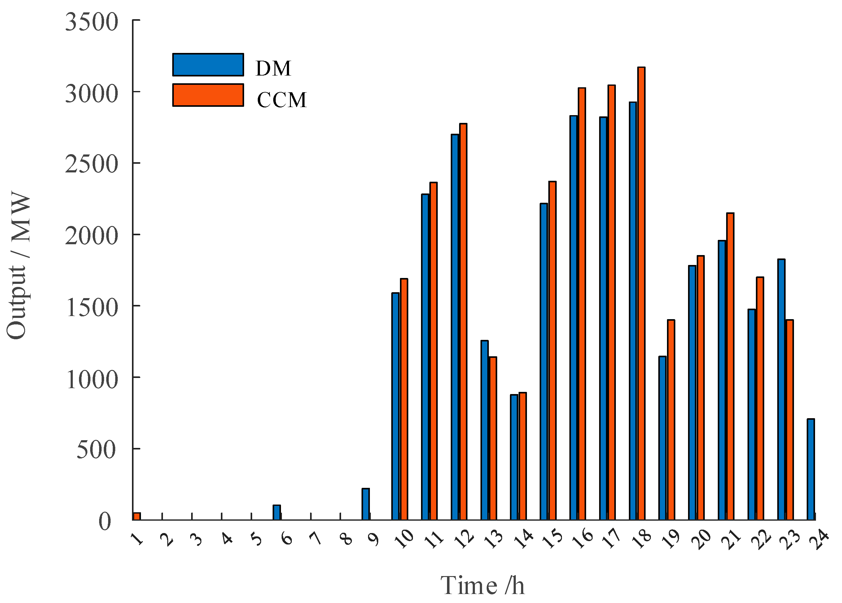
5.2. Comparison between Chance-Constrained Model and Deterministic Model

In order to illustrate the characteristics of the proposed chance-constrained model, the optimization results of the chance-constrained model (CCM) and the deterministic model (DM) are compared. The PV output in DM is equal to the predicted output. The cascade hydropower outputs obtained by CCM and DM when the delivery transmission capacity is limited to 3500 MW are compared, as shown in Figure 7. The cascade hydropower outputs obtained by CCM are slightly smaller than those obtained by DM during peak-load periods. This is because DM assumes that PV output is predicted accurately, and in order to achieve a maximum peak-shaving effect, scheduled outputs of hydropower in CHPSs reach the maximum delivery transmission capacity during peak-load periods. However, there is a certain overlap between the peak load period and the peak photovoltaic output period. In order to consider the uncertainty of PV output prediction, the output of hydropower in CHPSs obtained by CCM needs to leave a certain adjustment space for PV power generation by coordinating hydropower outputs when the delivery transmission capacity is limited. Therefore, during peak-load periods, cascade hydropower outputs obtained by CCM are reduced to avoid PV power abandonment in real-time operation due to the actual PV output being higher than the predicted output. Thus, the accommodation of PV power generation can be promoted.

Considering that the actual PV output fluctuates greatly, the actual peaking effect of CCM and DM in CHPSs is compared and analyzed, and typical PV actual output curves are selected within the given PV output fluctuation range, as shown in Figure 8. The peak-shaving effect obtained by CCM and DM in the actual PV output scenario is shown in

Table 3. Peak-shaving effect of different dispatching models.

Model	PV Output Scenario	Peak–Valley Difference/MW	PV Curtailment/(MW·h)
CCM	Predicted output	2074	0
	Scenario 1	2064
	Scenario 2	2217
	Scenario 3	2217
	Scenario 4	2219
DM	Predicted output	1999	0
	Scenario 1	2064	75
	Scenario 2	2142	0
	Scenario 3	2082	75
	Scenario 4	2145	0

. It can be seen in Table 3 that both CCM and DM models can reduce the peak load of receiving-end power grids by adjusting the output of cascade hydropower. The peaking effect of the cascade hydropower output plan obtained by CCM is slightly worse than that of DM in some scenarios, but CCM can consider the uncertainty of photovoltaic output to effectively avoid PV power generation abandonment. Therefore, the proposed CCM can improve the benefits of CHPSs while considering the demand for power grid peak regulation.

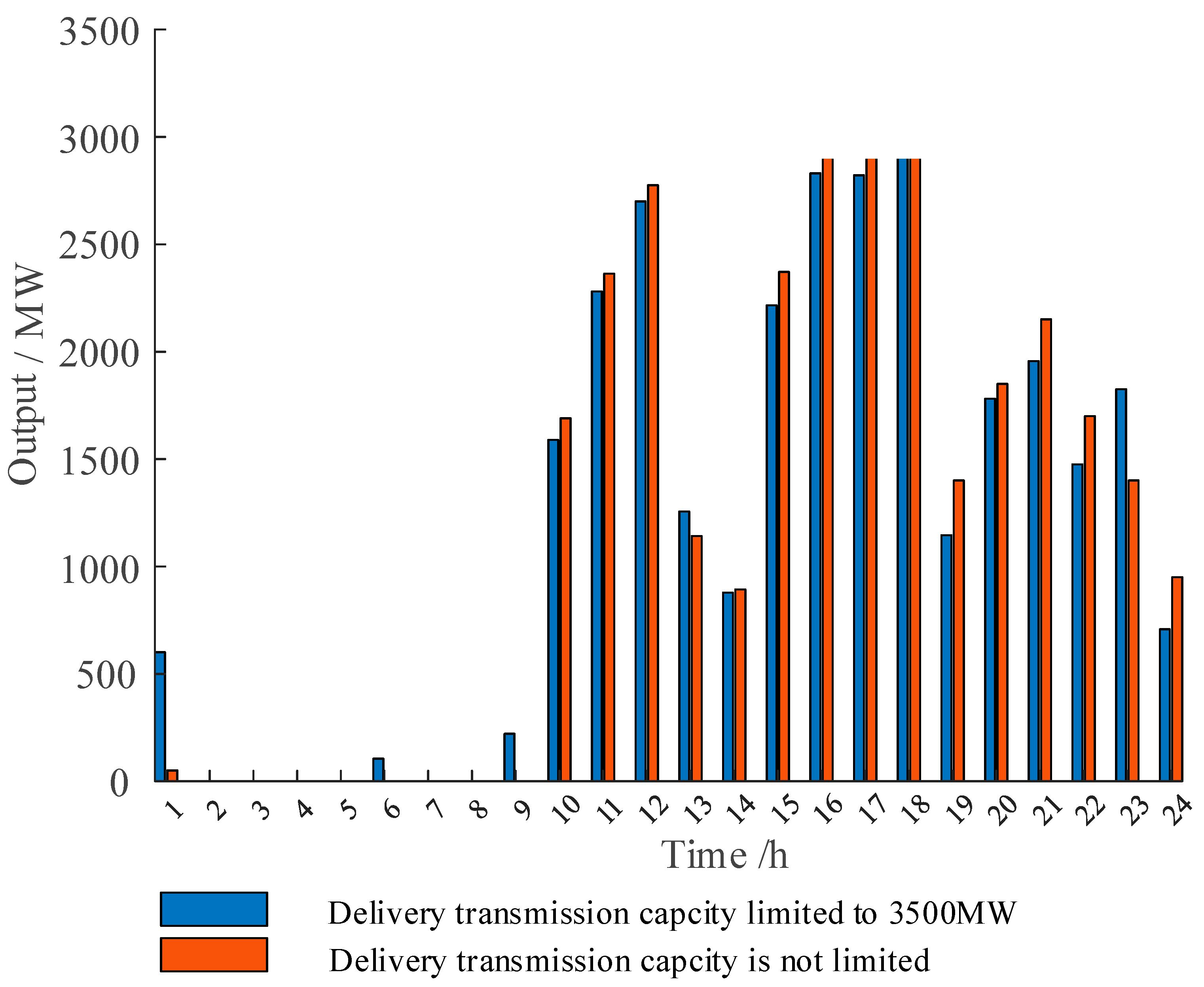
5.3. Sensitive Analysis of Delivery Transmission Capacity

The dispatching results of CHPSs will be affected by delivery transmission capacity. The peak-shaving effect of CHPSs under different delivery transmission capacities is shown in

Table 4. Peak-shaving results of different transmission capacities.

Delivery Transmission Line Capacity/MW	Peak Value/MW	Valley Value/MW	Difference between Peak and Valley/MW
3000	12,255	9436	2819
3300	11,955	9436	2519
3500	11,755	9436	2319
4000	11,554	9436	2118

. It should be pointed out that when the delivery transmission capacity is 4000 MW, the delivery transmission capacity is large enough relative to the installed capacity of hydropower and photovoltaic; that is, the hydropower and photovoltaic output is not limited by the delivery transmission capacity. In this case, the cascade hydropower output plan is the output plan that does not consider the delivery transmission capacity limit. As can be seen in Table 4, since the delivery transmission capacity will limit the hydropower output in CHPSs during peak-load periods, thus affecting the peak-shaving effect, with the increase in the delivery transmission capacity, the peak-shaving capacity of CHPSs will be enhanced, and the peak–valley difference of the receiving-end power grid will be reduced.

In order to analyze the influence of transmission capacity limitation on unit output, two cases are set up as follows:

• Case 1: delivery transmission capacity is 3500 MW;
• Case 2: delivery transmission capacity limits are not considered.

The day-ahead optimal schedule of cascade hydropower stations in two cases is shown in Figure 9. As can be seen in Figure 9, during peak-load periods, the cascade hydropower outputs of Case 2 are higher than those of Case 1. The reason for this result is that between 11 and 14 h, the actual PV output may be lower than the predicted output due to shielding and other reasons, thus reducing the peak-shaving effect of CHPSs during peak-load periods. Case 2 does not consider the limit of transmission capacity. Thus, in order to achieve a better peak-shaving effect under the worst PV output scenario, the CCM optimizes a cascade hydropower scheduling plan to increase hydropower outputs during this period to avoid deviation from the expected peak-shaving effect due to the decrease in PV output. In contrast, the hydropower-generation plan in Case 1 is low to avoid PV power generation abandonment due to the actual PV output being higher than the predicted output. The hydropower-generation plans of the two cases are different, and if the transmission capacity limit is not taken into account in operation, it will inevitably lead to serious energy abandonment.

The hydropower output plan and corresponding peak-shaving effect under different transmission capacity limits are different. Therefore, CHPSs need to fully consider the limitations of transmission capacity to formulate a reasonable scheduling plan. Then, the promotion of new energy accommodations and improvements in the peak-shaving effect can be balanced.

6. Conclusions

In this paper, a chance-constrained day-ahead peak-shaving scheduling optimization method for cascaded hydropower–photovoltaic complementary generation systems is proposed that considers the constraints of upstream and downstream hydraulic coupling and unit operation. The kernel density estimation is utilized to calculate the probability density functions of PV forecast errors. To deal with the proposed nonlinear and stochastic constraints in the proposed model, chance constraints are presented, and an efficient linearization method is proposed to transform the proposed model into a MILP problem. The effectiveness of the proposed model is verified by an example analysis. The numerical results show the following:

• By optimizing the power-generation schedule of cascaded hydropower stations, the fluctuation of photovoltaic power generation can be effectively compensated for, and the peak-shaving goal can be achieved. The output plan for cascaded hydropower is reasonable, with all the hydraulic and unit operation constraints satisfied.
• By fitting the PV forecast error with kernel density estimation, uncertainties of PV power outputs are included to formulate a chance-constrained optimization model for coordinating cascaded hydropower plants and PV stations. Using linear and deterministic transformations, the proposed chance-constrained model can be quickly solved by commercial software.
• The joint operation of hydropower and PV can effectively reduce the negative impact of PV power uncertainties on PV generation curtailment and peak-shaving capacity of CHPSs. That is, PV power curtailment is minimized while the demand for receiving-end power grids’ peak-shaving is satisfied.

With the development of renewable energy along with existing hydropower systems, bundled transmission using the same delivery transmission lines to deliver clean energy power is a promising pathway to improve the utilization of renewable energy. For an actual engineering project like the Longyangxia hydropower–PV complementary generation system, the proposed coordination method can be used to decrease the power curtailment caused by PV uncertainties. However, as hydropower uses its flexible regulation capacity to compensate for PV power, the coordination of hydropower and PV generation could damage the hydropower plant. In this work, a widely used assumption is made that hydropower plants and photovoltaic stations are owned by the same stakeholder and operated by the same dispatching center. In a practical project, hydropower and PV systems are not necessarily operated by the same operator. So, the coordination and compensation of hydropower and PV should be further investigated.

On the other hand, electricity markets have been widely established in China in recent years following the combination of medium- to long-term bilateral contracts and day-ahead spot transactions. In this case, the schedule optimization of CHPSs in electricity markets is of great significance and will be investigated in our further work. Specifically, two main challenges should be addressed: (1) balancing the transaction of medium- to long-term bilateral contracts and day-ahead sports markets, since these two markets are deeply coupled; and (2) quantifying and modeling uncertainties associated with renewable energy power and day-ahead market price.

References

1. Wang, C.; Hou, Y.; Qiu, F.; Lei, S.; Liu, K. Resilience enhancement with sequentially proactive operation strategies. IEEE Trans. Power Syst. 2017, 32, 2847–2857. [Google Scholar] [CrossRef]
2. Zhang, Y.Q.; Zang, W.; Zheng, J.H.; Cappietti, L.; Zhang, J.S.; Zheng, Y.; Fernandez-Rodriguez, E. The influence of waves propagating with the current on the wake of a tidal stream turbine. Appl. Energy 2021, 290, 116729. [Google Scholar] [CrossRef]
3. Wang, C.; Ju, P.; Lei, S.; Wang, Z.; Wu, F.; Hou, Y. Markov decision process-based resilience enhancement for distribution systems: An approximate dynamic programming approach. IEEE Trans. Smart Grid 2020, 11, 2498–2510. [Google Scholar] [CrossRef]
4. Zhang, Y.Q.; Zhang, Z.; Zheng, J.H.; Zheng, Y.; Zhang, J.S.; Liu, Z.Q.; Fernandez-Rodriguez, E. Research of the array spacing effect on wake interaction of tidal stream turbines. Ocean Eng. 2023, 276, 114227. [Google Scholar] [CrossRef]
5. Daneshvar, M.; Mohammadi-Ivatloo, B.; Abapour, M.; Asadi, S.; Khanjani, R. Distributionally robust chance-constrained transactive energy framework for coupled electrical and gas microgrids. IEEE Trans. Ind. Electron. 2021, 68, 347–357. [Google Scholar] [CrossRef]
6. Wang, Z.Z.; Wu, F.; Li, Y.; Li, J.Y.; Liu, Y.; Liu, W.E. Day-ahead dispatch approach for cascaded hydropower-photovoltaic complementary system based on two-stage robust optimization. Energy 2023, 265, 126145. [Google Scholar] [CrossRef]
7. Wang, Z.Z.; Wu, F.; Li, Y.; Shi, L.J.; Lee, K.Y.; Wu, J.W. Itô-theory-based multi-time scale dispatch approach for cascade hydropower-photovoltaic complementary system. Renew. Energy 2023, 202, 127–142. [Google Scholar] [CrossRef]
8. Avesani, D.; Galletti, A.; Piccolroaz, S.; Bellin, A.; Majone, B. A dual-layer MPI continuous large-scale hydrological model including human systems. Environ. Modell. Softw. 2021, 139, 105003. [Google Scholar] [CrossRef]
9. Anghileri, D.; Botter, M.; Castelletti, A.; Weigt, H.; Burlando, P. A comparative assessment of the impact of climate change and energy policies on alpine hydropower. Water Resour. Res. 2018, 54, 9144–9161. [Google Scholar] [CrossRef]
10. YoosefDoost, A.; Lubitz, W.D. Archimedes screw turbines: A sustainable development solution for green and renewable energy generation—A review of potential and design procedures. Sustainability 2020, 12, 7352. [Google Scholar] [CrossRef]
11. Zhang, Z.; Wu, X.; Liao, S.; Cheng, C. A ultra-short-term scheduling model for cascade hydropower regulated by multilevel dispatch centers suppressing wind power volatility. Int. J. Electric. Power Energy Syst. 2022, 134, 107467. [Google Scholar] [CrossRef]
12. Javed, M.S.; Ma, T.; Jurasz, J.; Amin, M.Y. Solar and wind power generation systems with pumped hydro storage: Review and future perspectives. Renew. Energy 2020, 148, 176–192. [Google Scholar] [CrossRef]
13. Irshad, A.S.; Samadi, W.K.; Fazli, A.M.; Noori, A.G.; Amin, A.S.; Zakir, M.N.; Bakhtyal, I.A.; Karimi, B.A.; Ludin, G.A.; Senjyu, T. Resilience and reliable integration of PV-wind and hydropower based 100% hybrid renewable energy system without any energy storage system for inaccessible area electrification. Energy 2023, 282, 128823. [Google Scholar] [CrossRef]
14. Li, F.; Qiu, J. Multi-objective optimization for integrated hydro-photovoltaic power system. Appl. Energy 2016, 167, 377–384. [Google Scholar] [CrossRef]
15. Silvério, N.M.; Barros, R.M.; Filho, G.L.T.; Redón-Santaf, M.; Santos, I.F.S.D.; Valério, V.E.D.M. Use of floating PV plants for coordinated operation with hydropower plants: Case study of the hydroelectric plants of the São Francisco River basin. Energy Convers. Manage. 2018, 171, 339–349. [Google Scholar] [CrossRef]
16. Guo, S.; Zheng, K.; He, Y.; Kurban, A. The artificial intelligence-assisted short-term optimal scheduling of a cascade hydro-photovoltaic complementary system with hybrid time steps. Renew. Energy 2023, 202, 1169–1189. [Google Scholar] [CrossRef]
17. Fagerström, J.; Das, S.; Klyve, Ø.S.; Olkkonen, V.; Marstein, E.S. Profitability of battery storage in hybrid hydropower–solar photovoltaic plants. J. Energy Storage 2024, 77, 109827. [Google Scholar] [CrossRef]
18. Lu, L.; Yuan, W.; Su, C.; Wang, P.; Cheng, C.; Yan, D.; Wu, Z. Optimization model for the short-term joint operation of a grid-connected wind-photovoltaic-hydro hybrid energy system with cascade hydropower plants. Energy Convers. Manage. 2021, 236, 114055. [Google Scholar] [CrossRef]
19. Zhang, Z.D.; Qin, H.; Li, J.; Liu, Y.Q.; Yao, L.Q.; Wang, Y.Q.; Wang, C.; Pei, S.Q.; Zhou, J.Z. Short-term optimal operation of wind-solar-hydro hybrid system considering uncertainties. Energy Conv. Manag. 2020, 205, 112405. [Google Scholar] [CrossRef]
20. Wei, H.; Zhang, H.X.; Yu, D.; Wang, Y.T.; Ling, D.; Ming, X. Short-term optimal operation of hydro-wind-solar hybrid system with improved generative adversarial networks. Appl. Energy 2019, 250, 389–403. [Google Scholar] [CrossRef]
21. Yuan, W.L.; Wang, X.Q.; Su, C.G.; Cheng, C.T.; Liu, Z.; Wu, Z.N. Stochastic optimization model for the short-term joint operation of photovoltaic power and hydropower plants based on chance-constrained programming. Energy 2021, 222, 119996. [Google Scholar] [CrossRef]
22. Guo, Y.; Ming, B.; Huang, Q.; Wang, Y.; Zhen, X.; Zhang, W. Risk-averse day-ahead generation scheduling of hydro–wind–photovoltaic complementary systems considering the steady requirement of power delivery. Appl. Energy 2022, 309, 118467. [Google Scholar] [CrossRef]
23. Zhang, H.; Lu, Z.; Hu, W.; Wang, Y.; Dong, L.; Zhang, J. Coordinated optimal operation of hydro-wind-solar integrated systems. Appl. Energy 2019, 242, 883–896. [Google Scholar] [CrossRef]
24. Jeong, C.; Furenes, B.; Sharma, R. Implementation of simplified sequential stochastic model predictive control for operation of hydropower system under uncertainty. Comput. Chem. Eng. 2023, 179, 108409. [Google Scholar] [CrossRef]
25. Sakki, G.K.; Tsoukalas, I.; Kossieris, P.; Makropoulos, C.; Efstratiadis, A. Stochastic simulation-optimization framework for the design and assessment of renewable energy systems under uncertainty. Renew. Sustain. Energy Rev. 2022, 168, 112886. [Google Scholar] [CrossRef]
26. Adhikari, A.; Jurado, F.; Naetiladdanon, S.; Sangswang, A.; Kamel, S.; Ebeed, M. Stochastic optimal power flow analysis of power system with renewable energy sources using adaptive lightning attachment procedure optimizer. Int. J. Electr. Power Energy Syst. 2023, 153, 109314. [Google Scholar] [CrossRef]
27. Nikoobakht, A.; Aghaei, J. Robust inter-reliant resilience of cyber-physical smart grids. Sustain. Energy Technol. Assess. 2023, 60, 103449. [Google Scholar] [CrossRef]
28. Zhang, Y.; An, X.; Wang, C. Data-driven two-stage stochastic optimization model for short-term hydro-thermal-wind coordination scheduling based on the dynamic extreme scenario set. Sustain. Energy Grids 2021, 27, 100489. [Google Scholar] [CrossRef]
29. Avesani, D.; Zanfei, A.; Marco, N.D.; Galletti, A.; Ravazzolo, F.; Righetti, M.; Majone, B. Short-term hydropower optimization driven by an innovative time-adapting econometric mode. Appl. Energy 2022, 310, 118510. [Google Scholar] [CrossRef]
30. Liao, S.; Liu, Z.; Liu, B.; Cheng, C.; Wu, X.; Zhao, Z. Daily peak shaving operation of cascade hydropower stations with sensitive hydraulic connections considering water delay time. Renew. Energy 2021, 169, 970–981. [Google Scholar] [CrossRef]
31. ElNozahy, M.S.; Salama, M.M.A. Uncertainty-based design of a bilayer distribution system for improved integration of PHEVs and PV arrays. IEEE Trans. Sustain. Energy 2015, 6, 659–674. [Google Scholar] [CrossRef]
32. Elazab, R.; Ser-Alkhatm, M.; Adma, M.A.A.; Abdel-Latif, K.M. A two-stage stochastic programming approach for planning of SVCs in PV microgrids under load and PV uncertainty considering PV inverters reactive power using Honey Badger algorithm. Electr. Power Syst. Res. 2024, 228, 109970. [Google Scholar] [CrossRef]
33. Xu, X.; Yan, Z.; Shahidehpour, M.; Li, Z.; Yan, M.; Kong, X. Data-driven risk-averse two-stage optimal stochastic scheduling of energy and reserve with correlated wind power. IEEE Trans. Sustain. Energy 2020, 11, 436–447. [Google Scholar] [CrossRef]
34. Liu, B.; Lund, J.R.; Liao, S.; Jin, X.; Liu, L.; Cheng, C. Peak shaving model for coordinated hydro-wind-solar system serving local and multiple receiving power grids via HVDC transmission lines. IEEE Access 2020, 8, 60689–60703. [Google Scholar] [CrossRef]
35. Liu, B.; Lund, J.R.; Liao, S.; Jin, X.; Liu, L.; Cheng, X. Optimal power peak shaving using hydropower to complement wind and solar power uncertainty. Energy Convers. Manage. 2020, 209, 112628. [Google Scholar] [CrossRef]
36. Guisández, I.; Pérez-Díaz, J.I. Mixed integer linear programming formulations for the hydro production function in a unit-based short-term scheduling problem. Energy Syst. 2021, 128, 106747. [Google Scholar] [CrossRef]
37. Connolly, D.; Lund, H.; Finn, P.; Mathiesen, B.V.; Leahy, M. Practical operation strategies for pumped hydroelectric energy storage (PHES) utilising electricity price arbitrage. Energy Policy 2011, 39, 4189–4196. [Google Scholar] [CrossRef]
38. Finardi, E.C.; Takigawa, F.Y.K.; Brito, B.H. Assessing solution quality and computational performance in the hydro unit commitment problem considering different mathematical programming approaches. Electr. Power Syst. Res. 2016, 136, 212–222. [Google Scholar] [CrossRef]
39. Apostolopoulou, D.; Greve, Z.D.; Mcculloch, M. Robust optimization for hydroelectric system operation under uncertainty. IEEE Trans. Power Syst. 2018, 33, 3337–3348. [Google Scholar] [CrossRef]
40. Yuan, W.; Xin, W.; Su, C.; Cheng, C.; Yan, D.; Wu, Z. Cross-regional integrated transmission of wind power and pumped-storage hydropower considering the peak shaving demands of multiple power grids. Renew. Energy 2022, 190, 1112–1126. [Google Scholar] [CrossRef]
41. Zhang, J.; Cheng, C.; Yu, S.; Su, H. Chance-constrained co-optimization for day-ahead generation and reserve scheduling of cascade hydropower variable renewable energy hybrid systems. Appl. Energy 2022, 324, 119732. [Google Scholar] [CrossRef]
Figure 1. Schematic diagram of cascaded hydropower and photovoltaic complementary generation system.
Sustainability 15 16916 g001
Figure 2. Schematic diagram of vibration zone of hydropower units.
Sustainability 15 16916 g002
Figure 3. Fluctuation range of photovoltaic output.
Sustainability 15 16916 g003
Figure 4. Optimal dispatching results of CHPSs.
Sustainability 15 16916 g004
Figure 5. Water level curves of cascaded reservoirs. (a) The first hydropower station; (b) The second hydropower station; (c) The third hydropower station.
Sustainability 15 16916 g005
Figure 6. Hydropower outputs of different units. (a) The first hydropower station; (b) The second hydropower station; (c) The third hydropower station.
Sustainability 15 16916 g006
Figure 7. Comparison of hydropower output between DM and CCM.
Sustainability 15 16916 g007
Figure 8. Photovoltaic power-generation output.
Sustainability 15 16916 g008
Figure 9. Cascaded hydropower output comparison of different transmission capacities.
Sustainability 15 16916 g009