Determining the Appropriate Minimum Effort Levels for Use in Fisheries Dynamic Bioeconomic Models

Abstract

Managing fisheries to achieve ecological, economic and social sustainability is complex. The use of dynamic bioeconomic models can be and have been used to assist in determining management targets. However, optimizing profits over time can result in large reductions in fishing effort in the short term with adverse social consequences. There exist other benefits from maintaining fishing effort even in adverse conditions (e.g., maintain crew and fleet capacity). For this reason, many bioeconomic models have included some form of minimum effort, catch or short-term profit constraint. In this paper, we consider a range of approaches to assess an appropriate minimum fishing effort, including the estimation of fishery breakeven effort levels, and approaches based on historical fishing levels. These are tested using a bioeconomic model currently used for fishery management. We find that breakeven approaches tend to result in the most conservative effort levels and the highest net present value of profits. In contrast, using a proportion of the moving average of the observed fishing effort results in less conservative change in effort, while resulting in positive changes in the net present value of fishery profits. The approach also has the advantage of being dynamic, adjusting with recent fishery conditions.

1. Introduction

Fishery management is generally implemented to achieve multiple objectives [1]. Foremost of these is the ecological sustainability of the resource, but more recently fishery management has embraced a number of economic and social objectives [2,3]. Identifying appropriate harvest or effort levels given such an objective mix is complex, and a range of fishery bioeconomic models have evolved to assist in this process. Bioeconomic models generally capture explicitly the economic and ecological sustainability aspects of management, as the two objectives are largely complementary. However, social aspects are more difficult to incorporate, as often they are difficult to identify and measure, and the relationship between stock conditions and their achievement is often obfuscated. For example, the achievement of some social objective may parallel achievement of economic and ecological sustainability objectives, while other social objectives may be achieved only at the cost of fully achieving economic and ecological objectives. For others still, there may be no apparent relationship between the different objectives.

The use of bioeconomic models to assist in fishery management has other challenges. A feature of many dynamic bioeconomic models of fisheries is their propensity to operate at only two levels, with zero harvest being applied while stocks build to their optimal level and then fish at this optimal level from that point onwards—the so-called bang-bang solution to fishery management [4,5,6]. While mathematically appealing, such solutions are impractical from a management perspective, and may not even be desirable from an economic and social perspective. Larkin et al. [7] identified a range of reasons not to close a fishery for a period to allow stocks to recover to an optimal level if closure can be avoided. These include benefits associated with continued data collection, especially as (in the absence of fisheries independent data) fishing allows the stock to be monitored as it recovers; support for coastal communities that may be dependent on the fishery and unable to withstand a period of closure; retaining experienced labour in the harvest and/or post-harvest sectors; and maintaining markets that may be lost to imports or other producers [7].

To avoid zero or extremely low catch or effort being estimated by the model, and thereby avoid the loss of potential social and some economic outcomes, minimum effort levels are often imposed in dynamic bioeconomic models [8,9,10,11,12,13,14]. Other models have addressed this through imposing a minimum total allowable catch each year [15]. The concept of co-viability and the associated development of co-viability models in fisheries also generally impose minimum acceptable levels of activity that bound the co-viability space [16]. Co-viability analysis in fisheries often include minimum effort [16] or minimum profitability (i.e., non negative or higher) constraints [17,18].

While imposing a non-negative profit constraint as a minimum has an economic logic and the condition is readily identifiable, other constraints may be equally desirable in recognition of the supplementary benefits identified by Larkin et al. [7]. Identifying the appropriate level of a minimum effort or catch constraints to achieve these benefits is less discernible. In many cases, these are based on what is considered an acceptable minimum level of effort by industry [11].

Such has been the case in Australia’s Northern Prawn Fishery, an effort-controlled fishery managed with the objective of achieving the maximum economic yield (MEY). The fishery is a multispecies prawn fishery with three sub-fisheries that are temporally and spatially separate (but overlap to some degree). The (common) banana prawn fishery operates in the first half of the year, and is managed primarily using a trigger catch rate aimed at preventing effort exceeding levels where the marginal cost exceeds the marginal benefit [19]. The tiger prawn fishery operates in the second half of the year and involves two tiger prawn and two endeavour prawn species (plus other species caught as byproduct). The third fishery—the redleg banana prawn fishery—also operates in the second half of the year, although is geographically separate to the tiger prawn fishery. Fishing effort, however, can move between the fisheries depending on relative catch rates and economic conditions. Fishing effort required to achieve MEY in the redleg banana prawn fishery is assessed using a discrete population dynamics model and proxy biomass-based target reference points for MEY (i.e., B_MEY, the biomass of the stock at MEY).

Of interest in this study is the model that has been developed to estimate MEY in the tiger prawn fishery. A bioeconomic model has been used to determine the effort trajectory that achieves MEY, defined as the trajectory that maximizes the net present value of the fishery over a 40-year period, and achieves a sustainable yield in seven or fewer years [10]. The model is run bi-annually with an integrated stock assessment and the first two years of the derived effort trajectory are used to set the total allowable effort (TAE) for the next two years [19].

The bioeconomic model incorporates a minimum fishing effort imposed at the request of industry [19] to ensure the fleet remains economically and socially viable in each year and the longer term, given the market and skilled labour retention benefits noted by Larkin et al. [7]. The bioeconomic model has been used to set management targets since the fishery undertook a major restructuring in 2007, with the need for a minimum effort level identified prior to the 2009 assessment [20]. In May 2008, the Resource Assessment Group (RAG)—a management advisory group consisting of scientists, managers and industry, determined that the model would use “a new minimum value of half the 2007 tiger prawn effort and an 8% efficiency increase” [20]. The 2007 tiger prawn effort was 5142 days, giving a new minimum effort level of 2777 days. However, as there are two tiger prawn species in the model that can be targeted separately to some extent (with endeavour prawns caught as by product in both), the minimum of 2777 days was applied to each species. This gives a total minimum level of fishing effort of 5554 days, allocated equally between the two fishing activities, which has since become embedded in the fishery’s harvest strategies [19,21].

In the 2022 stock assessment, the use of this minimum resulted in a recommended TAE higher than the observed level of fishing effort in the previous year, despite indications of a decline in stock. This raised concerns about its validity: the minimum constraints became binding at too high a level of effort given the stock status and adversely influenced the model outcomes. Instead, an ad hoc effort level based on a 10–20% cut in effort (as nominal days) relative to the recent five-year average was recommended as the TAE [22].

The aim of this paper is to explore different potential minimum effort levels based on several alternative approaches and assess how these may impact the outcomes of the bioeconomic model. While results are specific to the Northern Prawn Fishery bioeconomic model, the approaches may be applicable to other fisheries elsewhere confronting similar issues.

2. Materials and Methods

Two general approaches were adopted to assess a suitable minimum effort level for the fishery: (1) an economic approach based on the effort level required to at least break even; and (2) a “pragmatic” approach based on a proportion of historic fishing effort levels.

2.1. Definition of Key Concepts

The approaches use several economic concepts that may be unfamiliar to non-economists. These are defined below:

• Revenue is the value of the catch (price times quantity);
• Variable costs are the costs directly related to the level of fishing activity and catch (e.g., fuel, crew costs, freight and packaging);
• Fixed costs are the costs that are incurred independently of the level of fishing activity (e.g., management levies, insurance, accountancy, boat maintenance, etc.);
• Net revenue is revenue minus variable costs;
• Profits are revenue minus both fixed and variable costs;
• The breakeven level of effort is the minimum number of fishing days (and the associated net revenue) required for profits to be greater than or equal to zero.

2.2. Breakeven Analysis

The fishery is multi-species, with most boats operating in the banana prawn component of the fishery before the start of the tiger prawn fishery. The banana prawn fishery fluctuates substantially from year to year, driven largely by environmental variability [23,24]. As the banana prawn fishery precedes the tiger prawn fishery, the revenue from the tiger prawn fishery (net of variable costs) required to break even over the year, and hence the level of fishing effort required to achieve this net revenue, is dependent also on the net revenue derived from the banana prawn season.

An economic survey is conducted annually by the industry association (Northern Prawn Fishery Industry Pty Ltd., NPFI, Queensland, Australia) to provide input into the bioeconomic model as well as other management instruments (e.g., the banana prawn MEY trigger). The survey provides average costs and earnings from a sample of around 30–35 boats (out of a possible 52). From this, we derived an estimate of the number of days required to operate in the tiger prawn fishery for the vessels to break even on average over the year. We used data from 2007 to 2022. While earlier data were available, the fishery went through a major restructure in 2006 so that the cost structure in earlier years may not be representative of the current fleet.

The approach is undertaken in two stages. The first stage estimated the additional net revenue required from the tiger prawn fishery on average to break even for the year, while the second stage estimates how many days fishing is required to achieve this level of net revenue given prices, costs and stock conditions in each year. The net revenue required from the tiger prawn fishery for each boat ($N{R}_T$), on average, to break even is equivalent to the shortfall in vessel profits if there is no effort applied in the tiger prawn fishery. That is, revenue is only obtained from the banana prawn fishery, from which variable costs related to fishing in the banana prawn fishery and fixed costs are deducted:

$$N{R}_T=\min \left\{\left(C_B\left[p_B(1-c)-m\right]-(f_B+R{M}_B)D_B-F\right),0\right\},$$

(1)

where F is the average fixed cost per vessel ($/vessel), $C_B$ is the average catch of banana prawns per vessel over the season (kg), $p_B$ is the average price of banana prawns ($/kg), c is the crew share of revenue (%), m is the market, packaging and freight cost per kilogram of catch ($/kg), $f_B$ is the average fuel cost per day fished for banana prawns ($/day), $R{M}_B$ is the average repairs and maintenance cost per day fished and $D_B$ is the average number of days fished for banana prawns. In a “good” year in terms of banana prawn catch, the net revenue from the banana prawn fishery may exceed the fixed costs, in which case the fishery may not require any additional effort in the tiger prawn fishery to break even, and the required net revenue is zero. In other years, the net profit from fishing only for banana prawns will be negative.

Given the net revenue required to break even from the tiger prawn fishery, the average number of days required is estimated by

$$D_T=\left|N{R}_T\right|/\left[C_T\left[p_T(1-c)-m\right]-(f_T+R{M}_T)\right],$$

(2)

where $D_T$ is the average number of days required to break even fishing for tiger and endeavour prawns, $C_T$ is the average catch of tiger and endeavour prawns per vessel per day over the season (kg/day), $p_T$ is the average price of tiger and endeavour prawns ($/kg), $f_T$ is the average fuel cost per day fished for tiger prawns ($/day), and $R{M}_T$ is the average repairs and maintenance cost per day fished.

The breakeven number of days estimated using Equation (2) were used in two additional steps. First, we derived the distribution of the empirically based breakeven effort levels over the last 16 years and estimated the threshold values that are likely to be applicable at different levels of certainty, e.g., 50%, 60% or 80% based on previous prices and costs. Second, we applied econometric modelling to estimate the effects of factors that influence this level, such as prices and fuel costs. This may enable a “dynamic” threshold to be determined based on the best available information.

2.3. Historic Effort Levels

Three “pragmatic” approaches were also considered. The first was to consider the use of a proportion (e.g., 50%, 75%, 80%, etc.) of the moving average of actual fishing effort over a particular period (e.g., 3 or 5 years). This has no underlying rationale other than it is easy to estimate, and the shorter period (3 years) moving average reflects more recent conditions in the fishery.

The second approach was to consider the minimum level of fishing effort observed in the fishery since the restructure in 2007. The underlying rationale for this is that fishers have previously accepted not fishing beyond this point as an appropriate response to the prevailing stock and economic conditions.

The final approach involved using regression analysis to model the supply of fishing effort as a function of catch, catch rates and prices, with the intercept representing a minimum effort level in the absence of variable incentives to increase or decrease this level.

2.4. Testing the Different Threshold Effort Levels Using the Bioeconomic Model

The effect of the different minimum effort levels on the bioeconomic model outcomes was tested under two different conditions (models). The stock assessment model and settings used for 2018 estimated that the fishery was in relatively good condition from both a biological and economic perspective. Conversely, reductions in the stock of the key tiger prawn species and increased fuel costs in 2022 resulted in the stock assessment model producing contradictory results, with the minimum effort level forcing the “recommended” effort level to be higher than the previous year’s (2021) observed level, despite the more adverse economic and biological conditions.

The potential minimum effort levels based on the breakeven and more pragmatic approaches were applied to both models, and the outcomes compared against the observed level of fishing effort in each of the two years (reflecting fisher behaviour given the actual conditions experienced).

3. Results

3.1. Breakeven Analysis

3.1.1. Analysis of Cost and Earnings Data

The average profit per boat from fishing only for banana prawns (i.e., assuming zero tiger prawn fishing effort and net revenue) was estimated for the period 2007 to 2022. Missing data for 2009 resulted in an estimate not being available for this year. In five of the 15 years, the net revenue (i.e., revenue less variable fishing costs) from the banana prawn fishery was sufficient to cover all fixed costs, such that no additional fishing effort (and associated net revenue) was required to break even. That is, the profit in these years was positive even without additional net revenue from tiger prawn fishing. The profit from just the banana prawn fishery (excluding net revenue from the tiger prawn fishery) in each year and the banana prawn revenue in that year is shown in Figure 1. Given that this outcome is largely driven by the level of revenue from the banana prawn fishery, there is a moderate relationship between the level of banana prawn revenue and the profit assuming zero tiger prawn fishing, shown by the red dashed line. This relationship, however, is not strong (R² = 0.36), indicating that other factors, particularly fishing costs, are also driving the level of profit that can be derived from the banana fishery on its own.

The number of days per vessel (on average) required to breakeven in this case was estimated using Equation (2), based on the observed net revenue per day from tiger prawn fishing from the economic survey. This was expanded to the fleet level to derive an estimate of the minimum number of days required for the tiger fishery as a whole to break even. As this depended on conditions in the tiger prawn fishery as well as the banana prawn fishery, the relationship between this value and banana prawn revenue was relatively weak (Figure 2).

As indicated in Figure 1, zero tiger prawn fishing effort (and associated net revenue) was required in five of the years (33% of the observations) as all costs (i.e., variable costs associated with banana prawn fishing and vessel fixed costs) were fully covered by the banana prawn fishery. Also shown in Figure 2 is the maximum level of effort in the tiger prawn fishery over the period of the data. For one of the years (2020), effort in excess of this maximum would have been required to break even. For another two of the years (2011, 2022), no feasible levels of fishing effort would have resulted in the fishery breaking even as the average net revenue from tiger fishing per day was estimated to be negative from the survey data (that is, the average revenue per day from tiger prawn fishing was less than the average variable costs of fishing). Consequently, all three years (2011, 2020 and 2022) were recorded as making a loss in the economic survey.

Apart from those three years for which the fishery was unable to make a profit, the breakeven level of effort was lower than the current minimum effort threshold used in the model. Further, the current minimum effort threshold is 92% of the maximum observed level of effort (Figure 2). A general downward linear relationship between the number of tiger prawn fishery days needed to break even and the banana prawn revenue was observed (blue dashed line), although again this relationship was weak (as shown by the R² value) due to the number of zero days and also the number of infeasible days.

A cumulative probability distribution was derived from the breakeven effort data (Figure 3). From the economic survey data, 20% of the years made a loss over the period of the data. That is, the fishery may be only expected to break even 80% of the time given the observed maximum level of fishing effort available to the fleet. This can also be achieved with lower levels of fishing effort, roughly 4000 boat days. Similarly, no tiger prawn fishing is required 33% of the time to break even (as seen by the y-axis intercept). From Figure 3, the threshold effort value to achieve a given probability of breakeven profits (e.g., 50%) can be derived.

3.1.2. Breakeven Regression Analysis

Given that the breakeven effort level varies substantially from year to year, regression analysis was undertaken to determine what factors may influence this level. As approximately one third of the estimated breakeven effort levels were zero, standard regression models are not appropriate, and alternative estimation procedures were considered. A censored Tobit model was initially tested, but the coefficients were generally not significant, or the wrong sign given a priori expectations (e.g., the breakeven point decreased with increased fuel cost counter to expectations).

A zero-inflated negative binomial count model was also tested. This is a two-part model. First, a logistic (i.e., logit) model is applied to estimate the probability of an observation being either a zero or a non-negative outcome; then, a “normal” negative binomial count model is applied to the non-negative component. The models were estimated using the pscl package [25] in R [26]. The output from the model provides information on both components, the first part being the output relating to the “normal” negative binomial count model, and the second component relating to the probability that a value is zero. The key variables available for the model included the banana prawn revenue, fuel costs and tiger prawn prices. The latter was found to be not significant in both parts of the model.

The final model (based on the Akaike Information Criterion, or AIC) is given in

Table 1. Zero inflated negative binomial count model.

	Estimate	Std. Error	Significance
Count model coefficients (negative binomial with log link):
Intercept	7.013	0.271	***
Banana Prawn Revenue ($’000)	−0.005	0.000	**
Fuel cost per day ($’000)	0.484	0.000	**
Log(theta)	1.984	0.120	***
Zero-inflation model coefficients (binomial with logit link):
Intercept	−1.812	2.914
Fuel cost per day ($’000)	0.928	1.775
Theta (dispersion parameter)	7.27
Log-likelihood on 6 Df	−64.29
AIC	140.58

Significance codes: ‘***’ 0.001 ‘**’ 0.01 ‘*’ 0.05 ‘.’ 0.1 ‘ ’ 1.

. The estimation of the zero inflated negative binomial count model does not produce a standard goodness of fit measure. However, the predicted values of the dependent variable were reasonably correlated (given the existence of the zero levels) with the observed levels (r = 0.608), suggesting that the model reasonably captures the general trend in the data.

As expected, the breakeven effort level decreased with increasing banana prawn revenue, and increased with fuel costs (as the net tiger prawn revenue per day would decrease, requiring more days to achieve the required breakeven level of profit). While the variables in the zero-inflation model were not significant, excluding this component resulted in a less well-fitting model (as given by the log likelihood and the AIC).

As the variables in the model are logged, the coefficients also represent elasticities (i.e., the percentage change in breaking even given a 1% change in the variable being considered). While the elasticity relating to banana prawn revenue is small, this is a highly variable value, with a coefficient of variation of 37%. The breakeven number of days is also sensitive to changes in fuel costs, with a 1% change in fuel costs resulting in almost a 0.5% change in the breakeven effort level. The base level breakeven point is given by the exponential of the constant, estimated as 1670 nominal boat days.

The predicted breakeven level of effort, derived from the count model coefficients, fluctuated between 2000 and 3000 boat days a year (Figure 4) in the first half of the data (i.e., prior to 2014), although it was below 2000 boat days between 2014 and 2020. The probability of zero days being required to break even, derived from the zero-inflation model coefficients, was also highest between 2016 and 2020 but decreased to its lowest level in 2022 (Figure 4).

3.2. Historic Effort Levels

Three-year and five-year moving averages were derived from the available fishing effort time series [27] over the period 2007 to 2022, and different proportions were considered for testing using the bioeconomic model (

Table 2. Potential threshold effort levels based on historic effort data.

	3-Year Moving Average		5-Year Moving Average
	2018	2022	2018	2022
Percentage of moving average
80%	4241	3612	4316	3951
60%	3181	2709	3237	2963
50%	2651	2258	2698	2469
Minimum observed (2007–2022)	3599

). The minimum observed in the fishery over this period was also considered (Table 2).

The fishing effort time series was also regressed against the available economic information. Several different functional forms of the model were estimated. The most appropriate included a measure of average net revenue (fishing revenue less fuel costs) per day in the tiger prawn component of the fishery (

Table 3. Nominal fishing effort regression model.

	Estimate	Std. Error	Significance
Intercept	8.103	0.118	***
Log (Revenue less fuel cost per day, tiger prawn fishery)	0.217	0.061	**
$R^2$	0.471
${\overline{R}}^2$	0.433
$F_{\left(1,14\right)}$	12.49		***

Significance codes: ‘***’ 0.001 ‘**’ 0.01 ‘*’ 0.05 ‘.’ 0.1 ‘ ’ 1.

). As expected, total fishing effort over the year increased with an increasing average net revenue per day (Figure 5).

As with the breakeven point model, the minimum level of fishing effort that might be expected is given by the exponential of the constant, estimated as 3305 nominal boat days. The coefficient on the net revenue term also represents the effort elasticity, with a 1 percent increase in average net revenue in the tiger prawn fishery resulting in a 0.2% increase in total days fished over the season.

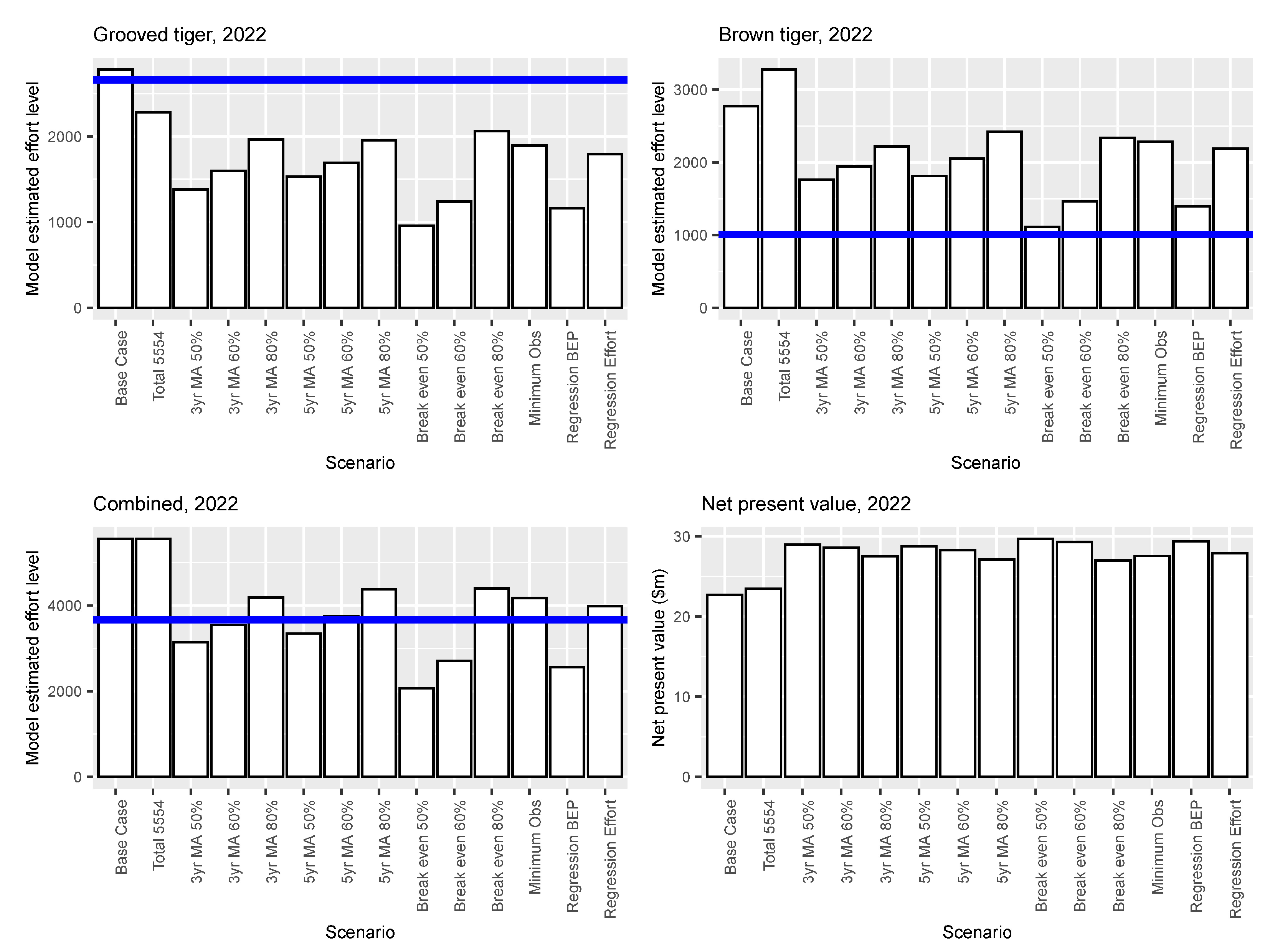
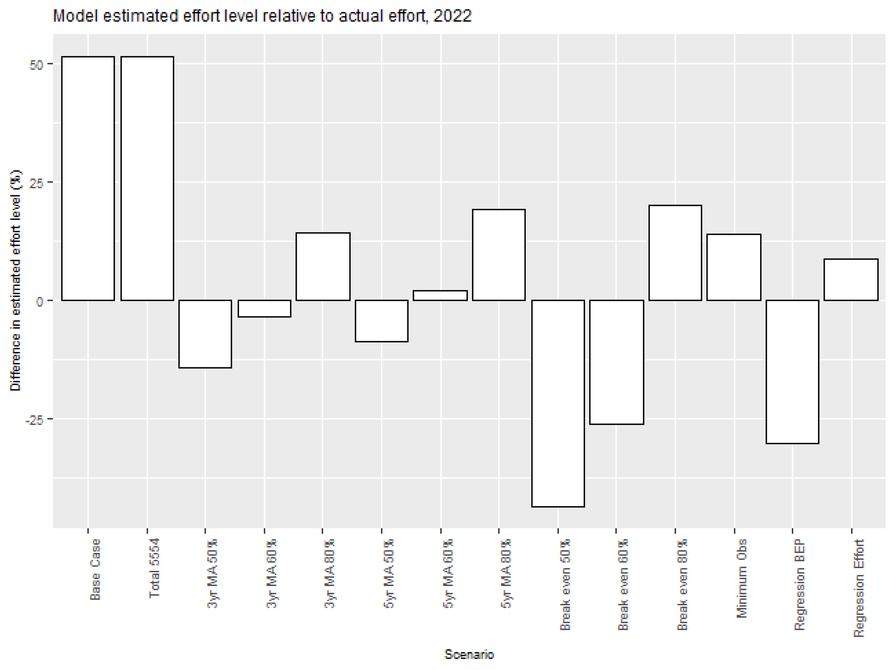
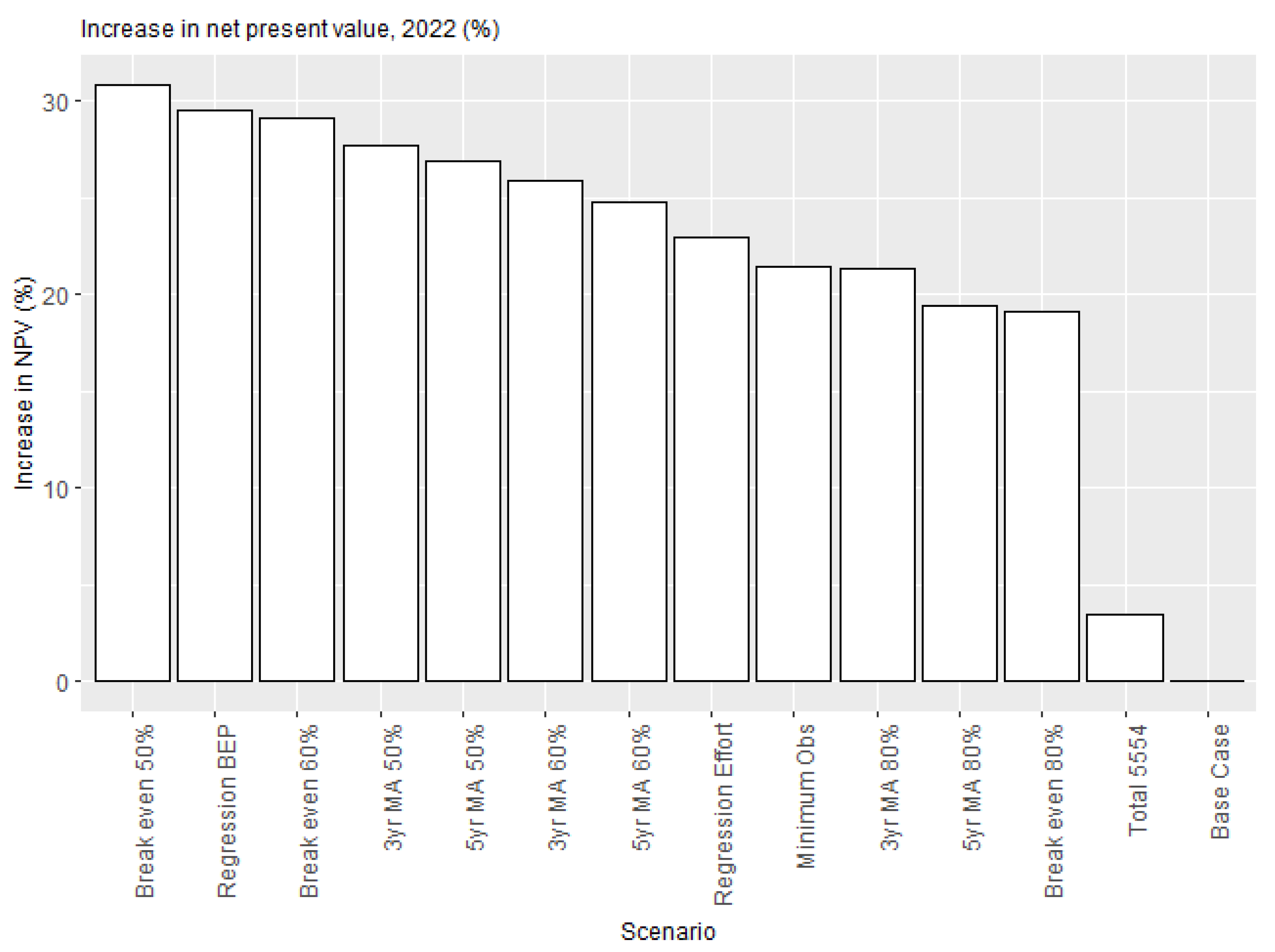
3.3. Bioeconomic Model Results

The potential threshold effort levels (

Table 4. Summary of potential threshold effort levels tested using the bioeconomic model.

	2018	2022
5-year moving average
80%	4316	3951
60%	3237	2963
50%	2698	2469
3-year moving average
80%	4241	3612
60%	3181	2709
50%	2651	2258
Breakeven probability
80%	4000	4000
60%	1800	1800
50%	1200	1200
Regression models
Breakeven point model	1670	1670
Nominal Effort model	3305	3305
Minimum observed	3599	3599

) were applied to the NPF bioeconomic model. Two variants of the model were used—one based on stock and economic conditions in 2018 and the other based on conditions in 2022.

The minimum effort constraint had no substantial impact on the results from the 2018 model, except for the baseline effort constraint (2777 days on each species’ métier), which forced additional fishing effort onto brown tiger prawns in particular (Figure 6). The blue line in Figure 6 represents the observed fishing effort allocated to each of the two tiger prawn species’ métiers. Except for the current baseline constraint, effort on the brown tiger prawn métier was slightly underestimated, while that on the grooved tiger métier was slightly overestimated. The combined effort across both métiers was similar in all cases and close to the observed level of fishing effort in 2018 (Figure 6). The net present value of profits over time was also almost identical between the different minimum effort constraints.

In 2022, the fishery conditions were substantially different to those in 2018. Tiger prawn stocks were estimated to be relatively low and fuel prices high [28]. As noted above, the model results were not adopted as the TAE for 2022 as the high base case threshold (2777 days each métier) resulted in recommended effort levels higher than observed in 2021 despite the adverse stock status and economic conditions. With the exception of the base case and 5554-day overall scenarios, the model-estimated fishing effort for 2022 with the alternative threshold values was similar to the observed fishing effort at the fishery level, but underestimated the effort applied to the grooved tiger métier and overestimated the effort in the brown tiger métier relative to what was observed (Figure 7). Given the observed level of fishing effort was constrained by an ad hoc reduction (rather than based on maximizing net economic returns over time) [22], some difference in the outcomes would be expected. In most cases, the difference between the observed and model-estimated effort values were less than around +/−20% (Figure 8).

Changes in the net present value of fishery profits varied substantially, with most alternative scenarios resulting in between 20–30% higher values than the base case (Figure 9). However, there is a clear trade-off between effort reduction and NPV, with the greatest increases in NPV being a result of the greatest decrease in fishing effort (as might be expected) (Figure 10). Given that there are additional costs associated with reducing fishing effort that are not captured in the model [7], an appropriate minimum effort level to apply in the model may be considered to be within +/−10% of the observed level. Four scenarios fall within this range—three of which are based on a moving average and the fourth based on the regression analysis of the observed fishing effort over time (Figure 10).

4. Discussion and Conclusions

The use of a minimum constraint on fishing effort in dynamic bioeconomic models has the dual role of preventing “bang-bang” solutions while also recognizing the potential social and indirect economic benefits associated with maintaining a level of fishing effort each year. While the principle is well recognized, determining the appropriate value to impose in the models is less straightforward and, to date, has largely been ad hoc.

In this study, a range of different approaches to deriving an appropriate threshold effort level when using such a dynamic bioeconomic model were developed and evaluated. Of the options that were evaluated, the approaches that produced the lowest effort threshold also resulted in the highest net present value of fishery profits. This is not unexpected, as this also allows the fastest stock recovery and subsequently higher future profitability levels.

Given that fishers are, individually, profit maximisers, and hence would only fish provided the marginal benefit (i.e., the value of their catch) exceeded their margin cost given the prevailing stock status and economic conditions, comparing the estimated threshold values to the observed level of effort in 2022 provides another estimate of the breakeven conditions in 2022 based on observed behaviour under adverse biological and economic conditions. Minimum effort thresholds above this value are unlikely to be economically viable (at least in 2022), otherwise fishers (who were unconstrained) would have operated at these higher levels. For this reason, we focused on threshold values that were close to the observed level of fishing effort in 2022.

Of the methods most consistent with the observed level of effort (+/−10%), three of these involved the use of a moving average. An advantage of the moving average approach, other than its pragmatism, is that it also captures the effects of recent conditions in the fishery. This provides a dynamic threshold rather than a static value applied in all conditions, a pertinent consideration when modelling highly variable stock, such as prawns. As the minimum should, by definition, be more conservative than the observed (rather than forcing a higher level of fishing effort than might “naturally” occur given the conditions), the two measures that are potentially most appropriate were 60% of the 3-year moving average or 50% of the 5-year moving average. Both of these measures result in a lower NPV than more conservative values, but capture some of the other benefits by maintaining fishing effort in the fishery.

The use of a moving-average based approach also has some limitations, as it provides less certainty about the future operating environment in the fishery and may, in some cases, overly constrain or under-constrain the fishery if effort levels fluctuate substantially. For example, a rapid decline in stock levels may lead to actual fishing effort falling faster than the moving average, such that the model constraint cannot adjust appropriately. Conversely, rapid recovery, as may be the case in short-term species such as prawns, may result in the minimum constraint being too low, limiting the activity of the fleet unnecessarily. While a fixed value may also lead to under- or over-constraining the model, this provides greater certainty as to minimum allowable effort levels in the fishery to ensure that crew are appropriately retained and markets secured.

The aim of this study was to identify potential minimum effort levels to apply in a dynamic model for use in setting total allowable effort levels. Previously, as in many other cases (e.g., [11]), these were based on what was considered an acceptable minimum level of effort by industry [20]. This, however, resulted in a minimum effort level being imposed in the model that was over 90% of the maximum effort observed in the fishery since 2007. This ad hoc approach and resulting high minimum effort level was found to be problematic when conditions in the fishery became adverse.

Of the options considered in this analysis, the pragmatic use of a moving average, and an appropriate proportion of this (i.e., 50–60%) allows for changes in fishery conditions to be considered in the model while still maintaining a degree of stability. Although, as noted above, the use of moving averages also bring other challenges. Breakeven approaches, while appealing, were found to result in substantially lower levels of fishing effort but higher net present values of profits as measured in the model. As not all benefits of maintaining a minimum level of fishing effort are captured in the model [7], the breakeven approaches may be too conservative.

The direct applicability of the results of this analysis to other fisheries is likely to be limited as each fishery will have its own unique economic, social and ecological conditions. However, the general principles established in this study are likely to be more broadly applicable. These include the justification for considering a minimum effort level when using models to estimate fishing effort or catch limits, and the use of a proportion of moving averages as this minimum is likely to allow some dynamism in the analysis, reflecting the more recent conditions in the fishery. While more complex approaches are also possible (such as the breakeven and regression-based approaches applied in this study), the additional complexity may not be warranted. Nevertheless, also considering these approaches does provide a broader information set upon which final decisions as to which approaches to adopt for the fishery can be based.

References

1. Stephenson, R.L.; Wiber, M.; Paul, S.; Angel, E.; Benson, A.; Charles, A.; Chouinard, O.; Edwards, D.; Foley, P.; Lane, D.; et al. Integrating diverse objectives for sustainable fisheries in Canada. Can. J. Fish. Aquat. Sci. 2019, 76, 480–496. [Google Scholar] [CrossRef]
2. Hornborg, S.; van Putten, I.; Novaglio, C.; Fulton, E.A.; Blanchard, J.L.; Plagányi, É.; Bulman, C.; Sainsbury, K. Ecosystem-based fisheries management requires broader performance indicators for the human dimension. Mar. Policy 2019, 108, 103639. [Google Scholar] [CrossRef]
3. Thébaud, O.; Nielsen, J.R.; Motova, A.; Curtis, H.; Bastardie, F.; Blomqvist, G.E.; Daurès, F.; Goti, L.; Holzer, J.; Innes, J.; et al. Integrating economics into fisheries science and advice: Progress, needs, and future opportunities. ICES J. Mar. Sci. 2023, 80, 647–663. [Google Scholar] [CrossRef]
4. Clark, C. Mathematical Bioeconomics; John Wiley & Sons: New York, NY, USA, 1976. [Google Scholar]
5. Andersen, P.; Sutinen, J.G. Stochastic Bioeconomics: A Review of Basic Methods and Results. Mar. Resour. Econ. 1984, 1, 117–136. [Google Scholar] [CrossRef]
6. Steinshamn, S.I. A Conceptional Analysis of Dynamics and Production in Bioeconomic Models. Am. J. Agric. Econ. 2011, 93, 803–812. [Google Scholar] [CrossRef]
7. Larkin, S.L.; Alvarez, S.; Sylvia, G.; Harte, M. Practical Considerations in Using Bioeconomic Modelling for Rebuilding Fisheries; OECD Food, Agriculture and Fisheries Papers, No. 38; OECD Publishing: Paris, France, 2011. [Google Scholar]
8. Merino, G.; Maynou, F.; García-Olivares, A. Effort dynamics in a fisheries bioeconomic model: A vessel level approach through Game Theory. Sci. Mar. 2007, 71, 537–550. [Google Scholar] [CrossRef]
9. Bartelings, H.; Hamon, K.G.; Berkenhagen, J.; Buisman, F.C. Bio-economic modelling for marine spatial planning application in North Sea shrimp and flatfish fisheries. Environ. Model. Softw. 2015, 74, 156–172. [Google Scholar] [CrossRef]
10. Punt, A.E.; Deng, R.A.; Dichmont, C.M.; Kompas, T.; Venables, W.N.; Zhou, S.; Pascoe, S.; Hutton, T.; Kenyon, R.; van der Velde, T.; et al. Integrating size-structured assessment and bioeconomic management advice in Australia’s northern prawn fishery. ICES J. Mar. Sci. 2010, 67, 1785–1801. [Google Scholar] [CrossRef]
11. Vergara-Solana, F.J.; Vargas-López, V.G.; Bolaños-Durán, E.; Paz-García, D.A.; Almendarez-Hernández, L.C. Bioeconomic analysis of stock rebuilding strategies for the green abalone fishery in Mexico under climate uncertainty. Ocean Coast. Manag. 2023, 243, 106759. [Google Scholar] [CrossRef]
12. Bhat, M.G.; Bhatta, R. Mechanization and technical interactions in multi-species Indian fisheries: Implications for economic and biological sustainability. Mar. Policy 2006, 30, 237–248. [Google Scholar] [CrossRef]
13. Jardim, E.; Urtizberea, A.; Motova, A.; Osio, C.; Ulrich, C.; Millar, C.; Mosqueira, I.; Poos, J.J.; Virtanen, J.; Hamon, K.J.J.S. Bioeconomic Modelling Applied to Fisheries with R/FLR/FLBEIA; JRC Scientific Policy Report EUR 25823 EN; Joint Research Centre: Ispra, Italy, 2013. [Google Scholar]
14. Hoff, A.; Frost, H. Modelling combined harvest and effort regulations: The case of the Dutch beam trawl fishery for plaice and sole in the North Sea. ICES J. Mar. Sci. 2008, 65, 822–831. [Google Scholar] [CrossRef]
15. Péreau, J.C.; Doyen, L.; Little, L.R.; Thébaud, O. The triple bottom line: Meeting ecological, economic and social goals with individual transferable quotas. J. Environ. Econ. Manag. 2012, 63, 419–434. [Google Scholar] [CrossRef]
16. Martinet, V.; Thébaud, O.; Doyen, L. Defining viable recovery paths toward sustainable fisheries. Ecol. Econ. 2007, 64, 411–422. [Google Scholar] [CrossRef]
17. Gourguet, S.; Macher, C.; Doyen, L.; Thébaud, O.; Bertignac, M.; Guyader, O. Managing mixed fisheries for bio-economic viability. Fish. Res. 2013, 140, 46–62. [Google Scholar] [CrossRef]
18. Cissé, A.A.; Gourguet, S.; Doyen, L.; Blanchard, F.; Péreau, J.C. A bio-economic model for the ecosystem-based management of the coastal fishery in French Guiana. Environ. Dev. Econ. 2013, 18, 245–269. [Google Scholar] [CrossRef]
19. AFMA. Northern Prawn Fishery Harvest Strategy 2022; Australian Fisheries Management Authority: Canberra, Australia, 2022. [Google Scholar]
20. Australian Fisheries Management Authority. Northern Prawn Fishery Resource Assessment Group (NPRAG) Meeting Minutes, May 2008; Australian Fisheries Management Authority: Canberra, Australia, 2008. [Google Scholar]
21. Dichmont, C.M.; Jarrett, A.; Hill, F.; Brown, M. Harvest Strategy for the Northern Prawn Fishery under Input Controls; Report to the Australian Fisheries Management Authority, Project 2006/828; CSIRO: Brisbane, Australia, 2012. [Google Scholar]
22. Australian Fisheries Management Authority. Northern Prawn Fishery Resource Assessment Group (NPRAG) Meeting Minutes, 17–18 May 2022; Australian Fisheries Management Authority: Canberra, Australia, 2022. [Google Scholar]
23. Vance, D.J.; Rothlisberg, P.C. Chapter One—The biology and ecology of the banana prawns: Penaeus merguiensis de Man and P. indicus H. Milne Edwards. Adv. Mar. Biol. 2020, 86, 1–139. [Google Scholar] [PubMed]
24. Vance, D.J.; Staples, D.J.; Kerr, J.D. Factors affecting year-to-year variation in the catch of banana prawns (Penaeus merguiensis) in the Gulf of Carpentaria, Australia. ICES J. Mar. Sci. 1985, 42, 83–97. [Google Scholar] [CrossRef]
25. Zeileis, A.; Kleiber, C.; Jackman, S. Regression Models for Count Data in R. J. Stat. Softw. 2008, 27, 1–25. [Google Scholar] [CrossRef]
26. R Core Team. R: A Language and Environment for Statistical Computing; R Foundation for Statistical Computing: Vienna, Austria, 2023. [Google Scholar]
27. Meteyard, B. Northern Prawn Fishery Data Summary 2022; NPF Industry Pty Ltd., Australian Fisheries Management Authority: Canberra, Australia, 2023. [Google Scholar]
28. Deng, R.A.; Miller, M.; Upston, J.; Hutton, T.; Moeseneder, C.; Punt, E.A.; Pascoe, S. Status of the Northern Prawn Fishery Tiger Prawn Fishery at the End of 2021 with Estimated TAEs for 2022 and 2023; Report to the Australian Fisheries Management Authority, October 2022. AFMA Project No. 2020/0803; Australian Fisheries Management Authority: Canberra, Australia, 2022. [Google Scholar]
Figure 1. Average vessel profit if no fishing for tiger prawns occurred compared with banana prawn fishery revenue.
Sustainability 15 16933 g001
Figure 2. Number of days fishing for tiger prawns required to break even.
Sustainability 15 16933 g002
Figure 3. Probability of breaking even at different number of days fished. The vertical black dashed line represents the maximum observed number of days fished, and the vertical blue dashed line the current effort constraint.
Sustainability 15 16933 g003
Figure 4. Annual predicted breakeven point and probability of a zero breakeven point for the period 2007 to 2022. The dashed line represents the base level breakeven point.
Sustainability 15 16933 g004
Figure 5. Nominal fishing effort and average net revenue per day in the tiger prawn fishery.
Sustainability 15 16933 g005
Figure 6. A comparison of key results between the different minimum effort threshold methods applied to the 2018 bioeconomic model and the observed fishing effort in 2018 (the blue line).
Sustainability 15 16933 g006
Figure 7. A comparison of key results between the different minimum effort threshold methods applied to the 2022 bioeconomic model and the observed fishing effort in 2022 (the blue line).
Sustainability 15 16933 g007
Figure 8. Difference between model estimated and observed effort, 2022.
Sustainability 15 16933 g008
Figure 9. Increase in NPV with different effort thresholds relative to the base case.
Sustainability 15 16933 g009
Figure 10. Trade-off between fishing effort and net present value. The blue vertical lines indicate a 10% change from the 2022 observed effort.
Sustainability 15 16933 g010