Study on Spatial Characteristics, Health Assessment, and Influencing Factors of Tropospheric Ozone Pollution in Qin–Jin Region, 2013–2022

Abstract

Ozone is a pollutant that is harmful to human health and the troposphere. As a coal base in China, the study of ozone in the Qin–Jin region provides a scientific basis for pollution control and early warning and is of great practical significance. This paper analyzes the spatial and temporal distribution characteristics of tropospheric ozone in the Qin–Jin region from 2013 to 2022. It predicts the tropospheric ozone seasons in 2023 using a combination of ozone monitoring instruments (OMIs), ground stations, and machine learning. It also estimates the loss of health and economic benefits caused by ozone to humans, discusses the multiple factors affecting ozone changes, and identifies ozone-sensitive pollution control areas. The results showed that ozone in the Qin–Jin region spatially tends to increase from northwest to southeast, the Slope showed that ozone in the study area has a slightly increasing trend (0~0.079), the ozone concentration values are much larger than those in other months during the period of April–September, and there is no weekend effect. The predicted mean ozone values for 2023 are 36.57 DU in spring, 50.88 DU in summer, 34.29 DU in fall, and 30.10 DU in winter. The average values of all-cause mortality and economic losses are estimated to be 4591 and 4214 persons and 43.30 and 51.30 billion yuan in 2019 and 2021 in Shanxi Province, and 2498 and 1535 persons and 23.50 and 18.70 billion yuan in 2019 and 2021 in Shaanxi Province, respectively. Natural factors are positively correlated with ozone in the following order, temperature (TEM) > precipitable water (TPW) > vegetation cover (NDVI) > relative humidity (RH), uplift index (LI) is negatively correlated with ozone, and barometric pressure (PS) is mainly uncorrelated. During the period of high ozone pollution in the Qin–Jin region (April–September), emissions of VOCs accelerated ozone production, and emissions of NOx suppressed ozone production in most areas. The high-value pollution period in the Qin–Jin area is mainly a VOC control area, and the synergistic control of NOx and VOCs is secondary.

1. Introduction

Tropospheric ozone is crucial in the chemical and climatic oxidation of relevant trace gases. Ozone is generated via photochemical reactions involving volatile organic compounds (VOC_S) and nitrogen oxides (NO_X) [1]. High ozone concentrations adversely affect human health [2], forests, and crops [3]. According to the Global Burden of Disease risk reports and epidemiological studies, it is estimated that there were 230,000 deaths worldwide attributable to ozone exposure in 2016 alone [4]. Since promulgating the Clean Air Action Plan in 2013, PM_2.5 emissions have been effectively controlled in all regions, but with our increasing urbanization and economization, the increase in emissions of O₃ precursors (NO_X and VOC_S) in many cities has led to a significant increase in ozone concentrations in most cities in China, with O₃ gradually replacing particulate matter as the primary pollutant in the atmosphere [5]. Being able to timely and accurately grasp the spatial and temporal distribution of high-altitude and ground-level O₃ and its evolutionary characteristics at large scales can effectively solve the O₃ pollution problem and improve air quality, which is a crucial task for current and future research and actions in the field of global academia and atmospheric governance.

Most previous scholars have centered their research around the near-surface O₃ problem. Lu et al. observed that China had more than 29 days with daily average maximum 8 h ozone concentrations exceeding 150 µg/m³ from 2013 to 2017, which is higher than most other regions worldwide [6]. Dai et al. indicated an increase of 36 µg/m³ (49.50%) in annual mean maximum 8 h ozone in the Yangtze River Delta from 2014 to 2019 [7]. When analyzing the intercontinental sources of surface ozone in Europe, Ren et al. found that intercontinental ozone from the tropics contributes about 8.580 µg/m³ to European surface ozone, while more comes from long-range ozone transport from mid-latitudes [8]. Regional and long-term ozone pollution events are occurring more frequently in China [9]. In contrast, there are very few detections, analyses, and simulations of the characteristics of the spatial and temporal distribution of O₃ concentration and its evolution within the entire atmospheric column or troposphere. With the development of space remote sensing technology, satellite remote sensing provides the possibility of obtaining global or regional-scale detection data, and the essential feature of satellite remote sensing detection technology, compared with ground-based monitoring, lies in the fact that it can realize all-weather, high-temporal- and -spatial-resolution, and higher-precision continuous observation of O₃ over a wide range of areas on a global scale. However, there are multiple errors in the ozone data source due to the interference of influences such as radiation, parameters, and cloud cover during the use of satellite data. The OMI satellite remote sensing used in this study has better spatial resolution compared to the Global Ozone Monitoring Experiment (GOME) and the Scanning Imaging Absorption Spectrometer for Atmospheric Mapping (SCHIMACHY), allowing it to characterize atmospheric chemistry from space better [10]. In conclusion, studying the temporal and spatial dynamic characteristics of O₃ concentration at high altitudes and its evolution trend based on satellite data is a hot spot of atmospheric environment research.

Many studies have shown that anthropogenic emissions are the main driver of the increase in surface ozone in different regions of China and different years. However, at the same time, the influence of meteorological parameters may also be significant. Li et al. indicate that anthropogenic emissions are the leading cause of the increase in surface ozone in China from 2013 to 2019 [11]. Liu and Wang concluded that anthropogenic factors dominate most of the ozone changes in China, but the influence of meteorological conditions may be more significant in some areas [12]. Gong et al. found that about 57–80% of the increase in ground-level ozone from 2013 to 2020 in Chinese cities could be due to meteorological causes [13]. Many studies have reduced ozone concentrations by controlling ozone precursors, as well as activities such as reducing anthropogenic emissions of nitrogen oxides. Ozone production shows a highly nonlinear relationship with its precursors (NO_x and VOC_s) [14], and the sensitivity of ozone production can be reflected by the relative amount of VOC_s to NO_x [10]. Ozone trends have received increasing attention since using satellite remote sensing, ground-based observations, and numerical modeling in China.

The Qin–Jin region is located in the central part of China, roughly between 106° E~115° E and 32° N~41° N, with a land area of about 361,900 km², and its administrative area includes Shanxi and Shaanxi provinces (Figure 1). The region’s terrain is high in the north and south and low in the center (Guanzhong Plain), and vegetation is mainly found in the higher mountains. The climate type of the study area mainly belongs to the monsoon climate zone, the temperature difference between day and night is significant, the average annual precipitation ranges from 358 to 931 mm, precipitation is concentrated in the summer and fall seasons, and the precipitation decreases gradually from south to north [15]. The Qin–Jin region is one of the most developed regions in China in terms of mineral resources, and its coal is marketed all over the country [16]. Environmental pressures from the complex terrain and economic growth have led to more severe air pollution problems in the Qin–Jin region.

In recent years, ozone research has been mainly concentrated in the more economically developed areas, while more research needs to be conducted on the changes in the characteristics of O₃ pollution outside the critical prevention and control areas. The overall characteristics of O₃ pollution changes in China, identification of the causes of increased O₃ pollution, and health losses due to ozone pollution have yet to be revealed. Therefore, this paper provides a specific scientific basis for the governance and early warning of ozone pollution in the region and, at the same time, provides an important practical significance for the in-depth evaluation of the rationality and scientificity of the existing pollution joint prevention and control policies. This study aims to characterize the spatial and temporal distribution of tropospheric ozone in the Qin–Jin region from 2013 to 2022 and the prediction of the tropospheric ozone seasons in 2023 by using a combination of remote sensing monitoring by OMI satellites, ground-based stations, and machine learning. Then, the numbers of premature deaths and economic losses due to ozone pollution and population exposure in the study area were calculated and evaluated based on the Benmap model to provide a specific reference basis for China’s ecological and environmental joint health departments to formulate regional air pollution control measures in a targeted manner, as well as for decision making on disease prevention and control and other aspects. And the effects of anthropogenic factors, natural factors, and precursors of pollution on ozone were analyzed. Finally, the localized ozone sensitivity (FNR) was used to perform control analysis for periods of high levels of ozone pollution. This study has great scientific value and practical significance.

2. Data Sources and Methods

2.1. Data Sources

The daily remote sensing data of tropospheric ozone (O₃), nitrogen dioxide (NO₂), and formaldehyde (HCHO) come from the Ozone Monitoring Instrument (OMI), which was launched by the National Aeronautics and Space Administration (NASA) and mounted on the Aura satellite, with a spatial resolution of 0.25° × 0.25°. Ground-level ozone (O₃) hourly concentration data were provided by the National Urban Air Quality Real-time Distribution Platform of the China Environmental Monitoring General Station (http://www.mee.gov.cn/, accessed on 1 June 2023), and 109 stations were covered in this study, with the daily maximum 8 h average ozone concentration (MDA8-O₃, µg/m³) considered to be the daily ozone level in the city. This paper uses remote sensing monitoring data of pollutants to map the spatial and temporal distribution of tropospheric column ozone concentrations in the study area, and station monitoring data were used to assess surface ozone concentrations and health economic losses due to population exposure.

Precipitable precipitation (SVP), temperature (TEM), pressure (PS), lift index (LI), and relative humidity (RH) data were obtained from the NOAA Weather Monitoring Network (https://psl.noaa.gov/data/gridded/data.ncep.reanalysis.surface.html, accessed on 1 June 2023) of the U.S. NCEP-NCAR Global Atmospheric Reanalysis dataset. Normalized difference vegetation index (NDVI) and population density (POP) data were obtained from the Resource Science Data Center of the Chinese Academy of Sciences. In this study, ozone remote sensing monitoring data were utilized to conduct correlation and kernel density analyses with influencing factors, aiming to examine the varying degrees of influence on ozone.

The land use data were obtained from the annual China Land Cover Dataset (CLCD) produced by Prof. Yang Jie and Prof. Huang Xin from Wuhan University based on 335,709 Landsat images on Google Earth Engine. The present study employed land use and elevation data to generate a comprehensive cartographic representation of the research area.

2.2. Research Methods

2.2.1. Analysis of Past (Slope) and Future (Random Forest Machine Learning) Trends

In order to investigate the interannual spatial and temporal variations in tropospheric ozone column concentrations in the Qin–Jin region during the period 2013–2022, this study employed David Freedman’s univariate linear regression analysis in statistics to characterize the spatiotemporal dynamics of regional tropospheric ozone column concentrations over the past decade. The absolute value of ${\theta }_{slope}$ indicates the magnitude of the trend, and the larger the absolute value, the more pronounced the change, with positive values showing an increasing trend and negative values showing a decreasing trend. The graphs were analyzed using Python 3.6. The advantage is the visualization and simulation of the evolution of the regional pattern of different image elements at different times.

Random forest is a machine learning method based on classification trees. In 1984, Breiman et al. introduced the classification and regression tree [17], while in 2001, Breiman incorporated Ho’s method from Bell Labs [18]. The advantage of this method is that it increases the prediction accuracy without a significant increase in computation. Random forest machine learning is based on the principle of repeated sampling of the set of input training samples with N put-backs using the bootstrap method, using the criterion of tree passing down the tree and out-of-bag data to review the model, and the split will be stopped if the mean square error is too large. Generating a forest tree requires setting three primary parameters: decision estimations, maximum depth of models, and random state numbers. This study utilized Python GDAL, Pandas, Numpy, Scipy, Sklearn, and Jupyter modules for data reading, raster computation, and image generation.

2.2.2. Benmap-Model-Based Health Impact Function and Economic Loss Assessment

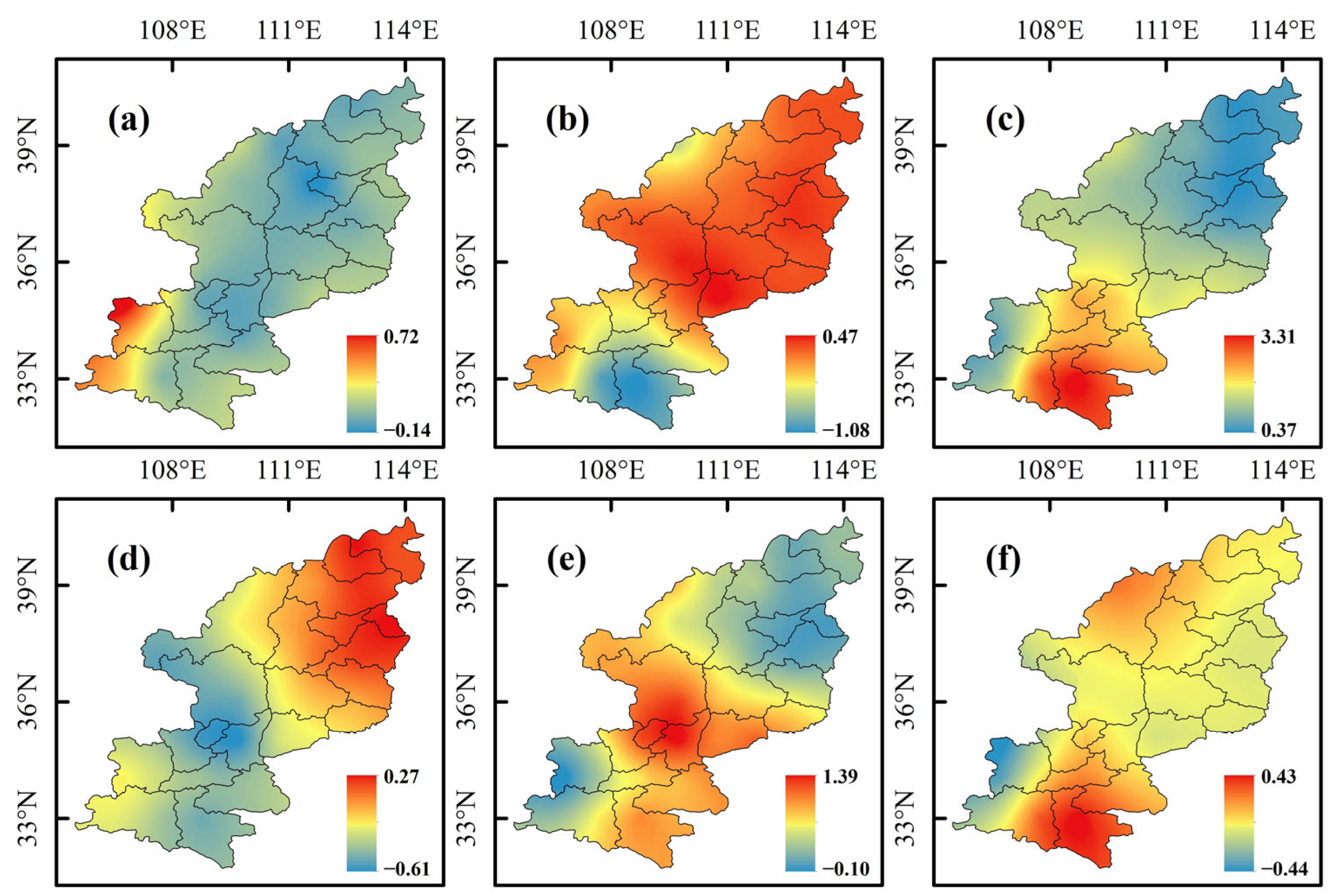
The health effect endpoints selected for this study were all-cause mortality, cardiovascular mortality, and respiratory mortality. Their corresponding International Classification of Diseases codes (ICD10) were A00-R99, I00-I99, and J00-J98. Baseline mortality data were obtained from the 2020 to 2022 China Health and Wellness Statistical Yearbook. Exposed population data were sourced from the Shanxi Provincial Statistical Yearbook and the year-end resident population from the Shaanxi Provincial Statistical Yearbook. GDP per capita and consumer price index were retrieved from previous National Statistical Yearbooks, while purchasing power parity index was obtained from the World Bank’s PPP conversion factor database. The advantages of the Benmap-based model are reduced data computation, improved accuracy of the results, and the ability to visualize the results. The concentration threshold ozone MDA8 was determined as 57.24 µg/m³ based on Turner et al.’s research [19], with specific exposure–response factors detailed in

Table 1. Exposure–response coefficient of health effects.

Health Effect Terminal	β (%)	95%CI (%)
All-cause mortality [20]	0.024	0.013–0.035
Cardiovascular mortality [20]	0.027	0.010–0.044
Respiratory mortality [21]	0.073	0.049–0.097

Note: β represents the proportional increase in mortality risk within the population associated with each 1 µg/m³ increment in O₃ concentration.

.

In order to quantitatively characterize the impact of ozone pollution on population health, an estimation was made for the number of premature deaths resulting from illnesses caused by ozone pollution. This was achieved through the construction of a health effect function incorporating concentration–response coefficients, which were calculated as follows:

$$\Delta Y=\left(1-e^{-\beta \Delta X}\right)\times Incidence\times POP$$

(1)

$$\Delta X=\frac{\Delta X_{out}}{\Delta X_{exposure}}$$

(2)

where $\Delta Y$ is the valuation of the health effect of ozone pollution, $\Delta X$ is the change in ozone concentration, $\beta$ is the concentration–response coefficient, $Incidence$ is the baseline incidence of the endpoints of the health effect, $POP$ characterizes the number of exposed populations, $\Delta X_{out}$ is the change in ozone concentration, and $\Delta X_{exposure}$ is the exposure factor of ozone concentration.

The willingness-to-pay method was employed in this study to evaluate the variations in surface ozone concentrations, explicitly focusing on changes in the number of healthy terminal deaths. The assessment was conducted using the following formula:

$$VS{L}_{china,year}=VS{L}_{china,year0}\times {\left(\frac{Y_{china,year}}{Y_{china,year0}}\right)}^{\epsilon }\times PP{P}_{year0}\times \frac{CP{I}_{china,year}}{CP{I}_{china,year0}}$$

(3)

where $VS{L}_{china,year}$ is the value of vital statistics in the target year (RMB), $VS{L}_{china,year0}$ is the value of vital statistics in the base year (USD), Y is the GDP per capita (USD), PPP is the purchasing power parity index (unit: RMB/USD), CPI is the consumer price index, and $\epsilon$ is the elasticity coefficient, which is usually taken as 0.8. In this paper, we take the value of life statistics of domestic residents in 2011 (828,068 USD) as the base value and obtain the final economic benefits result (E) through Equations (2)–(4), which are calculated as follows:

$$E=\Delta Y\times VS{L}_{china,year}$$

(4)

2.2.3. GTWR

Geographically and Temporally Weighted Regression (GTWR) is a spatial geographically weighted regression model, developed by Huang et al. (2010), which incorporates temporal characteristics into the model composition. It expresses the quantitative dependence of variables through regression equations, enabling a comprehensive reflection of the influence of spatial location characteristics and temporal factors in the model [22]. The GTWR model is a local linear regression model that simultaneously incorporates spatiotemporal non-stationarity, capturing the relationship between a series of observations (Y₁, Y₂, …, Y_i) at the spatial location (u_i, v_i) and time t_i, and the dependent variables x_i1, x_i2, …, x_ik. This relationship can be expressed as follows:

$$y_i={\beta }_0\left({\mu }_{\mathrm{i}},v_i,t_i\right)+{{\displaystyle \sum }}_{k=1}^P{\beta }_k\left({\mu }_{\mathrm{i}},v_i,t_i\right)x_{ik}+{\epsilon }_i\left(\mathrm{i}=1,2,3\dots n\right)$$

(5)

where $\mathrm{i}=1,2,\dots ,\mathrm{k},Y_i$ denotes the predicted urban ozone concentration, ${\beta }_0$ denotes the intercept, $\left({\mu }_{\mathrm{i}},v_i,t_i\right)$ is the spatiotemporal geographic location corresponding to the $\mathrm{i}$ sample point, ${\beta }_{1..k}$ is the regression coefficient of the sample point $\left({\mu }_{\mathrm{i}},v_i,t_i\right)$, and ${\epsilon }_i$ denotes the residuals of the sample points $\left({\mu }_{\mathrm{i}},v_i,t_i\right)$.

2.2.4. Kernel Density Analysis

Kernel density estimation (KDE) is a spatial density analysis method based on a clustering algorithm for data density functions, in which higher weights are assigned to events $x_i$ neighboring the sample centroid. In comparison, events farther away from the centroid $x$ are assigned lower weights [23]. We used points of interest (POIs) to spatially assign non-point-source pollution and spatially visualized POI through kernel density analysis to obtain aggregated characteristics of highly coupled functional entities and human activities. The calculation formula is

$$\int h\left(x\right)=\frac{1}{n{h}^d}{{\displaystyle \sum }}_{i=1}^{n}K\left(\frac{x-x_i}{h}\right)$$

(6)

where $K\left(x-x_i/h\right)$ denotes the kernel function form, usually as a symmetric single-peak probability density function. $h$ is the bandwidth, a free parameter defining the magnitude of the smoothing amount. $d$ is the latitude of the data. $n$ is the number of points of point $i$ within the bandwidth.

2.2.5. Ozone Sensitivity (FNR)

$$FNR=c\left(HCHO\right)/c\left(N{O}_2\right)$$

(7)

where $c\left(HCHO\right)$ is the HCHO column concentration in 10¹⁵ molec/cm² for the grid in the administrative area and $c\left(N{O}_2\right)$ is the NO₂ column concentration in 10¹⁵ molec/cm² for the grid in the administrative area.

The criteria for determining ozone sensitivity in this paper are the criteria FNR < 3.2 for VOC_s control (reduction in VOCs effectively suppresses ozone production), FNR > 4.3 for NO_x control (reduction in NO_x effectively suppresses ozone production), and 3.2 < FNR < 4.3 for NO_x-VOC_s synergistic control (reduction in either NO_x or VOCs effectively suppresses ozone production) [24].

This paper is organized around the ideas in Figure 2 to study and explore.

3. Results and Discussion

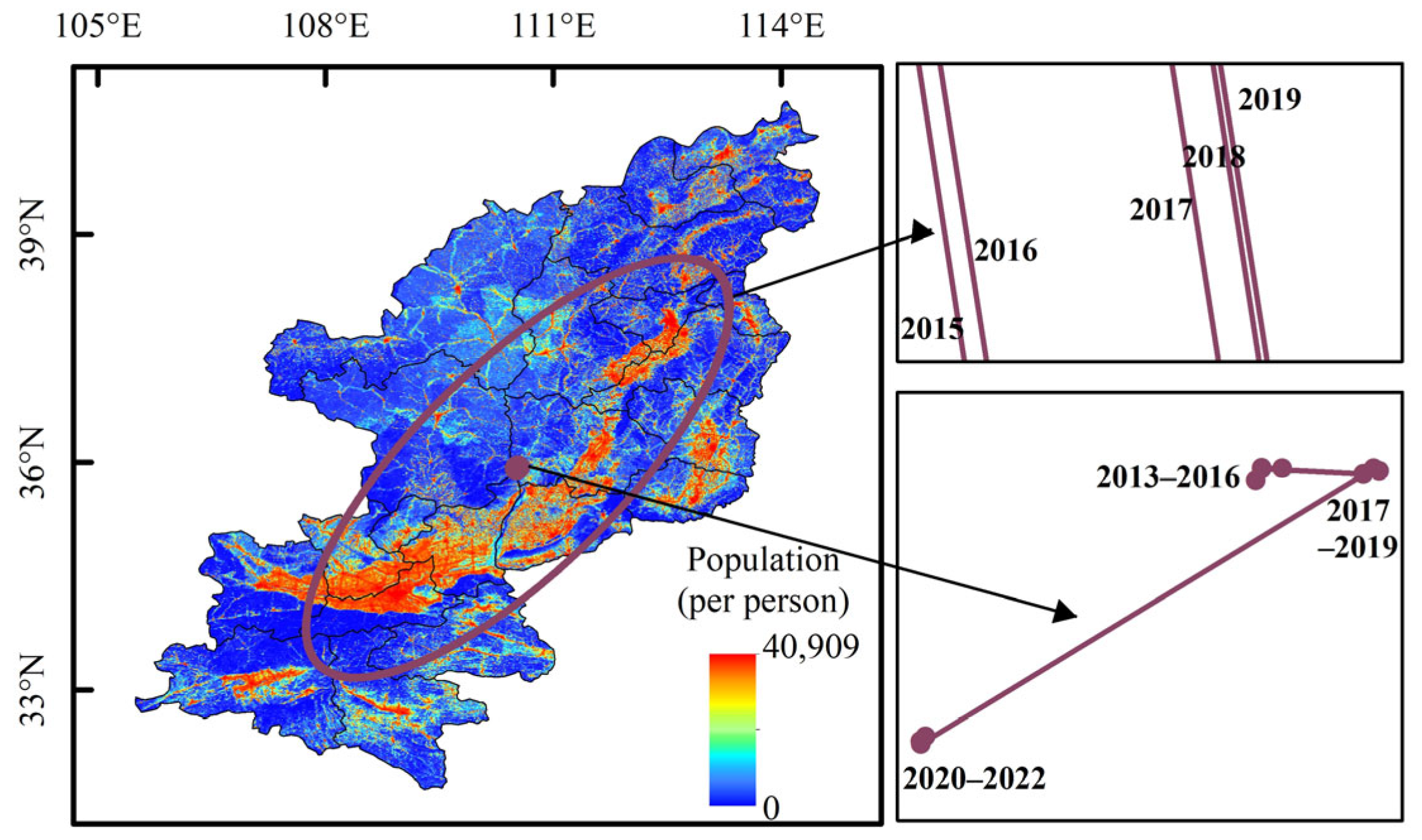
3.1. Temporal–Spatial Distribution and Change Trend of Ozone

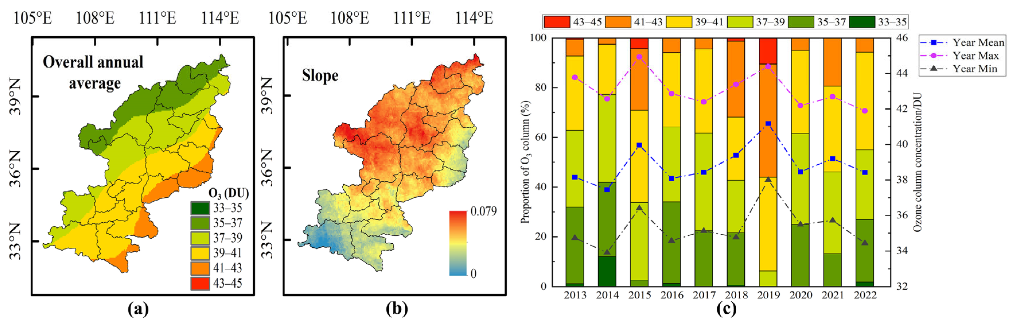
3.1.1. Characterization of the Interannual Distribution of Tropospheric Ozone

In this paper, when processing the data, the strip with storage format HDF is used to extract the tropospheric ozone column concentration day-by-day data with the conditions of latitude, longitude, time, and concentration. In order to ensure accuracy, the boundary range of the extraction of the study area is enlarged by 0.3–0.5°, and the anomalies, innumerable data points, and the points with cloudiness greater than 0.2 are eliminated by utilizing Python 3.9 to enhance the credibility. The raster processing is carried out by using the Kriging interpolation method. Concentration data with an accuracy of 0.01 image elements were finally obtained. The spatial and temporal distribution of the tropospheric ozone column concentration in the Qin–Jin region from 2013 to 2022 are depicted in Figure 3a, revealing an increasing trend of ozone concentration from northwest to southeast. Figure 3b employs Slope analysis to provide a comprehensive understanding of the historical trend of ozone concentration, and all calculated results are statistically significant at the 95% confidence level. They indicate a slight upward trend in tropospheric ozone column concentration across all regions within the study area during the past decade. This trend is particularly prominent in the northern part of the study area, with Datong, Shuozhou, Lvliang (Shanxi Province), and Yulin, Yan’an (Shaanxi Province), experiencing faster ozone growth rates than other regions. The classifications depicted in Figure 3c align with the classification criteria illustrated in Figure 3a, which were derived by quantifying the proportion of tropospheric ozone coverage within distinct categories. Level II (35–37 DU), Level III (37–39 DU), and Level IV (39–41 DU) accounted for 20.26%, 29.20%, and 32.11% of the total, respectively. The tropospheric column ozone concentration in the study area exhibited two significant increases in 2015 and 2019, with the mean ozone concentration (37.45 DU) reaching its lowest point in 2014 and attaining the highest level in a decade (41.18 DU) in 2019.

Compared to other regions, the mean annual tropospheric column ozone concentration in the Qin–Jin region is 38.87 DU, which is lower than the mean tropospheric column ozone concentration near 30° N in Europe, Africa, and East Asia (45 DU) but higher than that in Southeast Asia extending to western America across the Pacific Ocean (15–20 DU). This distribution primarily correlates with the spatial distribution of ozone precursors [25]. In China, urban agglomerations within the Beijing–Tianjin–Hebei region, Yangtze River Delta region, Pearl River Delta region, and Chengdu–Chongqing region exhibit higher tropospheric ozone concentrations than those observed in the Qin–Jin region [26].

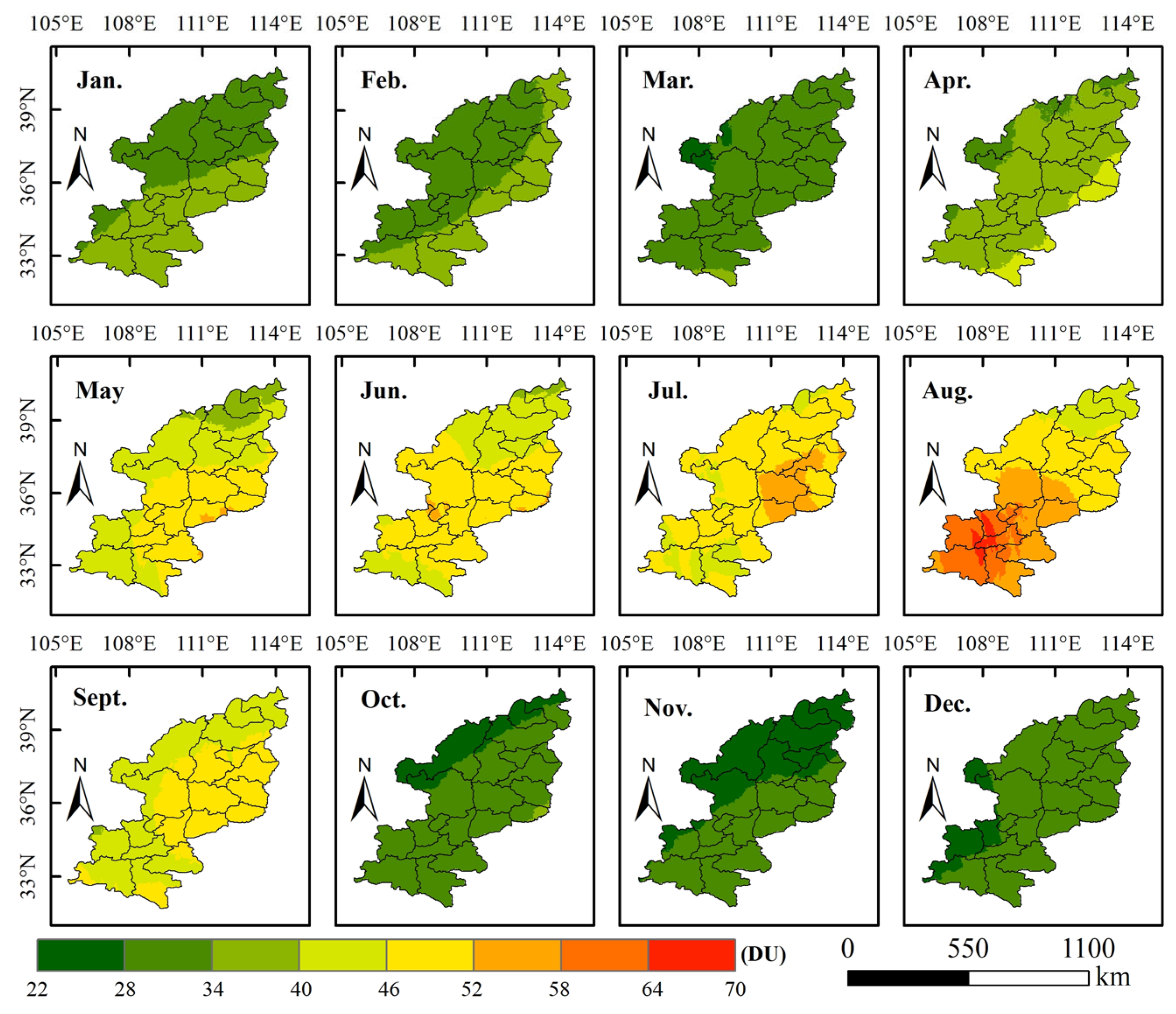
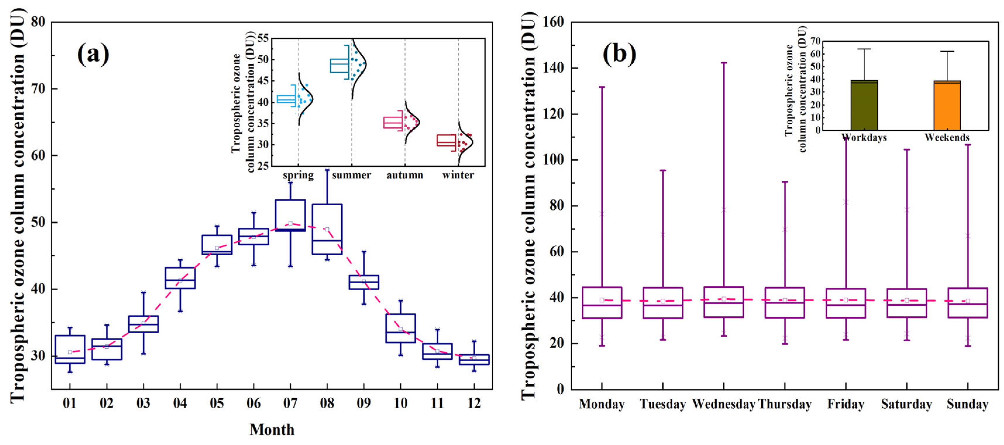
3.1.2. Monthly and Weekly Distribution Characteristics of Tropospheric Ozone

Figure 4 shows the monthly spatial distribution of column ozone concentrations for the Qin–Jin region from 2013 through 2022. For visual analysis, the tropospheric ozone column concentrations were analyzed by the difference between the highest (67.26 DU) and lowest (24.29 DU) values. Based on Figure 3, it is evident that the tropospheric ozone column concentration in the designated study area predominantly exhibits low values within Level I (22–28 DU), Level II (28–34 DU), and Level III (34–40 DU) from January to March. Moreover, there is a gradual decline observed in ozone concentration, with the proportion of the Level III region decreasing from 46.56% in January to merely 1.840% by March, revealing a progressive augmentation in column ozone concentrations within area from April to August. In August, the eighth level (64–70 DU) accounted for 2.910% of the total study area. The monthly average maximum ozone concentration (52.69 DU) was observed in August, and the bordering areas of Xi’an, Xianyang, and Hanzhong were the most polluted during this month. The tropospheric ozone column concentrations in the study area decreased from September to November, with levels III, IV, and V prevailing in September, while levels I and II dominated in October and November, and the proportion of the level II region declined from 79.94% in October to 53.92% in November. The monthly average ozone minimum (28.33 DU) occurred in November. Tropospheric column ozone concentrations in the study area increased slightly in December compared to November and October but remained predominantly primary and secondary. The area of high column ozone concentrations initially emerged in the eastern region of the study area and subsequently expanded progressively towards the west. Overall, ozone concentration values from May to September were higher than the monthly average over the past ten years (38.52 DU), establishing these five months as crucial control periods for ozone pollution within the study area.

The box plots in Figure 5 depict the tropospheric ozone column concentrations in the Qin–Jin region from 2013 to 2022, presenting monthly averages, quarterly averages, and weekly averages. The analysis of concentration dispersion points for each month throughout ten years revealed that the monthly variation in the study area exhibited a unimodal pattern, characterized by peak concentrations exceeding 51.45 DU between April and September, corresponding to months with elevated levels of ozone accumulation. The seasonal variation in ozone levels followed the pattern of summer > spring > fall > winter, with mean ozone values of 37.41DU, 49.47 DU, 34.69 DU, and 32.50 DU observed in the study area during spring, summer, fall, and winter, respectively (Figure 5a). Zhao et al. concluded that the maximum summer ozone gain in China occurs mainly in cities in Shanxi, Henan, and Anhui, which may be related to the progressively higher temperatures and lower summer PM_2.5 levels in these provinces [27]. Cleveland et al. proposed that ozone concentrations during weekends exceeding those on weekdays are referred to as positive weekend effects, while lower concentrations on weekends compared to weekdays are negative weekend effects [28]. The column ozone concentration in the Qin–Jin region showed no significant variation from Monday to Sunday, as depicted in Figure 5b. This study revealed a consistent ozone concentration in the Qin–Jin region between weekdays (Monday through Friday) and rest days (Saturday and Sunday), and average ozone concentrations on weekdays and rest days were 38.99 and 38.73 DU, respectively. This result contradicts the findings of Zhao et al. [29], who reported higher ozone levels on weekends than on weekdays in Beijing. We roughly deduce that motor vehicle emissions and human activities exhibit no significant difference between weekdays and weekends in the Qin–Jin region, where residents’ income levels are comparatively low compared to those of developed cities in China. As a result, weekend leisure activities for local residents are relatively limited when compared to those living in megacities. This trend is closely linked with the growing demand for an improved quality of life.

3.1.3. Characterization of Future Ozone Projections Based on Random Forests

Figure 6 shows the measured ozone values for 2022 and the random forest regression model predictions for four seasons of ozone column concentrations for 2022 and 2023 in the Qin–Jin area. The data source utilized for prediction was the corresponding season’s 108-month ozone concentrations from the previous nine years. In the random forest model, the Gini impurity is generally used as a criterion for passing information down the tree; the smaller the Gini impurity as the tree extends down the tree, the simpler the information. The depth of the tree determines the number of nodes; the more profound the depth, the more accurately the nodes are fitted, but too much depth can lead to overfitting. Models with a number depth of 100, a regression with a minimum value of 5, a categorical value of 1, and a training dataset of 10% were excluded for validation. The final result output R² values ranged from 0.9966 to 0.9992, and the MSE was below 0.0222 for all four transfer assessment scores, all of which performed well. Comparing predicted values with actual values for each season in 2022 revealed similar spatial distribution patterns and ranges of values. So, the random forest regression model constructed in this paper to predict the spatial data of ozone column concentration in the study area for the four seasons in 2023 is reliable.

From the results in Figure 6, it can be seen that the predicted values for spring 2023 (34.15–40.57 DU) and the actual values for spring 2022 (33.23–42.55 DU), the predicted values for summer 2023 (47.64–52.93 DU) and the actual values for summer 2022 (41.42–55.96 DU), the predicted values for fall 2023 (32.14–37.55 DU) and the actual values for fall 2022 (30.57–39.14 DU), and the forecasted values for winter 2023 winter (28.94–30.90 DU) and the actual values for winter 2022 (24.29–33.03 DU) have more different spatial and temporal distributions. Compared to 2022, ozone column concentrations will decrease slightly in spring, fall, and winter in 2023, and the highest values will still be in the southeastern part of the study area. However, ozone column concentrations may be flat or increase slightly in the summer of 2023, and the area of high ozone values will be further expanded, suggesting that increased attention should be paid to the changes in ozone pollution of Qin–Jin in a future summer. The Qin–Jin region has four distinct seasons, a high vegetation cover in the summer, and a positive correlation between HCH and isoprene released from vegetation in the summer, and a high temperature in summer accelerates the efficiency of oxidative and photochemical reactions, which provides prerequisites for accelerating the conversion of VOC_S [30]. During the winter months, the emission of volatile organic compounds (VOC_S) is limited due to plant wilting.

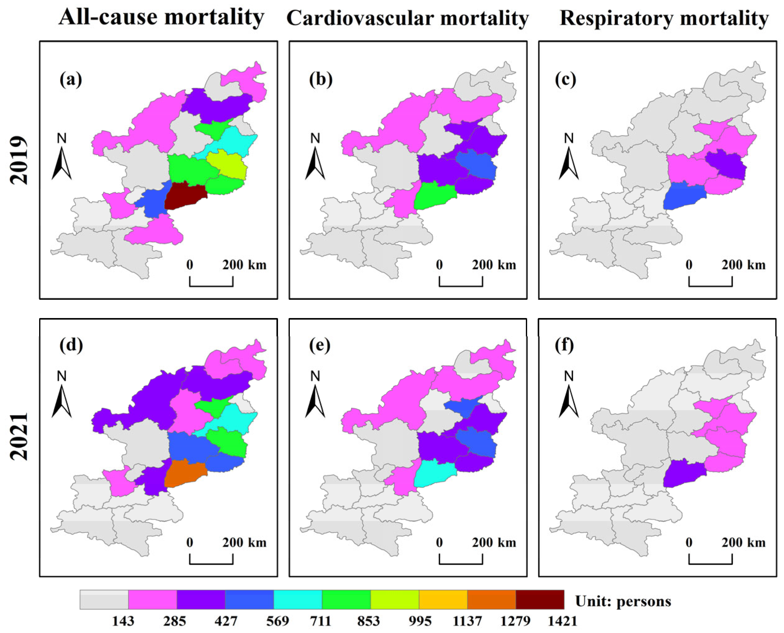
3.2. Number of Premature Deaths from Diseases Associated with Ozone Exposure and Health Economic Assessment

In order to quantify the effects of ozone pollution on human health, the annual average of ozone MDA8 concentrations at influential monitoring stations in the Qin–Jin area was loaded into BenMAP-CE in this study. Firstly, the primary database for health effect assessment was established, encompassing the setup of a spatial grid, the integration of monitoring station data and population spatial data, the selection and configuration of health effect indicators, as well as the development of health impact functions and value measurement functions. Secondly, the spatial distribution of grid-scale ozone concentrations were modeled, and inverse distance weights were computed for the defined spatial grids using the VNA spatial interpolation method [31]. Finally, a model-based assessment was conducted to estimate the magnitude of premature mortality and health economic losses attributed to ozone pollution in the study area. The year 2019 was the year with the highest average ozone concentration in the last decade, and 2021 was the year when the China National Health Commission publicized the earliest year of disease data. Therefore, this paper evaluates the premature deaths and economic losses from three common diseases caused by ozone pollution in 2019 and 2021.

As shown in Figure 7 and

Table 2. The premature mortality rates attributed to ozone pollution in the Qin–Jin region, categorized by city.

Region	All-Cause Mortality (In Persons, 95%CI)		Cardiovascular Mortality (In Persons, 95%CI)		Respiratory Mortality (In Persons, 95%CI)
	2019	2021	2019	2021	2019	2021
Datong	216 (117, 314)	276 (150, 401)	117 (44, 191)	160 (60, 260)	71 (48, 94)	74 (50, 97)
Shuozhou	31 (17, 45)	145 (79, 211)	17 (6, 28)	84 (31, 137)	7 (10, 14)	39 (26, 51)
Xinzhou	393 (214, 570)	358 (195, 520)	214 (80, 345)	208 (78, 337)	87 (128, 168)	95 (65, 125)
Yulin	280 (152, 406)	325 (176, 472)	152 (57, 247)	189 (70, 306)	62 (92, 122)	87 (59, 115)
Yanan	67 (36, 98)	58 (31, 84)	36 (14, 59)	34 (12, 54)	15 (22, 30)	16 (10, 21)
Baoji	86 (46, 125)	100 (54, 146)	47 (17, 76)	58 (22, 95)	28 (19, 38)	27 (18, 36)
Hanzhong	10 (5, 14)	25 (13, 36)	5 (2, 9)	14 (5, 23)	3 (2, 4)	7 (4, 9)
Ankang	11 (6, 17)	51 (27, 74)	6 (2, 10)	30 (11, 48)	4 (2, 5)	14 (9, 18)
Shangzhou	176 (96, 256)	119 (64, 173)	96 (36, 155)	69 (26, 112)	58 (39, 77)	32 (22, 42)
Xi’an	4 (2, 6)	15 (8, 22)	2 (1, 4)	9 (3, 14)	1 (0, 2)	4 (3, 5)
Weinan	480 (261, 697)	329 (179, 479)	261 (97, 423)	192 (71, 311)	106 (158, 208)	88 (60, 117)
Tongchuan	74 (40, 107)	30 (16, 44)	40 (15, 65)	18 (6, 28)	16 (24, 32)	8 (5, 11)
Xianyang	250 (136, 364)	196 (106, 286)	136 (51, 221)	114 (42, 186)	83 (56, 110)	53 (36, 70)
Yuncheng	1421 (779, 2049)	1210 (662, 1747)	772 (291, 1235)	703 (264, 1128)	451 (310, 585)	315 (216, 410)
Jincheng	769 (424, 1101)	558 (305, 806)	416 (159, 660)	324 (122, 520)	237 (166, 304)	145 (100, 189)
Changzhi	953 (522, 1373)	757 (414, 1094)	517 (195, 827)	440 (165, 706)	301 (208, 391)	198 (135, 258)
Linfen	727 (397, 1053)	522 (284, 757)	395 (148, 637)	303 (113, 490)	236 (161, 308)	139 (94, 182)
Taiyuan	774 (422, 1123)	778 (424, 1128)	421 (157, 680)	452 (169, 731)	253 (172, 332)	207 (140, 271)
Lvliang	143 (77, 208)	146 (79, 212)	78 (29, 126)	85 (31, 138)	47 (32, 63)	39 (26, 52)
Yuci	570 (310, 825)	574 (313, 831)	310 (116, 499)	334 (125, 538)	185 (126, 242)	152 (103, 199)
Yangquan	72 (39, 105)	113 (61, 164)	39 (14, 64)	66 (24, 106)	24 (16, 31)	30 (20, 40)

and

Table 3. The health economic losses resulting from ozone of Qin–Jin region, categorized by province.

Region	Year	Disease Name	Number of Premature Deaths (In Persons, 95%CI)	Economic Loss (Hundred Million RMB, 95%CI)
Shanxi	2019	All-cause mortality	4591 (2500, 6659)	433 (236, 628)
		Cardiovascular mortality	2496 (932, 4034)	235 (88, 380)
		Respiratory mortality	1499 (1018, 1969)	141 (96, 186)
	2021	All-cause mortality	4214 (2293, 61,170)	513 (279, 745)
		Cardiovascular mortality	2450 (914, 3965)	298 (111, 483)
		Respiratory mortality	1123 (761, 1478)	137 (93, 180)
Shaanxi	2019	All-cause mortality	2498 (1356, 3634)	235 (128, 342)
		Cardiovascular mortality	1359 (505, 2207)	128 (48, 208)
		Respiratory mortality	826 (557, 1091)	78 (52, 103)
	2021	All-cause mortality	1535 (832, 2235)	187 (101, 272)
		Cardiovascular mortality	893 (332, 1452)	109 (40, 177)
		Respiratory mortality	415 (279, 549)	50 (34, 67)

, the total number of all-cause mortalities in Tongchuan, Yan’an, Xianyang, Xinzhou, Linfen, Jincheng, Changzhi, and Yuncheng increased in 2021 compared to 2019. Additionally, Yuncheng had the highest count of premature deaths due to all causes during both years. However, the premature mortality number due to cardiovascular diseases in Yan’an, Tongchuan, Xianyang, Xinzhou, Linfen, Jincheng, Changzhi, and Yuncheng instead decreased in 2021 compared with 2019, with reduction rates of 5.560%, 55.00%, 16.18%, 2.800%, 23.29%, 22.12%, 14.89%, and 8.940%, respectively. By province, Shanxi Province has more all-cause pre-mortality deaths from ozone pollution than Shaanxi Province. There are more premature deaths from cardiovascular diseases than respiratory diseases in the study area. There was a lower number of premature deaths from ozone pollution in Qin–Jin in 2021 compared to 2019.

The economic losses due to all premature deaths in Shanxi Province were 43.30 and 51.30 billion yuan in 2019 and 2021, and the economic losses due to all premature deaths in Shaanxi Province were 23.50 and 18.70 billion yuan in 2019 and 2021, respectively. Economic losses from ozone pollution were higher in Shanxi Province than in Shaanxi Province, and were elevated in Shanxi Province for both diseases, except for a small decrease in economic health losses from premature mortality from respiratory diseases. The economic health loss from premature death from all three diseases in Shaanxi Province decreased slightly in 2021 compared to 2019.

Increased ozone pollution has put enormous pressure on the increase in disease in China. Ozone pollution in 2017 resulted in approximately 138.1 (95%CI: 52.4, 222.0) disability-adjusted life years (DALYs) lost per 100,000 people and 178,187 (95%CI: 67,650, 286,229) deaths in China [32]. The Chinese scientific community and government agencies are intensifying their focus on ozone pollution due to its significant impact on public health.

3.3. Influencing Factors

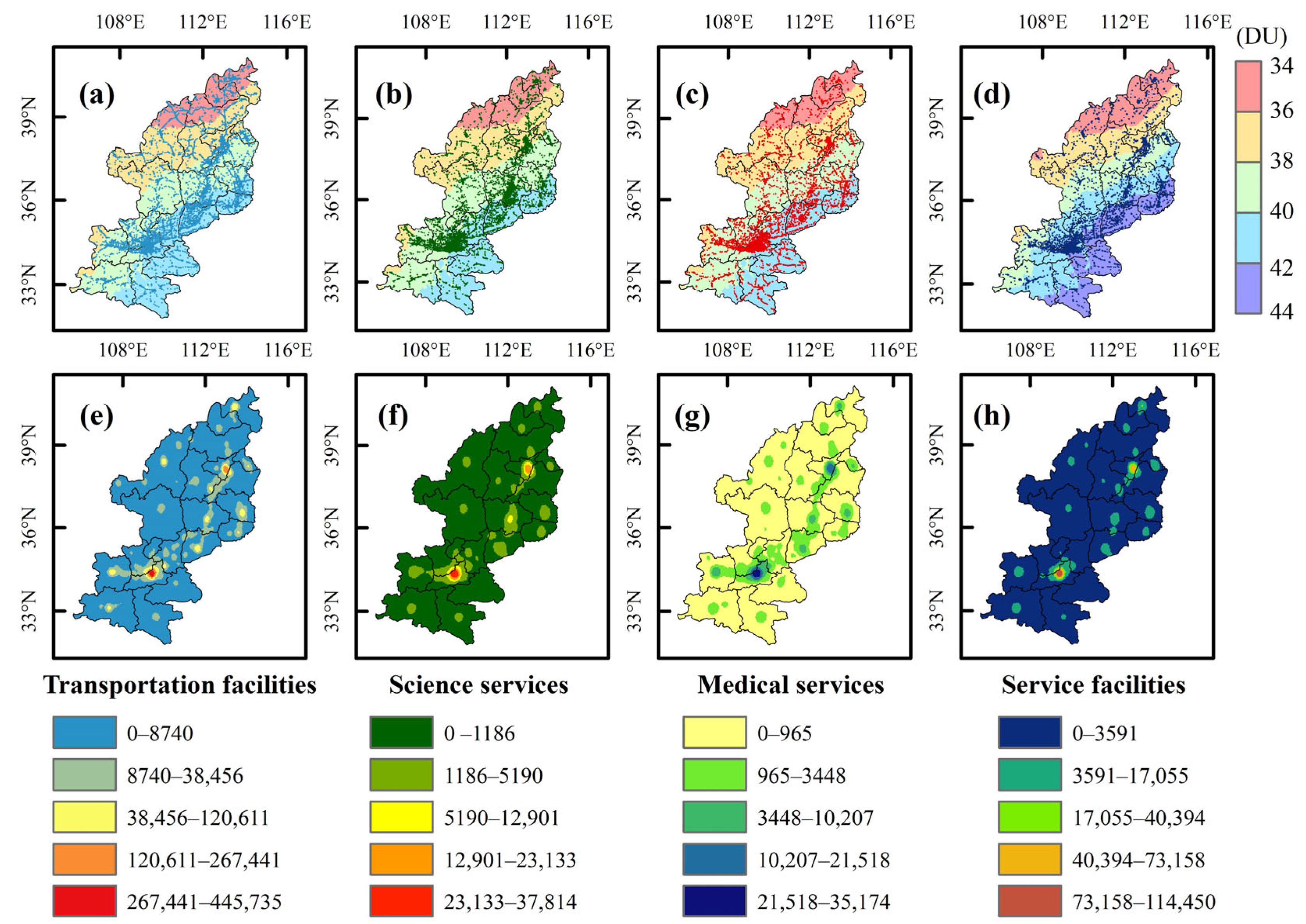
3.3.1. Human Factors

Using the point data of population distribution in the last ten years to make a standard deviation ellipse and center-of-gravity migration trajectory in ArcGIS10.6, the long half-axis of the ellipse indicates the direction of the main population distribution, and the short half-axis indicates the range of the main population distribution. The more significant the difference between the values of the long and short half-axis (the more extensive the flattening rate), the more pronounced the direction of the main population. The center-of-gravity point indicates the center of the whole data. The population center of gravity migration trajectory is observed to be primarily located in the areas adjacent to Yan’an, Weinan, and Linfen from 2013 to 2022, as depicted in Figure 8. Specifically, the center of gravity of the population in 2017–2019 migrated a shorter distance eastward compared to 2013–2016, and migrated a long distance to the southwest from 2020 to 2022. The area of the standard deviation ellipse increased annually from 2015 to 2019. However, post 2020, there was a slight reduction in the area of the standard deviation ellipse, indicating a higher degree of spatial discreteness among population patches within the study area between 2015 and 2019, and this period exhibited an inclination towards expansion into a larger region. The shrinking trend in the standard deviation ellipse behind 2020 may be related to the epidemic’s impact on people’s daily productive lives.

Figure 9 shows the clustering characteristics of the tropospheric ozone column concentrations in the Qin–Jin region concerning the four kernel density analyses of human transportation activities, scientific services, medical services, and service facilities. The spatial pattern is that the degree of clustering is also higher where the population size is high, and the areas with a high degree of clustering are distributed in the narrow strip in the middle of this study. The clustering characteristics after POI kernel density analysis largely overlap with the spatial distribution characteristics of the population in Figure 8. Biomass burning and coal combustion sources contribute prominently in the fall and winter, industrial and dust sources contribute in the spring and summer, and motor vehicle sources contribute relatively significantly in the summer and fall. However, not all urban areas have the highest tropospheric ozone concentrations, suggesting that human activities play an essential role and other factors also influence changes in ozone concentrations. China was identified as the predominant source of CO, NO_X, NMVOC, and CH₄ emissions in Asia in 2008, and the growth rate of these emissions in China surpasses those of any other to its ongoing development, escalating energy consumption, economic activities, and infrastructure expansion [33].

3.3.2. Natural Factors

As seen in

Table 4. Fit coefficients of ozone and natural factors under the GTWR model.

Variables	Pearson	VIF	Min.	Max.	Median	Average
NDVI	0.664 **	3.090	−0.713	0.813	0.034	0.044
TPW	0.811 **	9.017	−3.514	4.124	0.428	0.508
TEM	0.891 **	9.788	−3.883	4.302	0.309	0.302
PS	0.008 *	1.261	−2.993	1.266	0.025	0.041
LI	−0.796 **	5.557	−2.709	4.809	−0.010	−0.012
RH	0.206 **	2.842	−2.593	0.984	−0.240	−0.295

** Significantly correlated at the 0.01 level (bilateral); * significantly correlated at the 0.05 level (bilateral).

, based on the GTWR model [34], after standardizing the influencing factors in the covariance test according to uniform standards, the Variance Inflation Factor (VIF) values were found to be less than 10. This indicates that the independent variables are not correlated with each other and do not introduce model instability, due to multicollinearity issues. In Pearson’s test, vegetation cover (NDVI), precipitable water (TPW), temperature (TEM), lift index (LI), and relative humidity (RH) were significantly correlated with ozone at p < 0.01, and barometric pressure (PS) was significantly correlated with ozone at p < 0.05, which indicates that the selected indicators are meaningful. The GTWR was run with a goodness-of-fit R² of 0.964 and a bandwidth of 1.398, indicating a good fit. Based on the mean regression coefficient values of the variables in the table, it can be seen that vegetation cover (NDVI), precipitable water (TPW), temperature (TEM), and barometric pressure (PS) are positively correlated with ozone concentration, while lift index (LI) and relative humidity (RH) are negatively correlated with ozone concentration. Vegetation cover (NDVI) has a small range of variation in ozone correlation coefficients, and precipitable water (TPW), temperature (TEM), and lift index (LI) have an extensive range of variation in ozone correlation coefficients. The distribution of cities experiencing more pronounced ozone increases is dispersed, attributed to intricate meteorological influences [9].

Figure 10 is a visual representation of the GTWR model for the regression coefficients of the natural factors. The NDVI index exhibited higher values in southeast Qin–Jin compared to northwest, with the summer NDVI index ranging from −0.037 to 0.92 and the ozone-NDVI regression coefficients ranging from −0.14 to 0.72. A negative ozone–vegetation correlation was predominantly observed in Lvliang and Weinan cities, accounting for approximately 24.23% of the total study area. It is shown that the interaction between ozone and vegetation in most parts of Qin–Jin eventually leads to an increase in tropospheric ozone concentration because vegetation influences ozone production through the emission of volatile organic compounds (BVOCS) and also participates in the ozone deposition process through the uptake of leaf stomata, while prolonged exposure to ozone concentrations induces a linear decrease in the emission of isoprene from vegetation, which alters the concentration of ozone precursors and thus influences ozone production (Figure 10a). The Qin–Jin region exhibits a distinct seasonal pattern in terms of precipitation, with summer rainfall being significantly more pronounced than that in spring and fall. The negative correlation between precipitable water and ozone was primarily observed in Xianyang, Xi’an, Shangzhou, Baoji, Ankang, and Hanzhong, encompassing approximately 34.72% of the total study area. In the northern region of the study area, characterized by low precipitation levels, a weak positive correlation was found between ozone and precipitation, which suggests that the limited rainfall did not effectively scavenge pollutants (Figure 10b). The highest summer temperatures and lowest winter temperatures are found in the Qin–Jin area, with temperatures in the range of 279.28–287.45 K in spring and fall, and the areas of high temperatures are mainly located in the central and southern parts of the study area. The regression coefficients of temperature and ozone were all positive, and the positive correlation between increasing temperature and ozone concentration was more pronounced in the southeastern region of the study area. The underlying reason for this phenomenon lies in the fact that temperature serves as an indicator to some extent for solar radiation intensity, which directly influences both ozone production and depletion rates (Figure 10c).

The air pressure gradually increased from west to east within the study area, and the regression coefficients of ozone and air pressure ranged from −0.61 to 0.27. However, compared to the other five natural factors, air has a weak correlation with ozone (Figure 10d). The uplift index distribution in the study area follows a seasonal pattern, with winter exhibiting the highest values, followed by autumn, spring, and summer, and there is a gradual increase in the uplift index from southwest to northeast. The ozone and lifting index exhibit a strong positive correlation in 99.47% of the regions, with Yan’an, Tongchuan, and Weinan displaying the highest correlation coefficients. The lifting index is utilized to characterize atmospheric stability and the probability of intense convective weather, as an unstable atmospheric structure often exhibits a higher likelihood of inversions that impede the vertical transport of surface gases (Figure 10e). The spatial and temporal distribution of relative humidity in the study area are roughly the same as those of precipitable water. The negative correlation region between relative humidity and ozone is 42 in eastern Shanxi Province and Baoji City in Shaanxi Province. This relationship leads to a reduction in the concentration of ozone columns due to its dilution and depositional effects on ozone (Figure 10f).

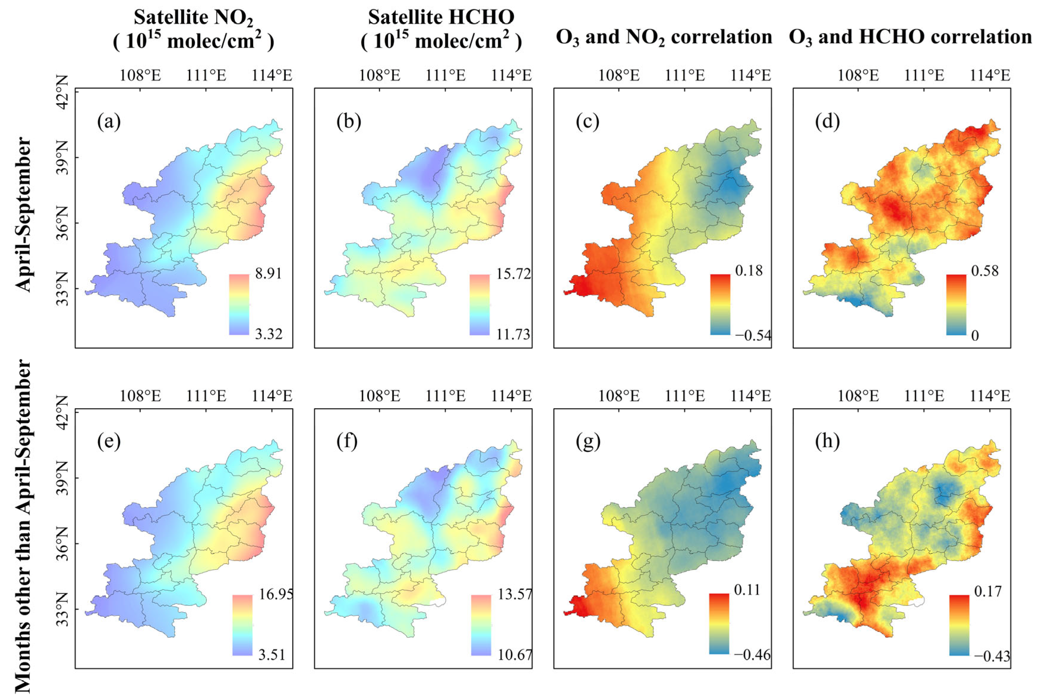
3.3.3. Ozone Precursors

In this study, VOC_s/NO_x from near-surface observations are approximated by replacing them with HCHO/NO₂ data based on OMI satellite measurements [35]. As shown in Figure 11, the overall spatial distribution of tropospheric NO₂ shows a gradual increase from southwest to northeast, and the heavily polluted areas are mainly located in Yangquan, Jinzhong, Changzhi, and Jincheng. The spatial distribution of tropospheric HCHO in April–September and other months is different, and Hanzhong City has a higher HCHO in April–September than in other months. Tropospheric NO₂ varied from 3.32 to 8.91 × 10¹⁵ molec/cm² and 3.51 to 16.95 × 10¹⁵ molec/cm² during the high-pollution period (April–September) and other months, respectively. Tropospheric HCHO varies from 11.73 to 15.72 × 10¹⁵ molec/cm² and 10.67 to 13.57 × 10¹⁵ molec/cm² during the high-pollution period (April–September) and other months, respectively. NO₂ has a large area of low concentration from April to September due to the high surface temperature and thin atmospheric stabilization layer at this time, coupled with the fact that there is no heating demand compared to the other months, which reduces NO₂ emissions and thus leads to a decrease in its concentration. In contrast, HCHO has a large area of high concentrations from April to September, with significant increases in all regions except for Elmwood, which has a minor increase compared to other months. Therefore, VOCs in the Qin–Jin region significantly impact the high-ozone period more than NOx.

In April–September, the spatial distribution correlations of O₃ with NO₂ and HCHO ranged from −0.54 to 0.18 (Figure 11c) and 0 to 0.58 (Figure 11d), respectively. In months other than April–September, the spatial distribution correlations of O₃ with NO₂ and HCHO ranged from −0.46 to 0.11 (Figure 11g) and −0.43 to 0.17 (Figure 11h), respectively. Among them, the range of correlation between O₃ and NO₂ in April–September was broader than in other months. The area of positive correlation was also increased, and the positive correlation area was mainly distributed in Baoji and Hanzhong cities. O₃ and HCHO were positively correlated from April to September, especially in central Yan’an, where the positive correlation had the most significant impact. O₃ and HCHO were negatively correlated in 85.03% of the region’s area for months other than April–September. Therefore, we concluded that emissions of VOCs accelerated ozone production in April–September in the Qin–Jin region, and emissions of NOx suppressed ozone production in most areas. In contrast, VOCs inhibited ozone production in most parts of the study area in months other than April–September.

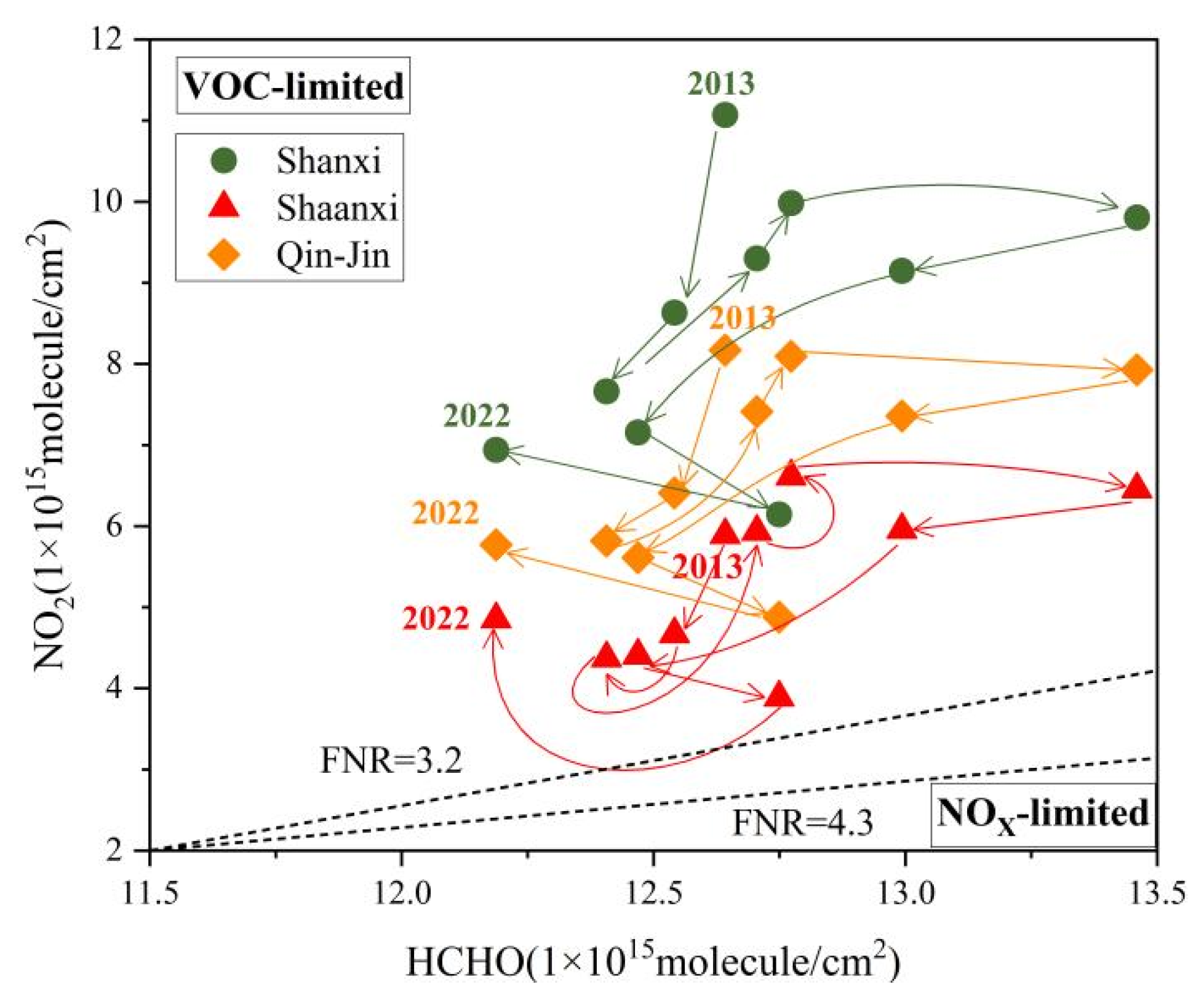
3.4. Control Based on Ozone Sensitivity

In numerous urban areas, many air pollutants, such as SO₂, NO₂, CO, PM_2.5, and PM₁₀, have declined in recent years; however, concentrations of O₃ are experiencing an upward trend [36]. Similar phenomena have been observed in other countries, with the implementation of VOC reduction strategies in the United States in the 1980s and 1990s mitigating ozone pollution in Los Angeles and New York. However, ozone levels in other parts of the United States remain high [37]. Therefore, reducing ozone concentration has become a priority in China’s air quality control strategy [38]. The temporal trends of the ozone generation sensitivity indicator FNR in Shanxi Province, Shaanxi Province, and the entire Qin–Jin region from 2013 to 2022 are shown in Figure 12. This figure shows the changing pattern of FNR values for ozone generation: Shaanxi Province > Qin–Jin region > Shanxi Province. Moreover, all annual average FNRs are distributed within the VOC_s control area. The minimum value of annual average FNR occurred in Shanxi Province in 2013 (1.15), the minimum value of annual average FNR occurred in Shaanxi Province in 2017 (1.91), and the maximum value of annual average FNR occurred in 2021 for both Shaanxi Province and Shanxi Province.

Longer NO_X lifetimes and low OH and RO₂ radical concentrations will lead to a VOC-limited winter in most parts of China [39]. Therefore, the primary period for ozone control in the study area spans from April to September, as summer represents a critical phase during which meteorological factors can exploit the potential for ozone formation [40].

Figure 13 illustrates the spatial distribution of tropospheric ozone generation sensitivity FNR in the Qin–Jin area from April to September between 2013 and 2022. The results indicate that VOC_s dominate the control of tropospheric ozone generation, accounting for 78.46%, 68.89%, 56.58%, 58.84%, 60.50%, and 96.55% of the study area in April, May, August, and September over the past, and only in June did NO_x contribute to a mere fraction (2.380%) of this control. FNR values gradually increased from northeast to southwest. The northern regions of China, characterized by cold conditions and the prevalence of the titration effect resulting from elevated NO₂ emissions, act to suppress ozone production. The fluctuations in FNR observed during periods of high ozone pollution within the study area suggest that the focus has shifted from NO_x to VOC_s in urban regions, with formaldehyde potentially playing a pivotal role in reducing ozone levels [41]. However, synergistic control of NO_x and VOC_s is still required in certain regions during periods of high pollution levels, with a particular focus on the southern Shaanxi Province. Jin and Holloway concluded that in China, VOC_s-limiting areas are widespread in mega-city clusters (the North China Plain, the Yangtze Delta, and the Pearl River Delta) and are concentrated in developed cities (e.g., Chengdu, Chongqing, Xi’an, and Wuhan), and NOx-limiting areas are concentrated in much of the remainder of China [10].

4. Conclusions

Spatially, ozone in the Qin–Jin region exhibited a spatial gradient of increasing concentration from northwest to southeast. The Slope indicated a slight upward trend in ozone levels across the study area (0~0.079). Temporally, the monthly average ozone trend is monomodal, with ozone concentration values much greater in April–September than in other months. The seasonal order of ozone concentrations was summer > spring > fall > winter, and no weekend effect was observed within the study area. In addition, ozone is predicted to average 36.57, 50.88, 34.29, and 30.10 DU in spring, summer, fall, and winter, respectively, in 2023.

Based on the BenMap-CE model, it was estimated that the average values of all-cause premature deaths and economic losses in Shanxi Province were 4591 and 4214 persons and 43.30 and 51.30 billion yuan in 2019 and 2021, and the average values of all-cause premature deaths and economic losses in Shaanxi Province were 2498 and 1535 persons and 23.50 and 18.70 billion yuan in 2019 and 2021, respectively. The study area had more premature deaths due to cardiovascular diseases than respiratory diseases.

We consider transportation emissions to be the most significant contributor to anthropogenic emissions of ozone, followed by services, with both scientific and medical services contributing less. The clustering characteristics of human activities affect high and low tropospheric ozone concentrations but do not entirely overlap. The correlation between natural factors and ozone has the following order: temperature-positive correlation, followed by precipitable water, vegetation cover, and relative humidity. Conversely, the uplift index shows a negative correlation with ozone levels. Barometric pressure, on the other hand, demonstrates limited or no significant correlation. During April and September, emissions of VOCs accelerated ozone production, and emissions of NOx suppressed ozone production over most of the area. In months other than April–September, emissions of both VOCs and NOx suppressed ozone production in most parts of the study area.

Based on these results, we provide valuable information on ozone pollution in the Qin–Jin region from 2013 to 2022, and these findings can provide a valuable reference for understanding ozone changes around the world. For the study area, the period of high ozone pollution is primarily a VOC control area, and the synergistic control of NOx and VOCs is secondary. In addition, effective reduction in the health impacts of ozone pollution requires promoting healthy urban environments through urbanization planning and management, early warning and publicity, and the awareness and protection of residents.

5. Limitations and Prospects

This study utilized multivariate ozone data, meteorological factors, socioeconomic indicators, and population health statistics to investigate Qin–Jin’s spatiotemporal patterns of ozone pollution from 2013 to 2022. Additionally, it elucidated the influencing factors on ozone levels and evaluated the health and economic impacts of ozone pollution in China based on simulations of ozone concentrations. This paper needs further refinement in terms of content and methodology.

The meteorological factors considered in the study of factors influencing ozone pollution in the study area need to be more comprehensive, and all meteorological factors should be synthesized to influence the complexity of ozone concentration.

For the health risk evaluation of ozone, attribute characteristics such as gender, age, health status, education level, and inflation and exchange rates were not taken into account. Therefore, it is impossible to assess ozone pollution’s health effects more comprehensively and accurately.

References

1. Chameides, W.; Walker, J.C.G. A photochemical theory of tropospheric ozone. J. Geophys. Res. 1973, 78, 8751–8760. [Google Scholar] [CrossRef]
2. Fang, Y.; Naik, V.; Horowitz, L.; Mauzerall, D. Air pollution and associated human mortality: The role of air pollutant emissions, climate change and methane concentration increases from the preindustrial period to present. Atmos. Chem. Phys. 2013, 13, 1377–1394. [Google Scholar] [CrossRef]
3. Booker, F.; Muntifering, R.; McGrath, M.; Burkey, K.; Decoteau, D.; Fiscus, E.; Manning, W.; Krupa, S.; Chappelka, A.; Grantz, D. The ozone component of global change: Potential effects on agricultural and horticultural plant yield, product quality and interactions with invasive species. J. Integr. Plant Biol. 2009, 51, 337–351. [Google Scholar] [CrossRef] [PubMed]
4. Lim, C.C.; Hayes, R.B.; Ahn, J.; Shao, Y.; Silverman, D.T.; Jones, R.R.; Garcia, C.; Bell, M.L.; Thurston, G.D. Long-Term Exposure to Ozone and Cause-Specific Mortality Risk in the United States. Am. J. Respir. Crit. Care Med. 2019, 200, 1022–1031. [Google Scholar] [CrossRef]
5. Li, K.; Jacob, D.J.; Liao, H.; Shen, L.; Zhang, Q.; Bates, K.H. Anthropogenic drivers of 2013–2017 trends in summer surface ozone in China. Proc. Natl. Acad. Sci. USA 2019, 116, 422–427. [Google Scholar] [CrossRef] [PubMed]
6. Lu, X.; Hong, J.; Zhang, L.; Cooper, O.R.; Schultz, M.G.; Xu, X.; Wang, T.; Gao, M.; Zhao, Y.; Zhang, Y. Severe Surface Ozone Pollution in China: A Global Perspective. Environ. Sci. Technol. Lett. 2018, 5, 487–494. [Google Scholar] [CrossRef]
7. Dai, H.; Zhu, J.; Liao, H.; Li, J.; Liang, M.; Yang, Y.; Yue, X. Co-occurrence of ozone and PM2.5 pollution in the Yangtze River Delta over 2013–2019: Spatiotemporal distribution and meteorological conditions. Atmos. Res. 2021, 249, 105363. [Google Scholar] [CrossRef]
8. Derwent, R.G.; Utembe, S.R.; Jenkin, M.E.; Shallcross, D.E. Tropospheric ozone production regions and the intercontinental origins of surface ozone over Europe. Atmos. Environ. 2015, 112, 216–224. [Google Scholar] [CrossRef]
9. Wang, T.; Xue, L.; Brimblecombe, P.; Lam, Y.F.; Li, L.; Zhang, L. Ozone pollution in China: A review of concentrations, meteorological influences, chemical precursors, and effects. Sci. Total Environ. 2017, 575, 1582–1596. [Google Scholar] [CrossRef]
10. Jin, X.; Holloway, T. Spatial and temporal variability of ozone sensitivity over China observed from the Ozone Monitoring Instrument. J. Geophys. Res. Atmos. 2015, 120, 7229–7246. [Google Scholar] [CrossRef]
11. Li, K.; Jacob, D.J.; Shen, L.; Lu, X.; De Smedt, I.; Liao, H. Increases in surface ozone pollution in China from 2013 to 2019: Anthropogenic and meteorological influences. Atmos. Chem. Phys. 2020, 20, 11423–11433. [Google Scholar] [CrossRef]
12. Liu, Y.; Wang, T. Worsening urban ozone pollution in China from 2013 to 2017—Part 2: The effects of emission changes and implications for multi-pollutant control. Atmos. Chem. Phys. 2020, 20, 6323–6337. [Google Scholar] [CrossRef]
13. Gong, S.; Zhang, L.; Liu, C.; Lu, S.; Pan, W.; Zhang, Y. Multi-scale analysis of the impacts of meteorology and emissions on PM2.5 and O3 trends at various regions in China from 2013 to 2020 2. Key weather elements and emissions. Sci. Total Environ. 2022, 824, 153847. [Google Scholar] [CrossRef] [PubMed]
14. Wang, W.; van der A, R.; Ding, J.; van Weele, M.; Cheng, T. Spatial and temporal changes of the ozone sensitivity in China based on satellite and ground-based observations. Atmos. Chem. Phys. 2021, 21, 7253–7269. [Google Scholar] [CrossRef]
15. Cao, J.-J.; Zhang, T.; Chow, J.C.; Watson, J.G.; Wu, F.; Li, H. Characterization of Atmospheric Ammonia over Xi’an, China. Aerosol Air Qual. Res. 2009, 9, 277–289. [Google Scholar] [CrossRef]
16. Yan, K.; Yang, C.A.-O.; Zhang, H.; Ye, D.; Liu, S.; Chang, J.; Jiang, M.; Zhao, M.; Fang, Y. Impact of the zero-mark-up drug policy on drug-related expenditures and use in public hospitals, 2016–2018: An interrupted time series study in Shaanxi. BMJ Open 2020, 10, e037034. [Google Scholar] [CrossRef] [PubMed]
17. Breiman, L.; Friedman, J.H.; Olshen, R.A.; Stone, C.J.J.B. Classification and Regression Trees. Biometrics 1984, 40, 874. [Google Scholar]
18. Breiman, L. Random Forests. Mach. Learn. 2001, 45, 5–32. [Google Scholar] [CrossRef]
19. Turner, M.; Jerrett, M.; Pope, C.; Krewski, D.; Gapstur, S.; Diver, W.; Beckerman, B.; Marshall, J.; Su, J.; Crouse, D.; et al. Long-Term Ozone Exposure and Mortality in a Large Prospective Study. Am. J. Respir. Crit. Care Med. 2015, 193, 1134–1142. [Google Scholar] [CrossRef]
20. Yin, P.; Chen, R.; Wang, L.; Meng, X.; Liu, C.; Niu, Y.; Lin, Z.; Liu, Y.; Liu, J.; Qi, J.; et al. Ambient Ozone Pollution and Daily Mortality: A Nationwide Study in 272 Chinese Cities. Environ. Health Perspect 2017, 125, 117006. [Google Scholar] [CrossRef]
21. Shang, Y.; Sun, Z.; Cao, J.; Wang, X.; Zhong, L.; Bi, X.; Li, H.; Liu, W.; Zhu, T.; Huang, W. Systematic review of Chinese studies of short-term exposure to air pollution and daily mortality. Environ. Int. 2013, 54, 100–111. [Google Scholar] [CrossRef] [PubMed]
22. Huang, B.; Wu, B.; Barry, M. Geographically and temporally weighted regression for modeling spatio-temporal variation in house prices. Int. J. Geogr. Inf. Sci. 2010, 24, 383–401. [Google Scholar] [CrossRef]
23. Wahiduzzaman, M.; Yeasmin, A. A kernel density estimation approach of North Indian Ocean tropical cyclone formation and the association with convective available potential energy and equivalent potential temperature. Meteorol. Atmos. Phys. 2020, 132, 603–612. [Google Scholar] [CrossRef]
24. Ren, J.; Guo, F.; Xie, S. Diagnosing ozone–NOx–VOC sensitivity and revealing causes of ozone increases in China based on 2013–2021 satellite retrievals. Atmos. Chem. Phys. 2022, 22, 15035–15047. [Google Scholar] [CrossRef]
25. Li, Y. Study on the Temporal and Spatial Variations of Tropospheric Ozone and Its Impacting Factors. Master’s Thesis, Lanzhou University, Lanzhou, China, 2018. Available online: https://kns.cnki.net/kcms2/article/abstract?v=IUBLoWpfHZHeJTUH6yoL7bBmJ2qt_mrqLkUkxaC_XDjU2yL8phg_IOQiOSr23ZKnTFEDsJt8HesRk4G-4mMHFWxhUsW-KiJOnGdHaqZrhYplS-KKQrvRtI84Fb4du2zml_EtxqayB8g=&uniplatform=NZKPT&language=CHS (accessed on 1 July 2023).
26. Song, S.; Fan, M.; Tao, J.; Chen, S.; Gu, J.; Han, Z.; Liang, X.; Lu, X.; Wang, T.; Zhang, Y. Estimating ground-level ozone concentration in China using ensemble learning methods. J. Remote Sens. 2023, 27, 1792–1806. [Google Scholar]
27. Zhao, S.; Yin, D.; Yu, Y.; Kang, S.; Qin, D.; Dong, L. PM2.5 and O3 pollution during 2015–2019 over 367 Chinese cities: Spatiotemporal variations, meteorological and topographical impacts. Environ. Pollut. 2020, 264, 114694. [Google Scholar] [CrossRef]
28. Cleveland, W.S.; Graedel, T.E.; Kleiner, B.; Warner, J.L. Sunday and Workday Variations in Photochemical Air Pollutants in New Jersey and New York. Science 1974, 186, 1037–1038. [Google Scholar] [CrossRef]
29. Zhao, X.; Zhou, W.; Han, L. Human activities and urban air pollution in Chinese mega city: An insight of ozone weekend effect in Beijing. Phys. Chem. Earth Parts A/B/C 2019, 110, 109–116. [Google Scholar] [CrossRef]
30. Stavrakou, T.; Müller, J.F.; Bauwens, M.; De Smedt, I.; Van Roozendael, M.; Guenther, A.; Wild, M.; Xia, X. Isoprene emissions over Asia 1979&ndash;2012: Impact of climate and land-use changes. Atmos. Chem. Phys. 2014, 14, 4587–4605. [Google Scholar] [CrossRef]
31. Jonson, J.E.; Simpson, D.; Fagerli, H.; Solberg, S. Can we explain the trends in European ozone levels? Atmos. Chem. Phys. 2006, 6, 51–66. [Google Scholar] [CrossRef]
32. Yin, P.; Brauer, M.; Cohen, A.J.; Wang, H.; Li, J.; Burnett, R.T.; Stanaway, J.D.; Causey, K.; Larson, S.; Godwin, W.; et al. The effect of air pollution on deaths, disease burden, and life expectancy across China and its provinces, 1990–2017: An analysis for the Global Burden of Disease Study 2017. Lancet Planet. Health 2020, 4, e386–e398. [Google Scholar] [CrossRef] [PubMed]
33. Kurokawa, J.; Ohara, T.; Morikawa, T.; Hanayama, S.; Janssens-Maenhout, G.; Fukui, T.; Kawashima, K.; Akimoto, H. Emissions of air pollutants and greenhouse gases over Asian regions during 2000–2008: Regional Emission inventory in ASia (REAS) version 2. Atmos. Chem. Phys. 2013, 13, 11019–11058. [Google Scholar] [CrossRef]
34. Lei, S.; Ju, T.; Li, B.; Xia, X.; Huang, C.; Zhang, J.; Li, C. Analysis of Remote Sensing Monitoring of Atmospheric Ozone in Japan from 2010 to 2021. Water Air Soil Pollut. 2023, 234, 562. [Google Scholar] [CrossRef]
35. Jin, X.; Fiore, A.M.; Murray, L.T.; Valin, L.C.; Lamsal, L.N.; Duncan, B.N.; Folkert Boersma, K.; de Smedt, I.; Abad, G.G.; Chance, K.; et al. Evaluating a Space-Based Indicator of Surface Ozone-NOx-VOC Sensitivity Over Midlatitude Source Regions and Application to Decadal Trends. J. Geophys. Res. Atmos. 2017, 122, 439–461. [Google Scholar] [CrossRef] [PubMed]
36. Zeng, Y.; Cao, Y.; Qiao, X.; Seyler, B.C.; Tang, Y. Air pollution reduction in China: Recent success but great challenge for the future. Sci. Total Environ. 2019, 663, 329–337. [Google Scholar] [CrossRef] [PubMed]
37. Jacob, D.J. Introduction to Atmospheric Chemistry; Princeton University Press: Princeton, NJ, USA, 1999. [Google Scholar]
38. Cheng, L.; Wang, S.; Gong, Z.; Li, H.; Yang, Q.; Wang, Y. Regionalization based on spatial and seasonal variation in ground-level ozone concentrations across China. J. Environ. Sci. 2018, 67, 179–190. [Google Scholar] [CrossRef]
39. Shah, V.; Jacob, D.J.; Li, K.; Silvern, R.F.; Zhai, S.; Liu, M.; Lin, J.; Zhang, Q. Effect of changing NOx lifetime on the seasonality and long-term trends of satellite-observed tropospheric NO2 columns over China. Atmos. Chem. Phys. 2020, 20, 1483–1495. [Google Scholar] [CrossRef]
40. Jin, X.; Fiore, A.; Boersma, K.; De Smedt, I.; Valin, L. Inferring Changes in Summertime Surface Ozone–NOx–VOC Chemistry over U.S. Urban Areas from Two Decades of Satellite and Ground-Based Observations. Environ. Sci. Technol. 2020, 54, 6518–6529. [Google Scholar] [CrossRef]
41. Wasti, S.; Wang, Y. Spatial and temporal analysis of HCHO response to drought in South Korea. Sci. Total Environ. 2022, 852, 158451. [Google Scholar] [CrossRef]
Figure 1. Overview of the study area: (a) elevation map; (b) land use types and administrative divisions.
Sustainability 15 16945 g001
Figure 2. Technology roadmap.
Sustainability 15 16945 g002
Figure 3. (a) Overall spatial distribution of tropospheric ozone column concentration in Qin–Jin region, 2013–2022; (b) Slope past trend analysis; (c) percentage change of tropospheric ozone column concentration and three-value changes. The abbreviation “DU” stands for Dobson Unit.
Sustainability 15 16945 g003
Figure 4. Monthly average spatial distribution of tropospheric ozone column concentrations in Qin–Jin region, 2013–2022.
Sustainability 15 16945 g004
Figure 5. (a) Box plots of monthly O3 concentrations across Qin–Jin area; the relationships between O3 concentrations across four seasons are also given in the subplot. (b) Box plots of weekly O3 concentrations across Qin–Jin area; the relationships between O3 concentrations across workdays and weekends are also given in the subplot.
Sustainability 15 16945 g005
Figure 6. Measured tropospheric ozone column concentrations in the four seasons of 2022 and random forest regression model predictions for 2022 and 2023 of Qin–Jin.
Sustainability 15 16945 g006
Figure 7. The map for visualization of early death values for ozone pollution in the Qin–Jin region. (a) All-cause mortality in 2019; (b) Cardiovascular mortality in 2019; (c) Respiratory mortality in 2019; (d) All-cause mortality in 2021; (e) Cardiovascular mortality in 2021; and (f) Respiratory mortality in 2021.
Sustainability 15 16945 g007
Figure 8. Spatial distribution of population, standard deviation ellipse, and center of gravity migration trajectory in Qin–Jin region.
Sustainability 15 16945 g008
Figure 9. Kernel density estimates for (a,e) transportation facilities, (b,f) scientific services, and (c,g) medical services (d,h) in the Qin–jin area. The upper column shows the relationship between the distribution of POI and tropospheric ozone, the lower column shows the clustering characteristics from the kernel density analysis.
Sustainability 15 16945 g009
Figure 10. The spatial distribution of the regression coefficients of ozone-related natural variables in the GTWR model is shown in the figure. These variables are as follows: (a) vegetation cover, (b) precipitable water, (c) air temperature, (d) barometric pressure, (e) uplift index, and (f) relative humidity.
Sustainability 15 16945 g010
Figure 11. Spatial distribution of ozone precursors during the high-pollution period (April–September) and other months, Pearson correlation analysis map. (a) April–September tropospheric NO2 concentration; (b) April–September tropospheric HCHO concentration; (c) April–September O3-NO2 correlation; (d) April–September O3-HCHO correlation; (e) Tropospheric NO2 concentration other than April–September; (f) Tropospheric HCHO concentration other than April–September; (g) O3-NO2 correlation other than April–September; (h) O3-HCHO correlation other than April–September.
Sustainability 15 16945 g011
Figure 12. Temporal trend of FNR for Qin–Jin region, 2013–2022.
Sustainability 15 16945 g012
Figure 13. Spatial distribution of tropospheric ozone FNR for April–September 2013–2022.
Sustainability 15 16945 g013