Article

Mapping LULC Dynamics and Its Potential Implication on Forest Cover in Malam Jabba Region with Landsat Time Series Imagery and Random Forest Classification

1
Faculty of Geomatics, Lanzhou Jiaotong University, Lanzhou 730070, China
2
National-Local Joint Engineering Research Center of Technologies and Applications for National Geographic, State Monitoring, Lanzhou 730070, China
3
Gansu Provincial Engineering Laboratory for National Geographic State Monitoring, Lanzhou 730070, China
4
Department of Space Sciences, Institute of Space Technology, Islamabad 44000, Pakistan
5
Centre for Water Informatics and Technology, Lahore University of Management Science, Lahore 54792, Pakistan
6
Department of Geology, University of Haripur, Haripur 22610, Pakistan
*
Author to whom correspondence should be addressed.
Sustainability 2023, 15(3), 1858; https://doi.org/10.3390/su15031858
Submission received: 27 November 2022 / Revised: 23 December 2022 / Accepted: 11 January 2023 / Published: 18 January 2023
(This article belongs to the Section Sustainability in Geographic Science)

Abstract

:
Pakistan has an annual deforestation rate of 4.6% which is the second highest in Asia. It has been described by the Food and Agriculture Organization (FAO) that the deforestation rate increased from 1.8–2.2% within two decades (1980–2000 and 2000–2010). KPK (Khyber Pakhtunkhwa), Pakistan’s northwestern province, holds 31% of the country’s total forest resources, the majority of which are natural forests. The Malam Jabba region, known for its agro-forestry practices, has undergone significant changes in its agricultural, forestry, and urban development. Agricultural and built-up land increased by 77.6% in the last four decades, and significant changes in land cover especially loss in forest, woodland, and agricultural land were observed due to flood disasters since 1980. For assessing and interpreting land-cover dynamics, particularly for changes in natural resources such as evergreen forest cover, remote sensing images are valuable assets. This study proposes a framework to assess the changes in vegetation cover in the Malam Jabba region during the past four decades with Landsat time series data. The random forest classifier (RF) was used to analyze the forest, woodland, and other land cover changes over the past four decades. Landsat MMS, TM, ETM+, and OLI satellite images were used as inputs for the random forest (RF) classifier. The vegetation cover change for each period was calculated from the pixels using vegetation indices such as NDVI, SAVI, and VCI. The results show that Malam Jabba’s total forest land area in 1980 was about 236 km2 and shrank to 152 km2 by 2020. The overall loss rate of evergreen forests was 35.3 percent. The mean forest cover loss rate occurred at 2.1 km2/year from 1980 to 2020. The area of woodland forest decreased by 87 km2 (25.43 percent) between 1980 and 2020. Other landcover increased by 121% and covered a total area of 178 km2. The overall accuracy was about 94% and the value of the kappa coefficient was 0.92 for the change in forest and woodland cover. In conclusion, this study can be beneficial to researchers and decision makers who are enthusiastic about using remote sensing for monitoring and planning the development of LULC at the regional and global scales.

1. Introduction

Since the beginning of the 21st century, anthropogenic land use and land cover transformations have developed into a major source of worldwide ecological concerns. This has put pressure on the natural ecosystem, hence degrading green lands such as forests and other resources [1]. The significance of forest cover is crucial in controlling the Earth’s temperature and precipitation, preserving soil quality, controlling erosion, reducing floods, and capturing carbon dioxide [2]. Being the second-largest source of carbon dioxide emissions (10–25 percent globally), deforestation has wide-ranging environmental and socioeconomic implications [3,4]. Deforestation and forest exploitation can result in the release of CO2 upwards into the Earth’s atmosphere, affecting the global climate and influencing ecological change [5].
Dense trees occupying areas larger than 5 hectares in size, with trees larger than 5 m in height, and covering no less than 10% of the canopy is known as forest land [6]. This excludes most agricultural land and densely populated areas [7]. An area is classified as “Other woodland” if it contains more than 0.5 hectares and has a canopy cover of 5–10 percent or has trees taller than 5 m or a total cover of bushes, shrubs, and trees larger than 10 percent. It excludes area which is primarily used for agricultural purposes or for urban purposes. Shrubland, scattered woody trees, grassland, barren land, agricultural land, and others are defined as other land cover [8].
Deforestation is the process of converting forest land into another type of usage or reducing the tree canopy permanently below a level of 10% [7]. Disturbance, overuse, other anthropogenic activities, or shifting environmental circumstances, all contribute to deforestation when forest cover is reduced to less than 10% [9]. For this, reforestation or afforestation are highly needed. Both reforestation and afforestation are changes in land use, although only afforested land has never had forest before. In the process of reforestation, the land is transformed from a non-forest to a forest area by means of planned sowing on the ground that had previously been used for other purposes [7].
There were more than 3.95 billion hectares of forest cover globally in 2005. Among them, 36 percent was natural forest, 53 percent was modified, 7 percent was semi-natural, and 3 percent was plantation [10]. Pakistan is Asia’s second-highest deforestation hotspot (4.6 percent annually) after Indonesia, according to the World Resources Institute. As a result, the country’s forest resources are being overexploited [11].
Natural resources management, environmental conservation, and other fields of study rely heavily on Earth Observation satellite data with high to moderate resolution. In the early 1970s, the emergence of geographic information systems (GIS) and remote sensing (RS) became crucial for studying global environmental studies [12]. The temporal and geographical change in resources over time and land use and land cover (LULC) changes can be well analyzed using satellite data and GIS techniques [13].
This provides a powerful tool for assessing ecosystem stress, detecting changes in forest cover, and making informed management and planning decisions [14]. However, the quality of satellite images can be adversely affected by factors such as terrain impact and atmospheric influence, which can lead to increased inaccuracy in land cover analysis. In the evaluation and assessment of land cover, different corrections such as atmospheric radiometric and topographic corrections are critical when using multi-sensor, multi-temporal, and multi-spectral images. The Landsat imagery archive (Landsat 1–8 from 1972 to 2020) is one of the most frequently used products for many uses in agriculture and ecology, such as multi-spectral and time series satellite image classifications and mapping of natural resources management. Various vegetation indexes, such as NDVI, VCP, and SAVI, have the potential for a more precise result of classifications and the assessment of vegetation cover with digital elevation models [15].
Maximum likelihood [16], random forest (RF), deep learning [17,18], artificial neural networks (ANN), conventional neural networks [19], and fuzzy classification [20] are some of the classification techniques used for land use and land cover (LULC) mapping [21].
Among these classifiers, support vector machine [22] and random forest [23,24] have gained attention and evolved into two excellent choices in LULC mapping due to their improved accuracy and efficiency, and comparatively low computational process [25]. Although deep learning and deep transfer learning approaches have been efficient computational strategies in machine learning in recent years, they require a large amount of data and restrict intricate calculations in the cloud platform.
Random forest is a classification and regression tree-based technique. However, in land cover classification, the random forest is predominantly used with NDVI [26] and multispectral and hyperspectral images [27]. In order to more precisely map land cover from satellite images, the random forest (RF) approach was subsequently proposed and implemented [28]. The process of feature generation is a crucial one in many machine learning applications. The mean decline in accuracy (MDA) and the mean drop in the Gini index (MGI) are two measures of the variables’ relative importance that are considered by RF algorithms. The method is put to use in order to identify the most essential features among a large number of candidates in order to construct reliable learning models [29]. Therefore, knowing which spectral, spatial, and temporal characteristics are most important in the classification method and process is as important as getting more precise maps.
Recently, researchers have used satellite-based images to accurately measure and review land use alteration, evaluate land degradation, and monitor land use [30,31,32]. Landsat data are also utilized to investigate land degradation issues such as desertification and deforestation. In three distinct zones in the Swat District, including agro-forest, alpine forest, and scrub forest, yearly deforestation rates of 1.85 percent, 1.28 percent, and 0.80 percent were recorded [33,34]. The northern region of Malam Jabba, Swat District, KPK, Pakistan, was chosen as a case study since it is the most severely affected by vegetation loss caused by anthropogenic and natural sources at the regional level. This land cover classification is performed on Landsat satellite images as it has the advantage of long-term data availability compared with some recent satellite missions. Assessing the urban and agricultural land cover impact on forest land cover is critical. We must evaluate the existing patterns of land use as well as how and why land should be managed and reviewed in order to have a sustainable management practice [33].
In this research, the Malam Jabba region was considered because it contains the maximum cover of coniferous forest in the region. The primary objectives within the context of the current study are (i) to investigate the efficacy of hybrid models for the LULC and its impact on the forest cover area in the research region, and (ii) to create spatial maps utilizing the presented methodologies to pinpoint the most pressing hotspots in need of urgent action. We used the random forest procedure using feature collection because of its appealing abilities, including high precision and robustness over clustering the training data. These findings confirmed the importance of spectral bands, vegetation indices, and DEM in LULC mapping. For data sets with a large number of variables, it is vital to choose the most relevant ones [35,36]. The spatial and temporal data analysis was conducted from 1980 to 2020 with a five-year gap. Each Landsat image was classified as forest, woodland, and other land cover types using the random forest classifier. The training and validation points were created and used for the kappa coefficient and error matrix to assess the accuracy of image classification. In order to offer a current overview of the state of forest resources in the region and the dynamics in deforestation rates, we quantified the rate and potential differences and contrasted them with the other research results and statistics. The information presented in this research will be a great help in the future for guiding future efforts to sustainably manage the forest ecosystem.

2. Materials and Methods

2.1. Study Area

The total area comprising the Swat district is 5037 km2 and it has a population of nearly 1.5 million. This district has a wide range of biological, socioeconomic, and biophysical features, as well as vast and diverse hills and valleys. The Swat district’s population is becoming increasingly cognizant of environmental issues, which has resulted in increased afforestation efforts and forest growth. The Malam Jabba region, 34°47′57″ north, 72°34′19″ east, is the site of the investigation. The hill station of Malam Jabba is located in the Hindu Kush Mountains.
Crops and pine forests make up the majority of vegetative cover in Malam Jabba. As a result of deforestation, agriculture has become more prevalent in the region than in previous decades. This area is also less densely populated than the southern region where altitude above sea level varies between 2000 and 3000 m in the study area. The study area is depicted in Figure 1.

2.2. Data Acquisition

The Landsat imagery with the least cloud cover was acquired from July to August for the years 1980, 1985, 1990, 2000, 2005, 2010, 2015, and 2020. Table 1 illustrates the details of remote sensing data used to estimate forest cover for the years 1980 to 2020 with a 5-year temporal interval. In addition to Landsat MMS having 60 m spatial resolution with four bands, Landsat ETM+ and Landsat OLI with 30 m spatial resolution were used, respectively. Visible and near infrared (NIR) bands were mainly used for the vegetation index’s computations, classification, and analysis. The satellite data were obtained from the USGS web portal. For topographic normalization, the Digital Elevation Model with a spatial resolution of 30 m (SRTM) was used for this study.
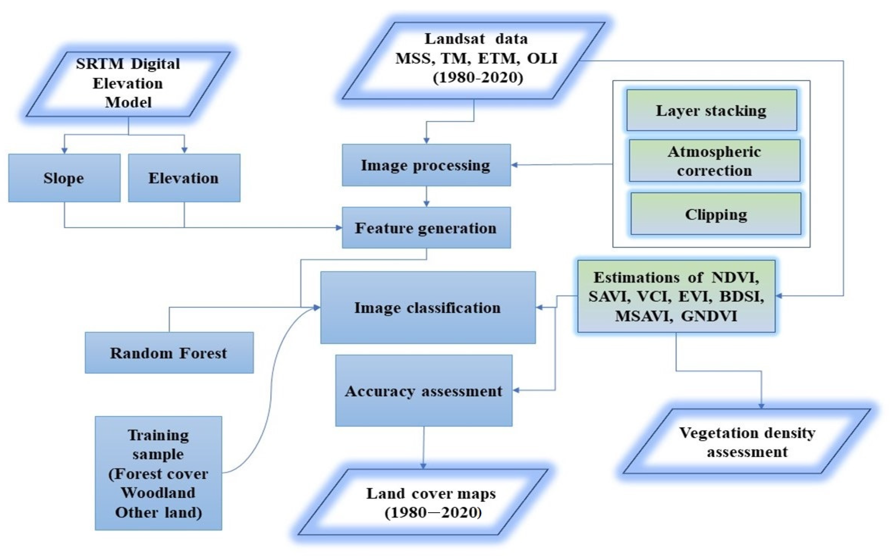
Figure 2 represents the stages of research. Pre- and post-processing techniques were applied to the Landsat images with ENVI and ArcGIS 10.5 software. The change in vegetation cover for each time was then estimated from each pixel. The categorization accuracy was assessed using statistical measures such as the kappa coefficient, user and producer error, and the statistical significance of overall accuracy. Forest cover and woodland cover changes for each of the time periods 1980, 1985, 1990, 2000, 2005, 2010, 2015, and 2020 were ascertained and evaluated.

2.3. Satellite Data Processing

The Landsat satellite series provides an excellent spatiotemporal resolution over recently launched satellites essential for assessing changes in plant cover over time. After the acquisition, data preprocessing improves the quality of satellite images before any interpretation or analysis can be carried out. Geometric distortion, haze reduction, cloud masking, and topographical and atmospheric corrections are among the corrections recommended for remote sensing data. Landsat data are routinely cleaned up by commercial data providers to remove systematic geometric distortion and radiometric inaccuracy. For retrieving and assessing significant information from remotely sensed data, Landsat image pre-processing is essential [37,38]. ENVI 4.7 software was used to pre-process satellite digital images in this study. Forest land cover seems to be more sensitive in the green, red, and near-infrared band for Landsat instruments including MSS, TM, ETM+, and OLI that were imported to ENVI 4.7 software for the pre-processing. Image calibration, geometrical correction, and atmospheric correction were all performed. Pan sharpening is the process of improving the spatial resolution of multispectral imagery by combining it with the higher resolution of a panchromatic band. There are several methods that can be used to accomplish this, as described in the literature [39]. The pan sharpening processes were performed for Landsat 7 and Landsat 8 images. Pan sharpening was only conducted on data acquired from sensors mounted on Landsat ETM and OLI. This is because the pan band is unavailable in Landsat 5 and earlier sensors of Landsat satellite. The entire study extent was covered in a single scene; therefore, mosaicking was not necessary. Layer stacking for the Landsat MSS, ETM+, or OLI bands was carried out in ENVI image processing software for the years 1980, 1985, 1990, 2000, 2005, 2010, 2015, and 2020, respectively. With a spatial resolution of 30 m, the images of the research region were projected to UTM zone 41 north [40]. In preparation for the computation of several indices and random forest classifier, each satellite image was processed.

2.4. Feature Generation

Vegetation indices for assessing vegetative covers have been developed and implemented by researchers during the past half century [41,42]. Spectral measurements are used as the basis for the generation of such indices [43]. This investigation made use of both spectral and temporal features in their respective forms. Landsat collection bands and features taken from raw and secondary data make up these features (e.g., DEM, slope, and aspect). Mention is made of specifics regarding features taken from the Landsat archive in an effort to improve the accuracy of the land use and land cover (LULC) classification. By using the vegetation index, we may gain an idea of how much greenery is present on the planet’s surface and how important it is for global climate change mitigation efforts. Consequently, the vegetation index is a helpful method for evaluating different types of vegetation cover in addition to forest cover.
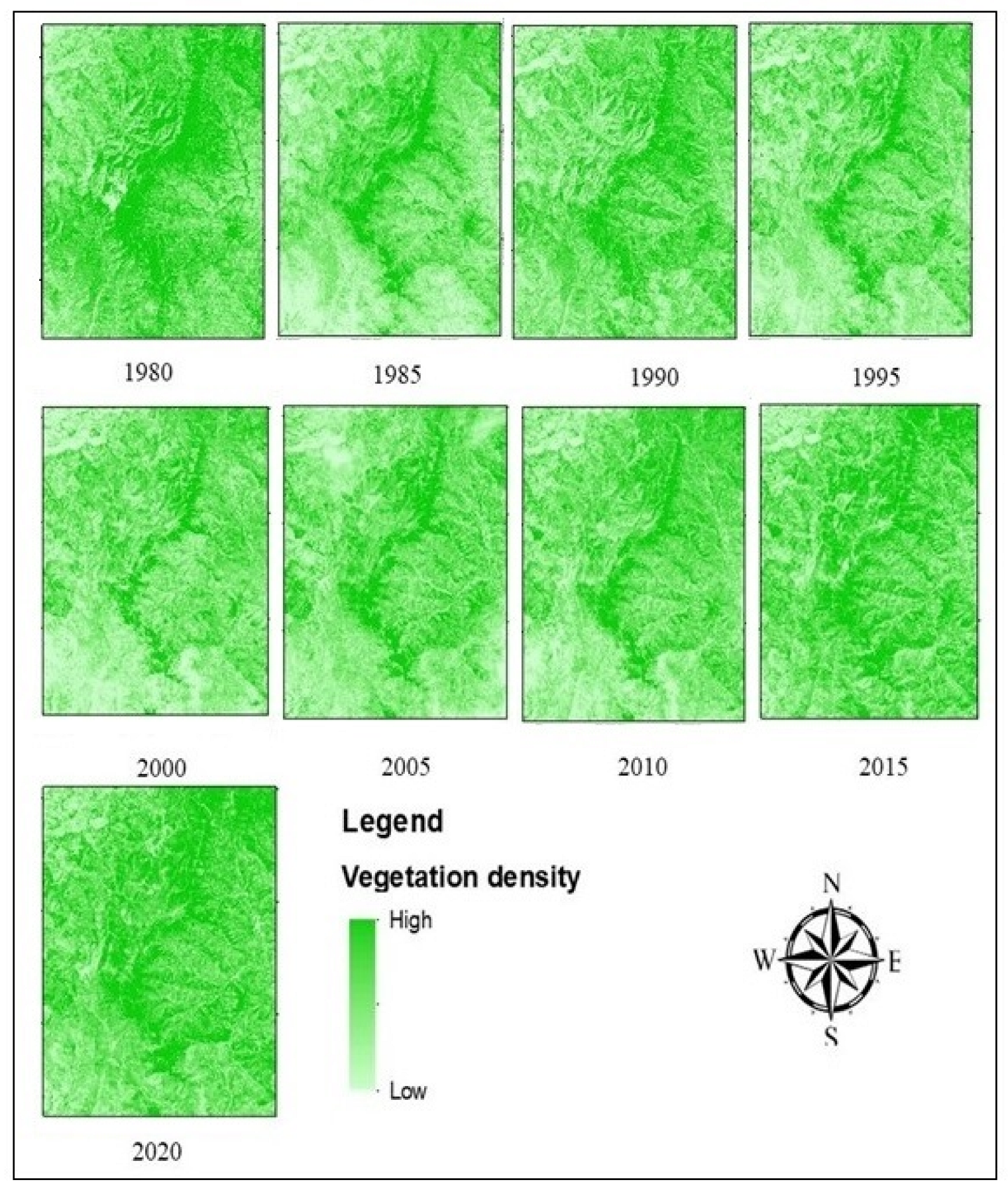
The NDVI’s maximum value indicates a forest, and its lowest value indicates little to no vegetation [44]. The values range from −1 to 1, where a negative number indicates an area that is devoid of vegetation or water bodies, and a positive value signifies the presence of vegetation. When the value of NDVI is high, it indicates the presence of a forest; when it is low, it reflects a lack of vegetation [45]. In 1998, Huete introduced the soil-adjusted vegetation index to limit the effect of soil background on the vegetation signal. He did this by introducing a constant soil adjustment factor L into the denominator of the NDVI model, where L changes based on the reflectance values of the soil. The soil-adjusted vegetation index (SAVI) was developed to reduce the influence of soil background on the vegetation signal. The vegetation condition proportion VCP is used in this study to indicate the levels of vegetation cover that are the highest, medium, and lowest over the course of the study periods. This is crucial for maximizing classification accuracy. In order to separate the NDVI’s short-term climate signal from its long-term ecological signal, a pixel-based normalization called the vegetation condition proportion (VCP) is used. It is more accurate than NDVI at assessing vegetation stress [46,47]. The vegetation was categorized as: high to very high, medium, and low to very low using the following vegetation indices: normalized difference vegetation index (NDVI), soil-adjusted vegetation index (SAVI), and vegetation cover proportion (VCP), respectively. Out of these, VCP gives more realistic results as shown in Figure 3. The greenness of vegetation can be measured with EVI, much like the normalized difference vegetation Index (NDVI). However, the enhanced vegetation index EVI is more sensitive in places with extensive vegetation and can account for some atmospheric conditions and canopy noise levels. An L value accounts for the canopy background, while C values are used as factors for the Earth’s atmospheric resistance, and blue band values are used to account for atmospheric conditions (B) [48]. Equations (1)–(3) were used for the estimation of shows NDVI, SAVI, and VCP. Barren land is indicated by higher dry built-up index (DBI) values, which can range from −2 to +2. When mapping areas of bare soil and areas with other types of vegetation, it is possible to use a suitable threshold for the non-vegetated class. A DBSI of 0.26 or higher was designated as soil surface for the research area, which depends on a test with a collection of soil pixels, while areas with lower values were classified as other classes. This was determined by a test with a collection of bare ground pixels [49]. Equations (4) and (5) were used for the estimation of DBI and EVI:
NDVI = (NR − R)/(NR + R)
SAVI = (NR − R) ∗ 1 + L/(NR + 1+L)
VCP = (NDVI − NDVImin)/(NDVImax − NDVImin)
DBI = (BLUE − TIR/BLUE + TIR) − NDVI
EVI = EVI = G ∗ ((NR − R)/(NR + C1 ∗ R − C2 ∗ B + L))
GNDVI = (NIR − GREEN)/(NDVI + GREEN)
where NR is near infrared, R is red band, and TIR is thermal infrared.

2.5. Image Classification Processing

It was determined that forests, woodland forests, and other types of land cover were included in the FAO’s 2015 classification system. However, we categorized the land cover as forest including open and closed forest. It does not include land that is used for agriculture or urban development in a major proportion. Woodland cover was considered vegetation (trees) cover that has a mean height of more than 5 m, with one or two tree species in the region, and the canopy cover is between 10% and 40% (scattered woody trees, shrubland, grassland, barren land, agricultural, and others). The study area land cover was divided into three primary categories: forest, woodland, and other land cover. Image classification is categorizing and labelling groups of pixels within an image. There are several approaches to image classification, including supervised, unsupervised, contextual, and hybrid methods. The effectiveness of these techniques depends on various factors, such as the complexity of the classes being classified, the amount of training data available, the number and type of input features, and the classifier method being used. Random forests (RF) are a popular solution for image classification tasks, as they often produce good results [50,51].

2.6. Random Forest Classification Processing

The random forest classifier is a machine-learning procedure focused on the ensemble learning method. Bierman was the one who first proposed this technique. In RF, various tree predictors are combined. The number of classification trees used, the number of variables used at each node, the random seed variable for decision tree construction, the minimum leaf population, the fraction of input variables that are bagged for each decision tree, and the out-of-bag mode are the six input parameters that are typically used by RF classifiers [52]. The overall classification accuracy rises with the rise in the number of trees. With replacement from the training data, each tree is parameterized using essentially a randomly selected collection of values. Assisting in the de-correlation of the trees reduces multicollinearity. This approach builds a training subset using random binary trees, above and beyond the clustering procedure. Additionally, the model is created from the primary database using a random sample of the training dataset. Using out-of-bag (OOB) outputs is one method for selecting optimum parameters [53]. Optimal parameter values are computed based on the RF method by analyzing the training data and testing it on the test data to ensure the best possible classification accuracy.
In order to better comprehend how various input features, such as Landsat image bands, many established vegetation and bare soil indices, and supplementary data, contribute to the final output, this study analyzed their relative values for extracting a land use and land cover (LULC) map. We accomplished this by using the RF classifier for the study area. In line with the suggestions of related studies [54], and the outcome to exclude the possibility of the OOB error in our data (Figure 4), we chose to focus on a sample size of 50 trees (ntree = 50). To determine which of these characteristics is most crucial, we used metrics such as the Gini index. Important variable characteristics are considered by RF algorithms through a mean decline in the Gini index (MDG). A characteristic with a higher frequency of occurrence across a larger number of nodes is more significant. At the node, the defined attribute is used to execute a splitting operation. In order to determine how many times each attribute was iterated until the RF algorithm’s classification was successful, the final count is taken once the classification is complete. Furthermore, the default value for the number of trials (mtry) was set to be the square root of the entire number of features. Based on Figure 4, the classifier appears to perform as well, with 50 and 100 trees to choose. The number of parameters per split that is specified by default was used, and the square root of the total number of variables was calculated. The default value was used for the minimum number of leaf populations. For all other random forest parameters, default values were used, including the fraction of input to bag per tree, the maximum number of leaf nodes, and the randomization seeds. Figure 3 indicates the significance of the RF tree number on classification accuracy.
Environmental issues such as disaster mitigation and management of water resources have been resolved using random forest (RF) methods. It can process a wide variety of data, including quantitative data and satellite images. The use of the RF classifier for LULC classification is shown to be extremely efficient in various studies of remote sensing applications [42,55]. This technique uses many trees to increase the precision of image classification and land use analysis [23,56,57]. The research community has become interested in it due to its remarkable classification outcomes and processing speed.

2.7. Accuracy Assessment

The most crucial final procedure in image classification is accuracy assessment [58,59]. Accuracy evaluation assists in providing a quantitative analysis of how efficiently and accurately pixels are allocated to the suitable land cover classes. Besides additional aspects, the level of resemblance between the generated and reference maps is described as accuracy. In recent years, a variety of strategies and indices for accuracy evaluation have been developed, and many of these have been enhanced. The overall accuracy and the kappa coefficient are the two frequently preferred accuracy indicators. Overall accuracy represents the probability of correctly classifying a randomly chosen area located on the maps. The kappa coefficient ranges from −1 to 1 and indicates that the classification is much accurate or worse [60,61]. A negative kappa value implies that the classification is significantly different from random. When the value is close to 1, it shows that the classification is more accurate [62,63]. The F1 measurement is currently widely used in most machine learning applications in binary situations and multiclass conditions. We also evaluated the suggested method’s performance using accuracy, precision, misclassification rate, recall, and specificity. The following formula is used to determine accuracy, misclassification rate, precision, recall, and specificity.
K   = OA   +   CA 1 CA  
F 1 = 2 Precision     recall Precision + recall  
Precision   =   Tp Tp   + Fn  
Recall   =   Tp Tp   + Fn    
Specificity =   Tn Tn   + Fp  
where OA represents the observed accuracy, and CA indicates the chance agreement. The metric for each class was calculated first, followed by the average score and between all categories, where Fn, Fp, Tp, and Tn, are the number of false-negative, false-positive, true-positive, and true-negative observations, respectively. First, the metric for each category was calculated, and then the average score across all categories was computed.

2.8. Training and Validation Data

This research focuses on an area that is dominated by three different types of LULC, all of which are described in Table 2 in full detail. Training and validation data were gathered through visual interpretation of high-resolution Google Earth images [64,65,66]. This procedure is widely used and documented in the scientific literature. The training and the validation samples were chosen sequentially for more accurate validation. Pixels were randomly divided into a training dataset of 70 percent and a validation dataset of 30 percent. Using the random point tool in ArcGIS 10.4, the same number of pixels were chosen at random for use in both the training and testing sets. These were spread out across the research area. Table 2 provides more explanation of the training and validation data depending on the extent and variability of the area that was taken into consideration in this research.

3. Results

The current research aimed to propose an effective approach for LULC identification. The proposed methodology is divided into four major parts. First, Landsat images were obtained, followed by training and testing data. After that, we introduced standard bands, as well as new classification variables. The images were then classified using the RF classification technique. Finally, we assessed the accuracy of the landcover map and its implications for the study area’s forest cover dynamics using test data. Figure 3 and Table 3 show that high to very-high vegetation density comprises areas with an altitude higher than 1700 m and medium-high vegetation density comprises about 44%, 22%, and 33% of the whole area from 1980, 2000, and 2020. Medium vegetation density was observed mostly from 1250–1700 m altitude in areas of 22%, 26%, and 18% for 1980, 2000, and 2020, while the majority of areas with low to very dense vegetation density cover are found at elevations of less than 1250 m. The percentage of land covered by low to very low vegetation was calculated to be 33 percent, 52 percent, and 49.2 percent in the year 1980, 2010, and 2020, respectively. Dense vegetation cover ranges from high in the northwest to medium in the south and from extremely low in the southeast to low in the southeast were observed, as demonstrated in Figure 3. Table 3 illustrates the distribution of vegetation cover from very high to high, medium to low, and low to very low vegetation cover and its variation and distribution with the digital elevation model.
We attempted to determine 8 features for the Landsat 1–3 time series data for the year 1980, and 33 features for the Landsat 4–5 time series data for the years 1985, 1990, and 1995. A total of 34 features were determined for the Landsat 7 image for the years 2000, 2005, and 2010. A total of 25 features for the Landsat 8 time series images for the years 2015 and 2020 were determined. In terms of the Landsat 5 images, B4, B5, DEM, and slope were the four variables that had the most significant impact. High-importance factors comprised DEM and B1 for the time series data obtained from Landsat 7, and B4, B11, and DEM for the time series data obtained from Landsat 8. However, to some extent, B3, DBI, and NDVI assisted in classifying all datasets. The overall outcomes indicate that DEM, B4, B5, B11, and VCP are the most critical factors for accurate RF classification, while GNDVI, EVI, and SAVI are less significant in the classification approach. The function plot (modelRF) was used to determine the optimal tree size (ntree) based on the OOB error rate. Inaccuracies in the OOB ranged from 0.021 to 0.0484. For all classes, OOB errors were exceptionally high between 22 trees. After 25 trees, the OOB errors remained constant. The OOB errors in the years 1980, 1990, and 2010 were the least, followed by 2005, 2015, and 2020 as shown in Figure 4. OOB errors were more prevalent in 1985 and 1995. The stability and saturation of the error and the time required to obtain the lowest error inform the decision of which ntree to use for the classification process. Time and computing process decreases as the number of decision trees decreases and vice versa, while there were some differences between the model parameters, which were not very distinguishable. As a result, we conducted extensive experiments across a wide range of values for the four variables including ntree, mtry, indices, and the spectral bands, to identify the optimal setup.

3.1. Land Cover Classification Analysis

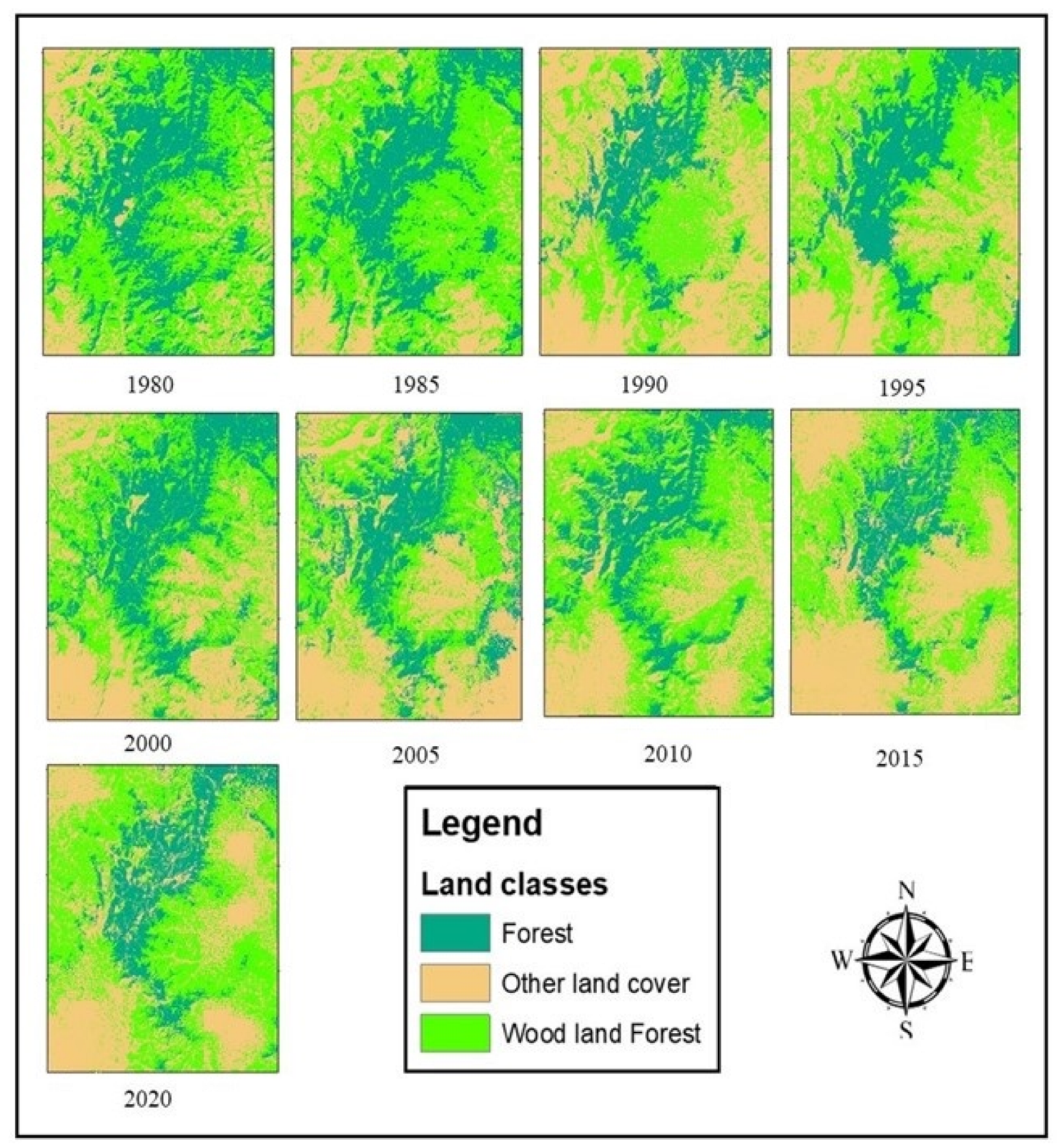
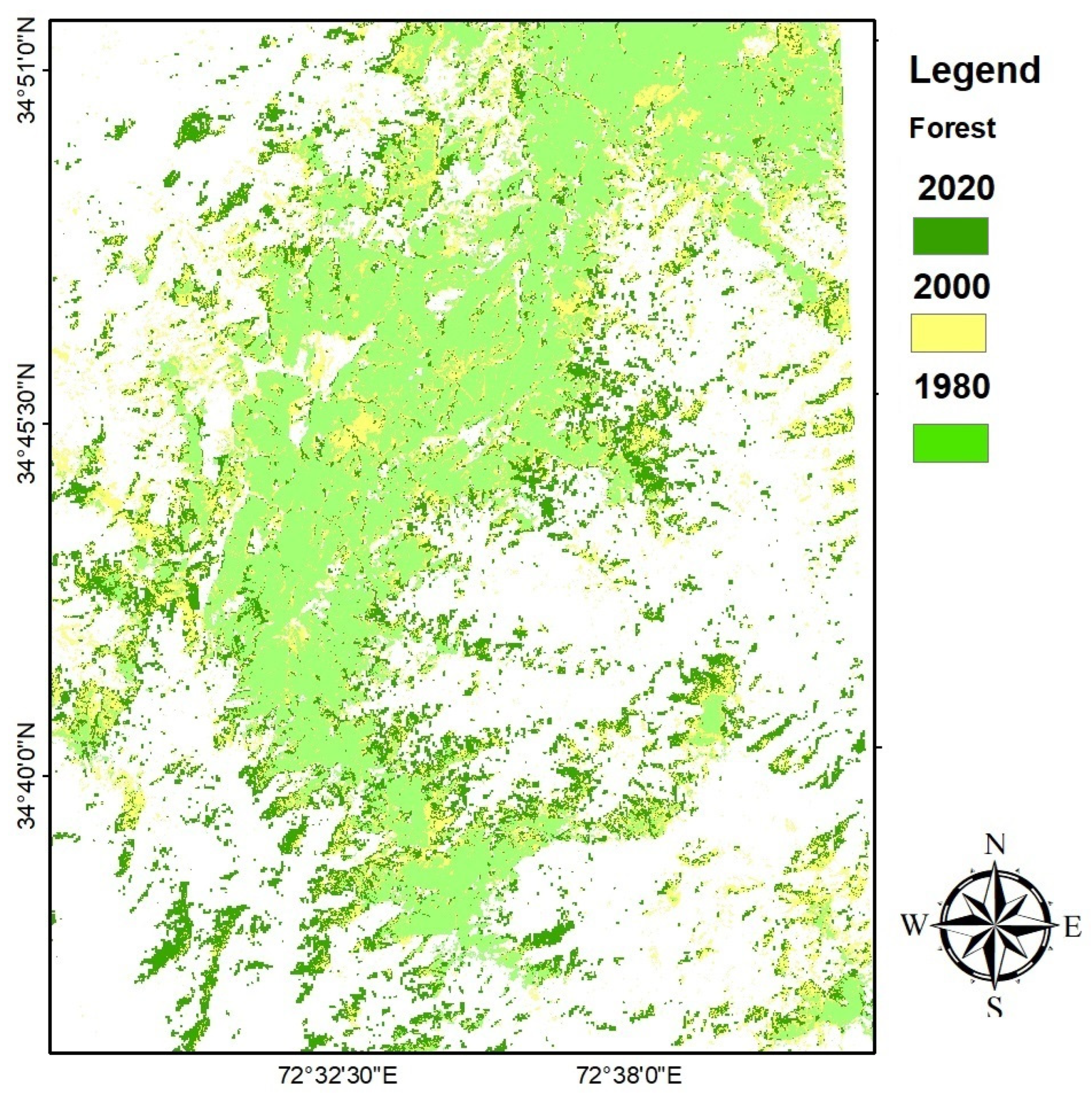
Forest, woodland, and other land cover types were identified and categorized throughout the research region using the random forest classification method. Because there is no body of water present, the research area was divided into the aforementioned three categories. Images captured by satellite in 1980, 1985, 1990, 2000, 2005, 2010, 2015 and 2020 were each assigned a category. About 84 km2 (35.3%) of total ever forest cover was lost in the past 40 years, and the highest rate of the total, approximately 34.71 km2, appeared between the 2000s and 2010. Results also show that recovery of forest cover was observed from 2015 to 2020 with a total of 16 km2. The forest and woodland cover decreased between 1980 and 2020, whereas other land covers increased for a total land area of 384.08 km2. Figure 5 shows the summary of each land cover change in km2 for the years 1980, 1985, 1990, 2000, 2005, 2010, 2015, and 2020. Figure 6 shows the RF classification results of the forest, woodland, and other lands in the study area for the years 1980, 1985, 1990, 2000, 2005, 2010, 2015, and 2020. Table 4 indicates the land cover statistics for three classes, including forest, woodland, and other land covers of Malam Jabba in square kilometers from 1980 to 2020.
Table 3 indicates that maximum forest cover estimated at an elevation of more than 1700 m occupied the northern western and central area of the Malam Jabba. There was a total of 236 km2 of forest cover in 1980 while in 2000 the loss reached 183 km2. However, an increase of 16 km2 in forest area was found from 2005 to 2020. The maximum loss of forest land was observed from 2000 to 2010, comprising 101 km2. It was also observed that the loss of forest land before 2000 was less compared with the period after 2000.
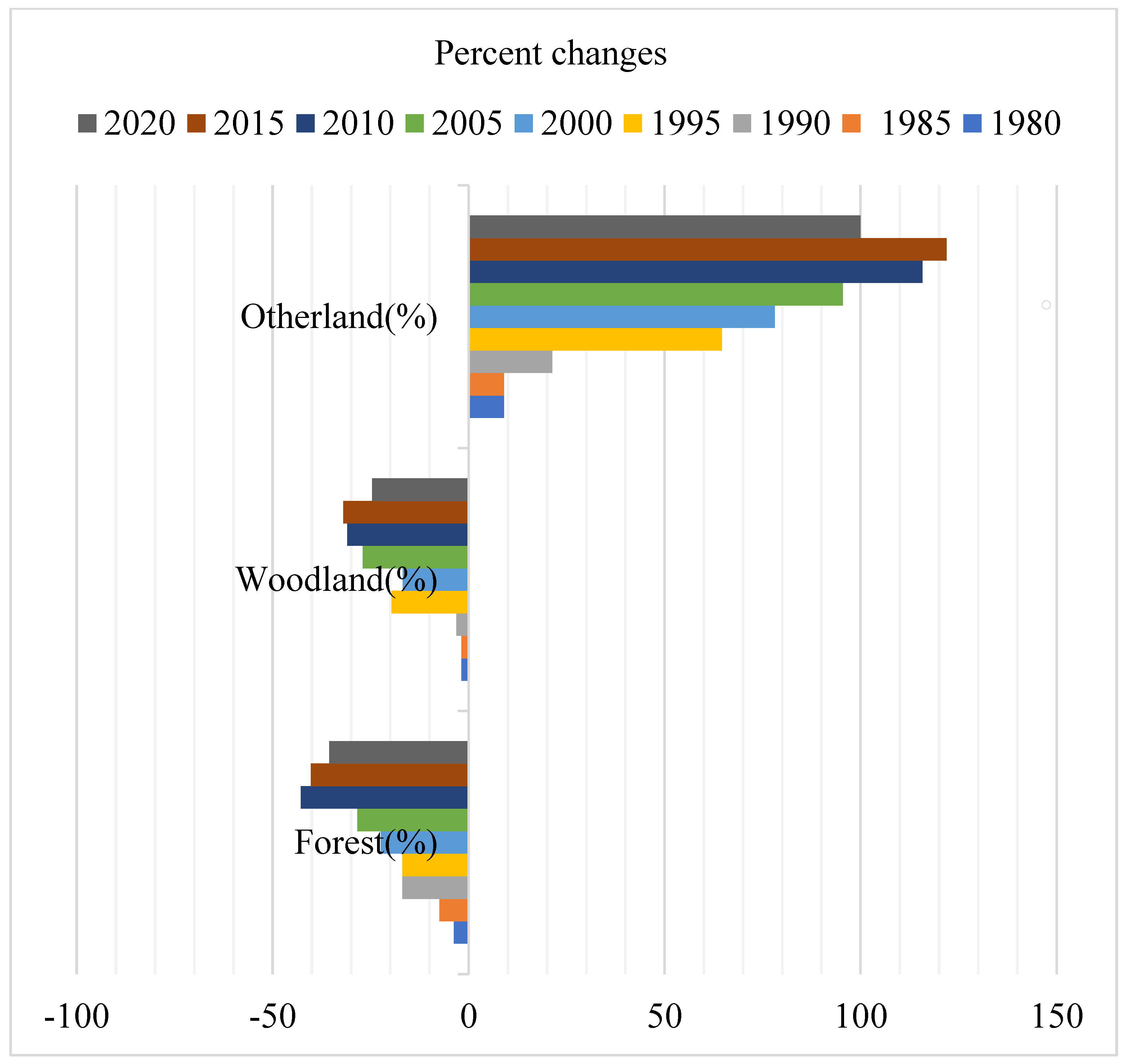
Forest land cover decreased during the research period from 1980 to 2020, as shown in Figure 6 and Figure 7, showing a drop of 32% km2. A total of 84 km declined in the area from 1980 to 2020. In every part of the country, the loss of forest cover posed a significant threat to the natural environment. Figure 5, Figure 6 and Figure 7 briefly explain the overall increase and decrease in three types of land cover maps that represent projections for the years 1980, 1985, 1990, 2000, 2005, 2010, 2015, and 2020. Table 3 explains the details of land cover change in square kilometers. The positive number shows the increase in land cover, while the negative number shows the area loss. Figure 6 shows the LULC map’s results for 9 years from 1980 through 2020 by using the RF classifier.
In Malam Jabba, the entire area covered by forests was around 235 km2 in 1990, which was reduced to 152 km2 by the year 2020, with a total forest cover loss of 35% percent. The minimum forest cover loss was observed from 2015 to 2020 with a value of 6%. The details of forest area lost in square kilometers within the gap of 5 years from 1980 to 2020 are indicated in Figure 8. Figure 9 explains the overlay analysis of forest cover change dynamics for a 20-year gap from 1980, 2000, and 2020.
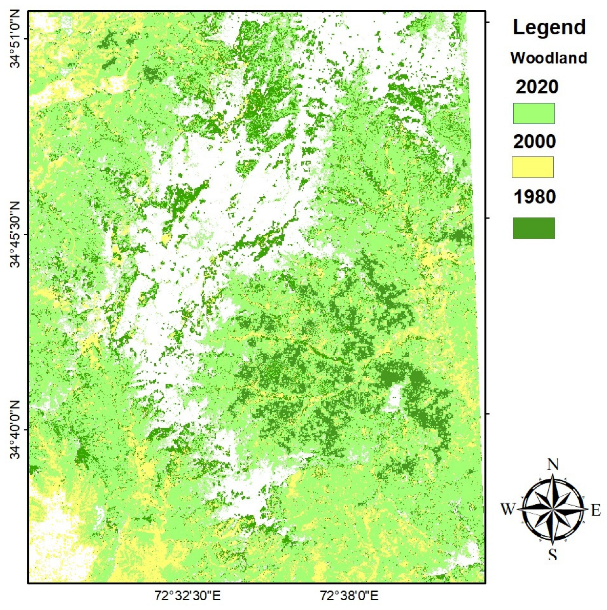
Woodland cover is primarily found between 1200 m and 1800 m in altitude throughout much of the spread around the study area’s northeastern and northwestern regions of the study area. The decline in woodland from 1980 to 2020 was observed at around 24%, with a decrease in the total area reaching 387 km2 from 281 km2. The reduction in woodland cover for 1990, 2000, 2010, and 2020 was 419 km2, 295 km2, 263 km2, and 287 km2. The total woodland cover lost in the past 40 years was about 94 km2. However, in later years a total of 24 km2 of woodland cover was recovered. Table 5 describes the details of the woodland area lost in square kilometers within the gap of 5 years from 1980 to 2020. Figure 9 represents the overlay analysis of woodland cover change dynamics between the 20-year gap of 1980, 2000, and 2020.
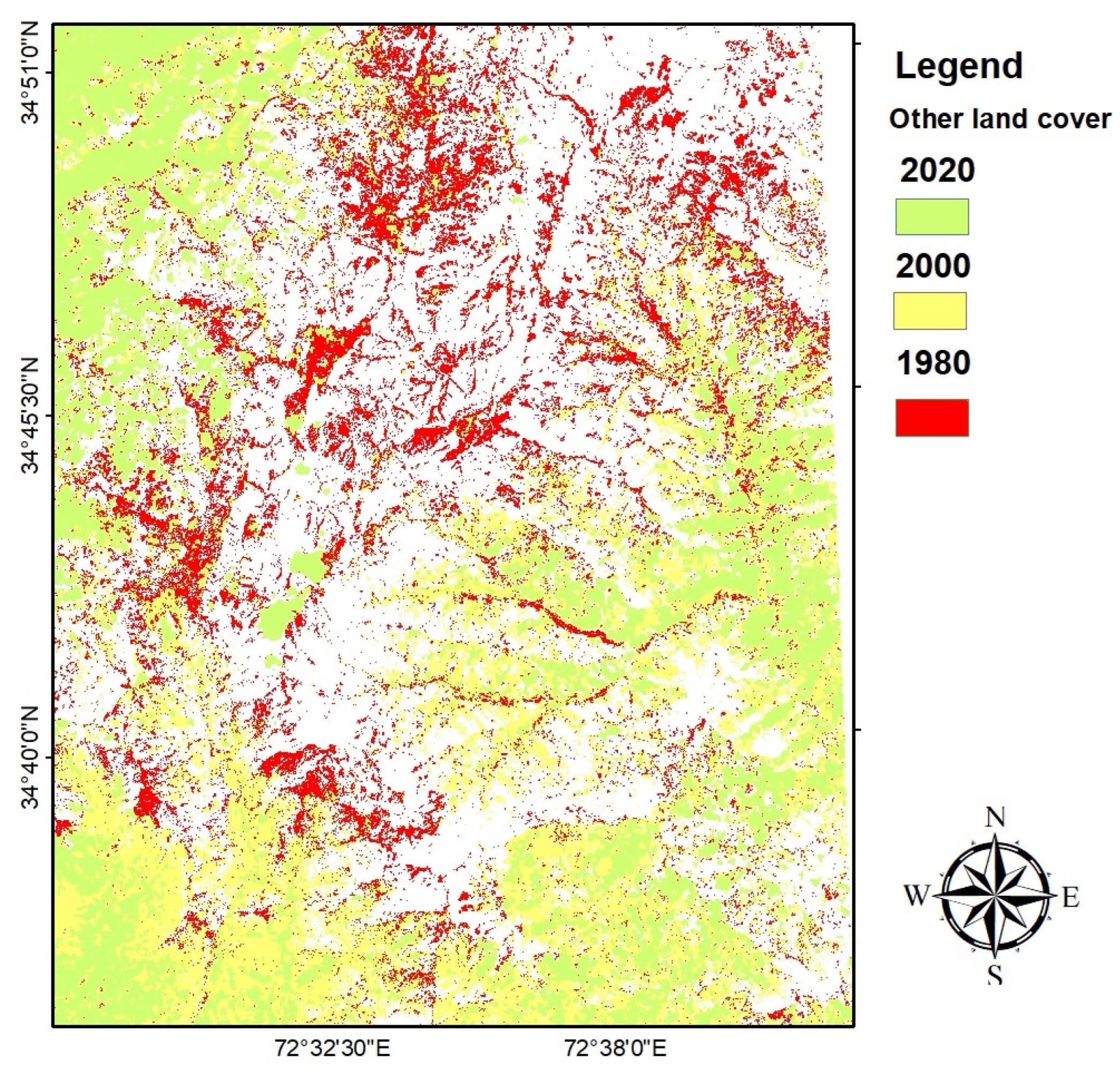
The remaining landmass is mainly comprised of low-altitude areas with an elevation of less than 1250 m. Between 1980 and 2020, the area covered by other land cover increased from 178.85 km2 to 356.23 km2, which is a 100 percent increase in the other land compared with other land cover classes, the maximum increase estimated during 2015 was 121% with a total area of 348 km2. The rise in woodland cover for the years 1985, 1995, 2005, and 2015 was 194 km2, 293 km2, 348 km2, and 395 km2. Over the past four decades, the total of other land cover has expanded by around 178 km2 at an average annual expansion rate of approximately 40 to 50 km2 in 2010. Figure 10 explains the details of other land cover areas lost in square kilometers between the 5 years from 1980 to 2020. Figure 10 represents the overlay analysis of other land cover change dynamics between the 20-year gap of 1980, 2000, and 2020. Most of the other land cover changes occurred in the western and southern directions of the study area, while a significant increase was observed toward the center of the study area.

3.2. Classification Accuracy Assessment

The accuracy assessment quantifies how well the pixels were sampled into appropriate land cover categories and is critical for analyzing and assessing remotely sensed data for land use/landcover change. Cross-tabulation, the confusion matrix, and the production of random samples were used to test classification accuracy [66,67]. Overall classification accuracies (OA) of at least 85% are considered desirable in remote sensing applications and land management [66,68]. For the 1980s, 2000s, and 2020, the statistical values of the overall accuracy, kappa coefficient, omission error (producer’s accuracy), and commission error (user’s accuracy) were calculated. According to the kappa statistics, which range from +1.0 to −1.0, the possibility of an agreement may be predicted to occur by chance. However, it varies from great agreement to weak agreement, correspondingly. Table 5 detail the 9 time periods from 1980 to 2020 with respect to producer and user accuracies, OA, kappa coefficients, accuracy, and F1-score. Table 5 shows that the OA and kappa for all datasets are pretty high, ranging from 0.90 to 0.96, respectively. The maximum overall accuracy of over 96% was obtained in 2000, followed by 2015 and 2020 compared with the other years. The forest cover and other land cover were most accurately classified compared with the woodland cover. The low UA and PA in the years 1980 and 1985 are responsible for these poor precisions. Classification statistics for LULC on 9 different periods from 1980 to 2020 are presented in Figure 7 and Table 6. The UA for forest and other land was approximately above 90%, while for the other land it was nearly 93%, and the PA for the forest was almost 92%. The model’s performance dropped dramatically for the woodland. Other lands obtained the maximum UA of over 95% in 2020 compared with the other classes, but its PA was only 90%. The UA and PA of the grassland were 68% and 90%, respectively. The least value of the F1 score, about 83%, was obtained forest in the year 1980, and the maximum values were 95% in the year 2020 compared with the other classes and years. Table 5 indicates the kappa statistics and overall accuracy, which is a measure of agreement or reliability. The estimated error matrix of sample counts is demonstrated, along with the user’s accuracy, the producer’s accuracy, and the F1-score.

4. Discussion

Land cover change classification assessment and analysis from remotely sensed images has been the most helpful method since the availability of satellite images in the 1970s, when they became more advanced and improved in reliability and accuracy due to continuous advancements in remote sensing technology. Very few studies and research were conducted using high-resolution airborne or space remote sensing data in the Malam Jabba region for land use classification, especially when evaluating changes in land cover and its impact on evergreen forest. In this study, forest and woodland changes for the 1980s were retrieved and evaluated. As a result, using the random forest method of classification for forest, woodland, and other land cover change was retrieved with excellent accuracy, as discussed in the paper. In this research we used different spectral indices and other data. These findings helped classify land use in the research area from 1980 to 2000, and 9 suggested classification periods enabled land cover classification. LULC data have been extracted from Sentinel-2 data recently. Sentinel-2 data have a high spatial resolution, but Landsat has monitored Earth for over 50 years, making it a preferred source for LULC change research. The relative importance of the spectral bands and the vegetative indices in classification accuracy were critical parameters investigated in this work. Using vegetation indices can improve the classification of forest areas and other land types in land cover classification studies [68,69,70,71]. The NDVI’s significance as a vegetation approximation was to be expected. As the SAVI adjusts for soil reflectance on vegetation reflectance, it is advantageous in sparsely vegetated places [72,73]. Hence its relatively high importance was to be expected. It is quite remarkable that the GNDVI, which was designed to improve sensitivity to thick forests, has such a large impact [74,75]. Following this, it was anticipated that vegetation indices would provide further support to the classification results. Overall, from the beginning of the 1980s to the end of 2022, there was a considerable amount of forest loss. About 26 km2, 53 km2, 101 km2, and 84 km2 of forest cover were lost in 1990, 2000, 2010, and 2020, respectively, and the maximum loss of forest cover happened between 2000 and 2010. Woodland cover decreased by about −3.1%, −16.7%, −30%, and −24% in 1990, 2000, 2010, and 2020. The maximum decline in wood cover happened between 2000 to 2010. Figure 5 shows the total forest cover change in 1980s, 2000s, and 2020s based on our study as according to the statistical value of the country’s total forest estimated by the FAO. According to past studies in the region of interest, the current temporal forest cover analysis in the Swat district area for the years 1968, 1990, and 2007 reveals a yearly rate of deforestation of 1.86%, 1.28%, and 0.80% including the scrub forest, agro-forest, and alpine forest regions, consecutively [76]. The Swat and Shangla regions experienced an average yearly gross deforestation rate of 0.81% between 2001 and 2009. Moreover, between 1996 and 2008, the Hazara as well as the Malakand regions had an annual forest cover rate of change of 1.32%. Schickhoff reports that long-term analyses show a 50 percent decline in forested land in the Kaghan and Naran Valley of Khyber Pakhtunkhwa province between 1847 and 1990 [77].
This research’s findings are consistent with those of others that have showed increased yearly rate of deforestation in a number of developing countries. FAO analyses (2005) indicate a 23.3% loss in the forest land of Pakistan from 1990 to 2005, further supporting the findings for a faster rate of deforestation. The Environment Assessment Programme for the Asia–Pacific region found that between 1981 and 1990 there was an annual drop of 0.6%. (UNEP and ICIMOD, 1998, pp. 29–31). In a similar vein, Brown and Durst (2003) estimated that the annual rate of deforestation in the United States during the 1990s was 1.5%. In Africa, Brink and Eva found in 2009 that agricultural land had grown from around 200 million hectares to 340 million hectares over a 25-year period. This expansion was due to a loss of forest cover, which decreased by 16% [12,78]. According to Wyman and Stein, from 1989 to 2004 Belize lost 30% of its forest cover, with deforestation being more prevalent in regions close to roads in 2010 [79]. From 1963 until 1993, Semwal found a 30% increase in crop land in the central Himalaya region in India at the cost of a 5% decrease in forest. Keleş, Sivrikaya, akir, and Köse in 2008 observed an annual decrease of 0.42 percent of forest cover in Trabzon, Turkey, between 1975 and 2000 [56,80]. Around the Changbai Biosphere Reserve in China, Zheng, Wallin, and Hoa (1997) found an average rate of forest loss of 1.12%.
Integrating time-varying remote sensing data into auxiliary datasets increases the variety of spectral signatures used to train the model; therefore, this finding makes sense. A model’s capacity to accurately categorize picture pixels that differ from the most prevalent spectral signatures of the classifications improves in proportion to the amount of variation included in the training data. This confirms the importance of integrating spatiotemporal datasets of satellite remote sensing image classification, as demonstrated in prior studies. [81,82,83].
Even though it is hard to ascertain the classification performance with reality or with the actual features on the ground, constructing matrix errors may reduce the classification errors that could result from the clustering of spectral pixel values during the classification process. This is despite the fact that it is impossible to compare the accuracy of classification with reality [84,85]. One of the most popular techniques in assessing classification accuracy is the confusion matrix; however, it may not always reflect reality because accuracy can be influenced by a variety of factors, such as availability of very high-resolution datasets. Additionally, the accuracy may be impacted by the shadows of mountain slopes, where the topography is quite rocky and mountainous. According to this study’s findings, forest loss was mostly a result of human activity and was particularly severe along roads, rivers, and at the top and bottom of several ridges. Climate change-related factors such as drought, insufficient precipitation, or flood, on the other hand, can exacerbate forest loss. The forest land was seriously harmed by the market sale of live trees during droughts, particularly the drought between 1999 and 2001. However, the government has implemented a conservation strategy that involves afforestation and reforestation. The area of forest may be restored and the annual rate of forest cover loss might be reduced as a result. Deforestation in the district is frequently brought on by human activity, such as clearing land for traditional farming practices, lumber, fuel wood, and traditional homes, especially during the 1980s and 2000 [86,87]. The largest rate of deforestation occurs in KP province, which is tied to rising demand for firewood from a growing population and is exacerbated by widespread unauthorized commercial woodcutting. Small-scale tree cutting as a source of income may be a testimony to the current timber demand scenario, which is characterized by a drop in agricultural regions and a decrease in population territories [88,89]. Moreover, this position has been exacerbated by recent security battles along the western frontiers. The clearing by security troops for tactical reasons and the financial profits of the timer mafia have both been linked to deforestation [90,91]. However, some studies have found much higher rates of deforestation as a result of industrial-scale logging, irregular agricultural development, and fuel wood collecting in economically depressed remote regions [4,63]. Effective policy is key to addressing the issue of deforestation and promoting sustainable forest management. Some policy measures that can contribute to this goal include: developing and enforcing clear regulations and laws prohibiting illegal logging and other activities contributing to deforestation, which can include measures such as strengthening penalties for violators and creating mechanisms for monitoring and enforcing compliance; promoting land use planning and zoning that considers the environmental and social impacts of different land uses, which can help ensure that forests are protected and that development sustainably takes place and respects the rights of local communities; and encouraging sustainable forestry practices, such as selective logging and reforestation, through incentives and education programs, which can help ensure that forests are managed in a way that preserves their ecological value and supports local communities livelihoods.
This study can contribute to the literature on sustainability and deforestation issues by providing a detailed analysis of forest and other vegetation cover assessments using satellite remote sensing to implement a specific context and its impact on forest management. By examining the successes and challenges of these measures, the study can provide valuable insights and lessons for policymakers and other stakeholders working to address these issues. Additionally, the analysis can highlight the importance of considering the perspectives and needs of local communities in the development and implementation of policy, as well as the role that stakeholder engagement can play in promoting sustainable forest management.

Limitations of the Study

Limitations of the study include that the satellite data may not accurately map forests, especially in areas with complex topography or dense canopy cover. In these cases, ground-based data may be needed to supplement the satellite data and improve the accuracy of the forest map. Second, satellite data may be subject to spatial resolution limitations, which can affect the accuracy of the forest map. For example, data with low spatial resolution may not provide sufficient detail to map small-scale features such as individual trees accurately. Third, the accuracy of the forest map may be affected by the quality and availability of ancillary data, such as digital elevation models and land cover maps, which are often used to improve the accuracy of the forest map. Finally, the analysis results may be limited by the sample size and the representativeness of the case study area. A larger sample size and a more diverse range of case study areas may provide more robust and generalizable results. The random forest method is a relatively complex algorithm that can be difficult to understand and interpret for some users. This can make it challenging to explain the results of a random forest model to non-technical stakeholders. The model’s output may be unreliable if the input data are incomplete, noisy, or biased. Overfitting is another limitation of this study. The random forest can be prone to overfitting, which occurs when a model is too closely tailored to the training data and does not generalize well to new data. This can lead to poor performance on unseen data.

5. Conclusions

The study shows that the loss of forest land is a serious environmental issue in the northern area of Pakistan. This research has shed light on how the vegetation cover has changed in the Malam Jabba region during the past forty years. The different categories are high to very high, medium, and low to extremely low vegetation cover. Based on the background, random forest appeared to be a promising technique for mapping LULC from satellite imagery. Three distinct LULC classes, including forest, woodland forest, and other land cover, were mapped from Landsat MMS, TM, ETM+, and OLI images using the random forest classifier in this research. To optimize the RF settings, we used methods based on the out-of-bag (OOB) estimate of error while also considering the impact of each of Landsat’s spectral bands. We tested a range of tree numbers and RF input settings and found 50 trees to be optimal. Malam Jabba’s total forest land area in 1980 was roughly 236 km2, which shrank by 154 km2 in 2020, and the overall rate of forest cover loss was 32 percent. Woodland cover loss from 1980 to 2020 was 18 km2, or around 27.43 percent, with a 2.1 km2/yr annual deforestation rate. The overall accuracy, kappa values, and F1-score were all between 91 to 96%, while kappa was 0.90 to 0.96 and the F1-score was 0.87 to 0.93 between 1980 to 2020, respectively. Policymakers must develop effective strategies to reduce these changes in how land is used. The remaining forest will be lost if no action is taken to stop the rapid pace of deforestation that is currently occurring. The FAO’s statistics on forest cover, which show that the loss of forest is very high and significant, are consistent with the conclusion, even though the annual rate of deforestation figure differs from other estimates. The main causes of deforestation in the nation are anthropogenic activities including overgrazing, urbanization, road construction, firewood collection, and subsistence farming. This is a matter of fact; if proper management, planning, and strategies are not put into place to improve and maintain the high rate of deforestation currently present, then any remaining forests will not be sustained for a longer period of time and this will negatively affect the socioeconomic situation of the area.

Author Contributions

Conceptualization, A.I. and S.Z.; Methodology, M.J. and M.S.; Software, M.S.; Validation, M.J. and M.S.; Formal analysis, M.J. and A.K.; Investigation, M.J.; Resources, M.J., M.S. and S.Z.; Data curation, A.I. and A.K.; Writing—original draft, M.J. and M.S.; Writing—review & editing, M.J. and M.S.; Visualization, M.S.; Supervision, J.S.; Project administration, M.J.; Funding acquisition, J.S. All authors have read and agreed to the published version of the manuscript.

Funding

This research was funded by the science and technology plan of Gansu Province. Research on Key Technologies of automatic monitoring of surface cover change in Gansu Province (20yf3ga013).

Institutional Review Board Statement

Not applicable.

Informed Consent Statement

Not applicable.

Data Availability Statement

Not applicable.

Conflicts of Interest

The authors declare no conflict of interest.

References

  1. Mahmoud, S.H.; Gan, T.Y. Impact of anthropogenic climate change and human activities on environment and ecosystem services in arid regions. Sci. Total Environ. 2018, 633, 1329–1344. [Google Scholar] [CrossRef] [PubMed]
  2. Bonan, G.B. Forests and climate change: Forcings, feedbacks, and the climate benefits of forests. Science 2008, 320, 1444–1449. [Google Scholar] [CrossRef] [PubMed] [Green Version]
  3. Gebrehiwot, S.G.; Bewket, W.; Gärdenäs, A.I.; Bishop, K. Forest cover change over four decades in the Blue Nile Basin, Ethiopia: Comparison of three watersheds. Reg. Environ. Chang. 2014, 14, 253–266. [Google Scholar] [CrossRef]
  4. Qamer, F.M.; Abbas, S.; Saleem, R.; Shehzad, K.; Ali, H.; Gilani, H. Forest Cover Change Assessment in Conflict-Affected Areas of Northwest Pakistan: The Case of Swat and Shangla Districts. J. Mt. Sci. 2012, 9, 297–306. [Google Scholar] [CrossRef]
  5. Marland, G.; Pielke, R.A., Sr.; Apps, M.; Avissar, R.; Betts, R.A.; Davis, K.J.; Frumhoff, P.C.; Jackson, S.T.; Joyce, L.A.; Kauppi, P.; et al. The climatic impacts of land surface change and carbon management, and the implications for climate-change mitigation policy. Clim. Policy 2003, 3, 149–157. [Google Scholar] [CrossRef] [Green Version]
  6. Keenan, R.J.; Reams, G.A.; Achard, F.; de Freitas, J.V.; Grainger, A.; Lindquist, E. Dynamics of global forest area: Results from the FAO Global Forest Resources Assessment 2015. For. Ecol. Manag. 2015, 352, 9–20. [Google Scholar] [CrossRef]
  7. FAO. FRA 2015, Terms and Definitions. Forest Resources Assessment, Working Paper 180. Food and Agriculture Organization of the United Nations. 2012, Volume 36. Available online: www.fao.org/forestry/fra (accessed on 4 October 2022).
  8. Anon. 352 Forest Ecology and Management Global Forest Resources Assessment 2015. Available online: http://www.fao.org/forestry/fra2005/en/ (accessed on 6 October 2022).
  9. Morales-Barquero, L.; Skutsch, M.; Jardel-Peláez, E.J.; Ghilardi, A.; Kleinn, C.; Healey, J.R. Operationalizing the Definition of Forest Degradation for REDD+, with Application to Mexico. Forests 2014, 5, 1653–1681. [Google Scholar] [CrossRef] [Green Version]
  10. MacDicken, K.G. Global Forest Resources Assessment 2015: What, Why and How? For. Ecol. Manag. 2015, 352, 3–8. [Google Scholar] [CrossRef] [Green Version]
  11. Qamer, F.M.; Shehzad, K.; Abbas, S.; Murthy, M.S.R.; Xi, C.; Gilani, H.; Bajracharya, B. Mapping deforestation and forest degradation patterns in Western Himalaya, Pakistan. Remote Sens. 2016, 8, 385. [Google Scholar] [CrossRef] [Green Version]
  12. Brink, A.B.; Eva, H.D. Monitoring 25 years of land cover change dynamics in Africa: A sample based remote sensing approach. Appl. Geogr. 2009, 29, 501–512. [Google Scholar] [CrossRef]
  13. Bouslihim, Y.; Kharrou, M.H.; Miftah, A.; Attou, T.; Bouchaou, L.; Chehbouni, A. Comparing Pan-sharpened Landsat-9 and Sentinel-2 for Land-Use Classification Using Machine Learning Classifiers. J. Geovisualization Spat. Anal. 2022, 6, 35. [Google Scholar] [CrossRef]
  14. Reddy, C.; Sudhakar, C.; Jha, S.; Dadhwal, V.K. Assessment and Monitoring of Long-Term Forest Cover Changes in Odisha, India Using Remote Sensing and GIS. Environ. Monit. Assess. 2013, 185, 4399–4415. [Google Scholar] [CrossRef] [PubMed]
  15. Sohail, M.; Ali, S.S.F.; Fatima, E.; Nawaz, D.A. Spatio-temporal analysis of land use dynamics and its potential implications on land surface temperature in lahore district, punjab, pakistan. Int. Arch. Photogramm. Remote Sens. Spatial Inf. Sci. 2021, XLIII-B3-2021, 359–367. [Google Scholar] [CrossRef]
  16. Otukei, J.R.; Blaschke, T. Land cover change assessment using decision trees, support vector machines and maximum likelihoodclassification algorithms. Int. J. Appl. Earth Obs. Geoinf. 2010, 12, S27–S31. [Google Scholar]
  17. Alzubaidi, L.; Zhang, J.; Humaidi, A.J.; Al-Dujaili, A.; Duan, Y.; Al-Shamma, O.; Santamaría, J.; Fadhel, M.A.; Al-Amidie, M.; Farhan, L. Review of deep learning: Concepts, CNN architectures, challenges, applications, future directions. J. Big Data 2021, 8, 1–74. [Google Scholar]
  18. Naushad, R.; Kaur, T.; Ghaderpour, E. Deep Transfer Learning for Land Use and Land Cover Classification: A Comparative Study. Sensors 2021, 21, 8083. [Google Scholar] [CrossRef]
  19. Pires de Lima, R.; Marfurt, K. Convolutional neural network for remote-sensing scene classification: Transfer learning analysis. Remote Sens. 2019, 12, 86. [Google Scholar] [CrossRef] [Green Version]
  20. Badhe, A.; Chang, S. Fast image classification by boosting fuzzy classifier. Neural Netw. Mach. Learn. 2016, 327, 175–182. [Google Scholar]
  21. Kamavisdar, P.; Saluja, S.; Agrawal, S. A survey on image classification approaches and techniques. Int. J. Adv. Res. Comput. Commun. Eng. 2013, 2, 1005–1009. [Google Scholar]
  22. Thanh Noi, P.; Kappas, M. Comparison of Random Forest, k-Nearest Neighbor, and Support Vector Machine Classifiers for LandCover Classification Using Sentinel-2 Imagery. Sensors 2018, 18, 18. [Google Scholar] [CrossRef] [Green Version]
  23. Tassi, A.; Gigante, D.; Modica, G.; Di Martino, L.; Vizzari, M. Pixel-vs. Object-Based Landsat 8 Data Classification in Google EarthEngine Using Random Forest: The Case Study of Maiella National Park. Remote Sens. 2021, 13, 2299. [Google Scholar] [CrossRef]
  24. Wang, C.; Shu, Q.; Wang, X.; Guo, B.; Liu, P.; Li, Q. A random forest classifier based on pixel comparison features for urban LiDAR data. ISPRS J. Photogramm. Remote Sens. 2019, 148, 75–86. [Google Scholar] [CrossRef]
  25. Belgiu, M.; Drăguţ, L. Random forest in remote sensing: A review of applications and future directions. ISPRS J. Photogramm. Remote Sens. 2016, 114, 24–31. [Google Scholar] [CrossRef]
  26. Chapman, D.S. Random Forest Characterization of Upland Vegetation and Management Burning from Aerial Imagery. J. Biogeogr. 2010, 37, 37–46. [Google Scholar] [CrossRef]
  27. Sesnie, S.E.; Gessler, P.; Finegan, B.; Thessler, S. Integrating Landsat TM and SRTM-DEM Derived Variables with Decision Trees for Habitat Classification and Change Detection in Complex Neotropical Environments. Remote Sens. Environ. 2008, 112, 2145–2159. [Google Scholar] [CrossRef]
  28. Van Beijma, S.; Comber, A.; Lamb, A. Random forest classification of salt marsh vegetation habitats using quad-polarimetric airborne SAR, elevation and optical RS data. Remote Sens. Environ. 2014, 149, 118–129. [Google Scholar] [CrossRef]
  29. Saeys, Y.; Inza, I.; Larrañaga, P. A review of feature selection techniques in bioinformatics. Bioinformatics 2007, 23, 2507–2517. [Google Scholar] [CrossRef] [Green Version]
  30. Baumann, M.; Ozdogan, M.; Wolter, P.T.; Krylov, A.; Vladimirova, N.; Radeloff, V.C. Landsat remote sensing of forest windfall disturbance. Remote Sens. Environ. 2014, 143, 171–179. [Google Scholar] [CrossRef]
  31. Chasmer, L.; Hopkinson, C.; Veness, T.; Quinton, W.; Baltzer, J. A decision-tree classification for low-lying complex land cover types within the zone of discontinuous permafrost. Remote Sens. Environ. 2014, 143, 73–84. [Google Scholar] [CrossRef]
  32. Dronova, I.; Gong, P.; Wang, L.; Zhong, L. Mapping dynamic cover types in a large seasonally flooded wetland using extended principal component analysis and object-based classification. Remote Sens. Environ. 2015, 158, 193–206. [Google Scholar] [CrossRef]
  33. Sohail, M.; Ali, S.S.F. Abidullah: Monitoring Vegetation Density Using Spectral Vegetation Indices: A Case Study of Malam Jabba Region, District Swat, Pakistan. Int. Arch. Photogramm. Remote Sens. Spatial Inf. Sci. 2022, XLVI-M-2-2022, 185–190. [Google Scholar] [CrossRef]
  34. Silleos, N.G.; Alexandridis, T.K.; Gitas, I.Z.; Perakis, K. Vegetation Indices: Advances Made in Biomass Estimation and Vegetation Monitoring in the Last 30 Years. Geocarto Int. 2006, 21, 21–28. [Google Scholar] [CrossRef]
  35. Diaz-Uriarte, R.; Alvarez de Andres, S. Gene selection and classification of microarray data using random forest. BMC Bioinform. 2006, 7, 3. [Google Scholar] [CrossRef] [PubMed] [Green Version]
  36. Lund, H. Gyde. Definitions of Forest, Deforestation, Afforestation, and Reforestation. Gainesville, VA: Forest Information Services. Misc. pagination. 2015, Volume 14. Available online: https://www.researchgate.net/publication/259821294_Definitions_of_Forest_Deforestation_Afforestation_and_Reforestation (accessed on 2 October 2022).
  37. Butt, A.; Shabbir, R.; Ahmad, S.S.; Aziz, N. Land use change mapping and analysis using Remote Sensing and GIS: A case study of Simly watershed, Islamabad, Pakistan. Egypt. J. Remote. Sens. Space Sci. 2015, 18, 251–259. [Google Scholar] [CrossRef]
  38. Iqbal, M.F.; Khan, I.A. Spatiotemporal land use land coverchange analysis and erosion risk mapping of Azad Jammu and Kashmir, Pakistan. Egypt. J. Remote Sens. Space Sci. 2014, 17, 209–229. [Google Scholar]
  39. Bwangoy, J.R.; Hansen, M.C.; Roy, D.P.; De Grandi, G.; Justice, C.O. Wetland mapping in the Congo Basin using optical and radar remotely sensed data and derived topographical indices. Remote Sens. Environ. 2010, 114, 73–86. [Google Scholar] [CrossRef]
  40. Petta, R.A.; Carvalho, L.V.; Erasmi, S.; Jones, C. Evaluation of desertification processes in serido region (NE Brazil). Int. J. Geosci. 2013, 4, 12–17. [Google Scholar] [CrossRef] [Green Version]
  41. Karathanassi, V.; Kolokousis, P.; Ioannidou, S. A comparison study on fusion methods using evaluation indicators. Int. J. Remote Sens. 2007, 28, 2309–2341. [Google Scholar] [CrossRef]
  42. Khelifi, L.; Mignotte, M. Deep Learning for Change Detection in Remote Sensing Images: Comprehensive Review and Meta-Analysis. IEEE Access 2020, 8, 126385–126400. [Google Scholar] [CrossRef]
  43. Bhatti, S.S.; Tripathi, N.K. Built-up area extraction using Landsat 8 OLI imagery. GIScience Remote Sens. 2014, 51, 445–467. [Google Scholar] [CrossRef] [Green Version]
  44. Jeevalakshmi, D.; Reddy, S.N.; Manikiam, B. Land cover classification based on NDVI using LANDSAT8 time series: A case study Tirupati region. In Proceedings of the 2016 International Conference on Communication and Signal Processing (ICCSP), Melmaruvathur, India, 6–8 April 2016; pp. 1332–1335. [Google Scholar]
  45. Liu, H.Q.; Huete, A. A feedback-based modification of the NDVI to minimize canopy background and atmospheric noise. IEEE Trans. Geosci. Remote Sens. 1995, 33, 457–465. [Google Scholar] [CrossRef]
  46. Li, P.; Jiang, L.; Feng, Z. Cross-comparison of vegetationindices derived from Landsat-7 Enhanced Thematic Mapper Plus(ETM+) and Landsat-8 operational land imager (OLI) Sensors. Remote Sens. 2014, 6, 310–329. [Google Scholar] [CrossRef] [Green Version]
  47. Zhang, X.; Delu, P.; Chen, J.; Zhan, Y.; Mao, Z. Using longtime series of Landsat data to monitor impervious surface dynamics a case study in the Zhoushan Islands. J. Appl. Remote Sens. 2013, 7, 073515. [Google Scholar] [CrossRef] [Green Version]
  48. Huete, A.; Didan, K.; Miura, T.; Rodriguez, E.; Gao, X.; Ferreira, L. Overview of the radiometric and biophysical performance of the MODIS vegetation indices. Remote Sens. Environ. 2002, 83, 195–213. [Google Scholar] [CrossRef]
  49. Rasul, A.; Balzter, H.; Ibrahim, G.R.F.; Hameed, H.M.; Wheeler, J.; Adamu, B.; Ibrahim, S.; Najmaddin, P.M. Applying Built-Up and Bare-Soil Indices from Landsat 8 to Cities in Dry Climates. Land 2018, 7, 81. [Google Scholar] [CrossRef]
  50. Madanian, M.; Soffianian, A.R.; Koupai, S.S.; Pourmanafi, S.; Momeni, M. Analyzing the effects of urban expansion on land surface temperature patterns by landscape metrics: A case study of Isfahan city, Iran. Environ. Monit. Assess. 2018, 190, 189. [Google Scholar] [CrossRef]
  51. Kaimaris, D.; Patias, P. Identification and Area Measurement of the Built-up Area with the Built-up Index (BUI). Int. J. Adv. Remote Sens. GIS 2016, 5, 1844–1858. [Google Scholar] [CrossRef] [Green Version]
  52. Abdi, A.M. Land cover and land use classification performance of machine learning algorithms in a boreal landscape using Sentinel-2 data. GIScience Remote. Sens. 2020, 57, 1–20. [Google Scholar] [CrossRef] [Green Version]
  53. Paul, D.; Su, R.; Romain, M.; Sébastien, V.; Pierre, V.; Isabelle, G. Feature selection for outcome prediction in oesophageal cancerusing genetic algorithm and random forest classifier. Comput. Med. Imaging Graph. 2017, 60, 42–49. [Google Scholar] [CrossRef]
  54. Storey, E.A.; Stow, D.A.; O’Leary, J.F. Assessing postfire recovery of chamise chaparral using multi-temporal spectral vegetationindex trajectories derived from Landsat imagery. Remote Sens. Environ. 2016, 183, 53–64. [Google Scholar] [CrossRef] [Green Version]
  55. Talukdar, S.; Singha, P.; Mahato, S.; Pal, S.; Liou, Y.-A.; Rahman, A. Land-use land-cover classification by machine learning classifiers for satellite observations—A review. Remote Sens. 2020, 12, 1135. [Google Scholar] [CrossRef] [Green Version]
  56. Domenikiotis, C.; Spiliotopoulos, M.; Tsiros, E.; Dalezios, N.R. Early Cotton Yield Assessment by the Used of the NOAA/AVHRR Derived Vegetation Condition Index (VCI) in Greece. Int. J. Remote Sens. 2004, 25, 2807–2819. [Google Scholar] [CrossRef]
  57. Naqvi, H.R.; Siddiqui, L.; Devi, L.M.; Siddiqui, M.A. Landscape transformation analysis employing compound interest formula in the Nun Nadi Watershed, India. Egypt. J. Remote Sens. Space Sci. 2014, 17, 149–157. [Google Scholar]
  58. Jensen, J.R. Introductory Digital Image Processing: A Remote Sensing Perspective; Prentice-Hall Inc.: Hoboken, NJ, USA, 1996. [Google Scholar]
  59. Xiang, M.; Hung, C.-C.; Pham, M.; Kuo, B.-C.; Coleman, T. A parallelepiped multispectral image classifier using genetic algorithms. In Proceedings of the 2005 IEEE International Geoscience and Remote Sensing Symposium, IGARSS ‘05, Seoul, Korea, 29 July 2005; Volume 1, p. 4. [Google Scholar]
  60. Olofsson, P.; Foody, G.M.; Stehman, S.V.; Woodcock, C.E. Making better use of accuracy data in land change studies: Estimatingaccuracy and area and quantifying uncertainty using stratified estimation. Remote Sens. Environ. 2013, 129, 122–131. [Google Scholar] [CrossRef]
  61. Wulder, M.A.; White, J.C.; Goward, S.N.; Masek, J.G.; Irons, J.R.; Herold, M.; Cohen, W.B.; Loveland, T.R.; Woodcock, C.E. Landsatcontinuity: Issues and opportunities for land cover monitoring. Remote Sens. Environ. 2008, 112, 955–969. [Google Scholar] [CrossRef]
  62. Soni, P.K.; Rajpal, N.; Mehta, R.; Mishra, V.K. Urban land cover and land use classification using multispectral sentinal-2 imagery. Multimedia Tools Appl. 2021, 81, 36853–36867. [Google Scholar] [CrossRef]
  63. Tateishi, R. Remote Sensing and GIS for Mapping and Monitoring Land Cover and Land-Used Changes in the Northwestern Coastal Zone of Egypt. Appl. Geogr. 2007, 27, 28–41. [Google Scholar]
  64. Chaaban, F.; El Khattabi, J.; Darwishe, H. Accuracy Assessment of ESA WorldCover 2020 and ESRI 2020 Land Cover Maps for a Region in Syria. J. Geovisualization Spat. Anal. 2022, 6, 31. [Google Scholar] [CrossRef]
  65. Churches, C.E.; Wampler, P.J.; Sun, W.; Smith, A.J. Evaluation of forest cover estimates for Haiti using supervised classification of Landsat data. Int. J. Appl. Earth Obs. Geoinf. 2014, 30, 203–216. [Google Scholar] [CrossRef] [Green Version]
  66. Ghebrezgabher, M.G.; Yang, T.; Yang, X.; Wang, X.; Khan, M. Extracting and Analyzing Forest and Woodland Cover Change in Eritrea Based on Landsat Data Using Supervised Classification. Egypt. J. Remote Sens. Space Sci. 2016, 19, 37–47. [Google Scholar] [CrossRef] [Green Version]
  67. Liu, C.; Frazier, P.; Kumar, L. Comparative assessment of the measures of thematic classification accuracy. Remote Sens. Environ. 2007, 107, 606–616. [Google Scholar] [CrossRef]
  68. Nyberg, G.; Knutsson, P.; Ostwald, M.; Öborn, I.; Wredle, E.; Otieno, D.J.; Mureithi, S.; Mwangi, P.; Said, M.Y.; Jirström, M.; et al. Enclosures in West Pokot, Kenya: Transforming land, livestock and livelihoods in drylands. Pastoralism 2015, 5, 25. [Google Scholar] [CrossRef] [Green Version]
  69. Wibowo, A.; Ismullah, I.H.; Dipokusumo, B.S.; Wikantika, K. Land Degradation Model Based on Vegetation and Erosion Aspects Using Remote Sensing Data. ITB J. Sci. 2012, 44, 19–34. [Google Scholar] [CrossRef] [Green Version]
  70. Yang, X.; Xu, B.; Jin, Y.; Qin, Z.; Ma, H.; Li, J.; Zhao, F.; Chen, S.; Zhu, X. Remote sensing monitoring of grassland vegetation growth in the Beijing–Tianjin sandstorm source project area from 2000 to 2010. Ecol. Indic. 2014, 51, 244–251. [Google Scholar] [CrossRef]
  71. Rwanga, S.S.; Ndambuki, J.M. Accuracy Assessment of Land Used/Land Cover Classification Using Remote Sensing and GIS. Int. J. Geosci. 2017, 8, 611–622. Available online: http://www.scirp.org/journal/doi.aspx?DOI=10.4236/ijg.2017.84033 (accessed on 2 October 2022). [CrossRef] [Green Version]
  72. Huete, A.R. A soil-adjusted vegetation index (SAVI). Remote Sens. Environ. 1988, 25, 295–309. [Google Scholar] [CrossRef]
  73. FAO. Country Report Eritrea, Global Forest ResourcesAssessment (FRA); FRA2010/063; Food and Agriculture Organization of theUnited Nations: Rome, Italy, 2010. [Google Scholar]
  74. Gitelson, A.A.; Kaufman, Y.J.; Merzlyak, M.N. Use of a green channel in remote sensing of global vegetation from EOS-MODIS. Remote Sens. Environ. 1996, 58, 289–298. [Google Scholar] [CrossRef]
  75. Ehlers, M. Remote Sensing and Geographic Information Systems: Image-Integrated Geographic Information Systems. Geogr. Inf. Syst. (GIS) Mapp. -Pract. Stand. 1992, 53–67. [Google Scholar] [CrossRef] [Green Version]
  76. Shehzad, K.; Qamer, F.M.; Murthy, M.S.R.; Abbas, S.; Bhatta, L.D. Deforestation Trends and Spatial Modelling of Its Drivers in the Dry Temperate Forests of Northern Pakistan—A Case Study of Chitral. J. Mt. Sci. 2014, 11, 1192–1207. [Google Scholar] [CrossRef]
  77. Sfm-project, K. Base Line Studies of the Shahran (Manchi) Forest, Kaghan (Sfm-Project)-2017. Available online: https://info.undp.org/docs/pdc/Documents/PAK/Kaghan%20Report-%20(SFM)%20Jan-2018%20(Final)%20Gilani.pdf (accessed on 4 October 2022).
  78. FAO. Natural forest formation, Eritrea, forest cover map. Forest Resources Assessment (FRA). Food Agric. Organ. United Nations 2000, 352, 9–14. [Google Scholar] [CrossRef]
  79. López, S.; Sierra, R. Agricultural change in the Pastaza River Basin: A spatially explicit model of native Amazonian cultivation. Appl. Geogr. 2010, 30, 355–369. [Google Scholar] [CrossRef]
  80. Bratley, K.; Ghoneim, E. Modeling urban encroachment on the agricultural land of the eastern Nile Delta using remote sensing and a GIS-based Markov chain model. Land 2018, 7, 114. [Google Scholar] [CrossRef] [Green Version]
  81. Marconcini, M.; Keil, M. Combined use of multi-seasonal high and medium resolution satellite imagery for parcel-related mapping of cropland and grassland. Int. J. Appl. Earth Obs. Geoinf. 2014, 28, 230–237. [Google Scholar] [CrossRef]
  82. Tigges, J.; Lakes, T.; Hostert, P. Urban vegetation classification: Benefits of multitemporal RapidEye satellite data. Remote Sens. Environ. 2013, 136, 66–75. [Google Scholar] [CrossRef]
  83. Karlson, M. Remote Sensing of Woodland Structure and Composition in the Sudano-Sahelian zone: Application of WorldView-2 and Landsat 8; Linköping University: Linköping, Sweden, 2015. [Google Scholar]
  84. Bredemeier, M.; Dohrenbusch, A. Afforestation and Reforestation. Biodivers. Struct. Funct. -Vol. II 2009, 2, 219. [Google Scholar] [CrossRef]
  85. Gandhi, G.M.; Parthiban, S.; Thummalu, N.; Christy, A. Ndvi: Vegetation Change Detection Using Remote Sensing and Gis—A Case Study of Vellore District. Procedia Comput. Sci. 2015, 57, 1199–1210. [Google Scholar] [CrossRef] [Green Version]
  86. Ahmed, Z.; Asghar, M.M.; Malik, M.N.; Nawaz, K. Moving towards a sustainable environment: The dynamic linkage between natural resources, human capital, urbanization, economic growth, and ecological footprint in China. Resour. Policy 2020, 67, 101677. [Google Scholar] [CrossRef]
  87. Du, L.; Tian, Q.; Yu, T.; Meng, Q.; Jancso, T.; Udvardy, P.; Huang, Y. A Comprehensive Drought Monitoring Method Integrating MODIS and TRMM Data. Int. J. Appl. Earth Obs. Geoinf. 2013, 23, 245–253. [Google Scholar] [CrossRef]
  88. Fischer, K.M.; Khan, M.H.; Gandapur, A.K.; Rao, A.L.; Zarif, R.M.; Marwat, H. Study on Timber Harvesting Ban in NWFP, Pakistan; Intercooperation Head Office: Berne, Switzerland, 2010. [Google Scholar]
  89. Act, Forest Conservation. Definition of Forests—A Review Introduction: (Phase Iv): 1980, 1–15. Available online: https://mpforest.gov.in/img/files/Handbook_FC_Act_2019.pdf (accessed on 1 October 2022).
  90. Shah, S.W.A. Political Reforms in the Federally Administered Tribal Areas of Pakistan (FATA): Will It End the Current Militancy? SAI 2012, 64, 1617–5069. [Google Scholar]
  91. El Baroudy, A.A.; Moghanm, F.S. Combined use of remote sensing and GIS for degradation risk assessment in some soils of the Northern Nile Delta, Egypt. Egypt. J. Remote Sen. Space Sci. 2014, 17, 77–85. [Google Scholar] [CrossRef]
Figure 1. Map of the study area (Malam Jabba region).
Sustainability 15 01858 g001
Figure 2. Flow chart of the methodology for the land cover and vegetation assessment using Landsat and DEM.
Sustainability 15 01858 g002
Figure 3. Significance of RF tree number on the accuracy of classification.
Sustainability 15 01858 g003
Figure 4. Vegetation condition proportional map shows the vegetation density from 1980 to 2020 with a 5-year interval.
Sustainability 15 01858 g004
Figure 5. Summary of each land cover change in km2 from 1980 to 2020.
Sustainability 15 01858 g005
Figure 6. Random classifications of Landsat images of the forest, woodland, and other lands in the study area from 1980 to 2020.
Sustainability 15 01858 g006
Figure 7. The percent changes in three land cover categories of forest, woodland, and other land cover types in the study area from 1980 to 2020.
Sustainability 15 01858 g007
Figure 8. The overlay analysis of forest cover change dynamics (20-year gap) of 1980, 2000, and 2020.
Sustainability 15 01858 g008
Figure 9. The overlay analysis map of woodland cover change dynamics (20-year gap) of 1980, 2000, and 2020.
Sustainability 15 01858 g009
Figure 10. The overlay analysis map of other land cover change dynamics (20-year gap) of 1980, 2000, and 2020.
Sustainability 15 01858 g010
Table 1. Datasets used with description.
Satellite InstrumentSpatial ResolutionTemporal Availability
Landsat MMS60 m1980
Landsat TM30 m1985, 1990,1995
Landsat ETM+30 m2000, 2010
Landsat OLI30 m2015, 2020
Digital elevation model (SRTM)30 m
Table 2. Indicates the total number of training and validation pixels of each land cover type.
Land Cover ClassesTraining PixelsValidation Pixels
Forest cover21,4349356
Woodland cover32,22413,410
Other land cover16,3427234
Table 3. Illustrates the distribution of vegetation indices values, ranging from low to high levels of vegetation cover, in relation to changes in elevation.
Vegetation CoverNDVIVCPSAVIDEM
High to very High>0.45>0.75>0.45>1700
Medium0.35–0.550.55–0.750.28–0.531250–1700
Low to very low<0.25<0.55<0.33800–1250
Table 4. Land cover statistics of the three classes of the study area in square kilometers from 1980 to 2020.
Land Classes198019851990199520002005201020152020
Forest236227210196183169135141152
Woodland381374369306295278263259287
Other land178194216293317348384395356
Table 5. Details of land cover change in square kilometers. The positive number shows the increase in land cover, while the negative number shows area lost during the stipulated time period.
Change in Land Cover Classes (%)198019851990199520002005201020152020
Forest0−7−16.5−16.9−22−28−42−40−35
Woodland0−1−3−19−16−27−30−32−24
Other land0821647895115121100
Table 6. Land cover change and assessed error matrix overall accuracies with kappa average accuracy from 1980 to 2020.
YearOAKappaAverage AccuracyAverage F1-ScoreAverage PrecisionAverage Recall
198091.580.90.890.870.860.89
198592.670.910.950.890.840.87
199093.550.920.990.850.870.91
199594.680.930.990.860.840.85
200096.640.940.980.890.940.96
200594.180.910.990.840.910.94
201595.730.960.990.940.860.87
202094.490.930.990.930.910.93
Disclaimer/Publisher’s Note: The statements, opinions and data contained in all publications are solely those of the individual author(s) and contributor(s) and not of MDPI and/or the editor(s). MDPI and/or the editor(s) disclaim responsibility for any injury to people or property resulting from any ideas, methods, instructions or products referred to in the content.