
Relationship between Highway Geometric Characteristics and Accident Risk: A Multilayer Perceptron Model (MLP) Approach

 , and
, and 
Abstract
:1. Introduction
2. Methodology
2.1. Overall Framework
2.2. Road Geometric Alignment Reverse Calculation
- (1)
- (2)
- The circular curve index is obtained by microelement integration. The final integrated flat curve deflection angle (), flat curve length (), and flat curve radius () are calculated by:
2.3. Negative Binomial Regression
2.4. Multilayer Perceptron Model
2.5. SHAP Interpretation
2.6. Model Evaluation Metrics
3. Results
3.1. Traffic Accident Data
3.2. Verification of Road Geometric Alignment Backcalculation
3.3. Model Fitting Results
- (1)
- Determining the MLP model input and output dimensions as well as formulating the number of neurons in the input and output layers.
- (2)
- To speed up the convergence of the MLP model, the data set needs to be normalized and compressed into a finite value domain space.
- (3)
- Importing the normalized accident data into the MLP model, determining the cost function of the neural network model, and calibrating the hyperparameters of the multilayer perceptron model until the model reaches the target accuracy.
- (4)
3.4. Variable Correlation Analysis
4. Conclusions
- (1)
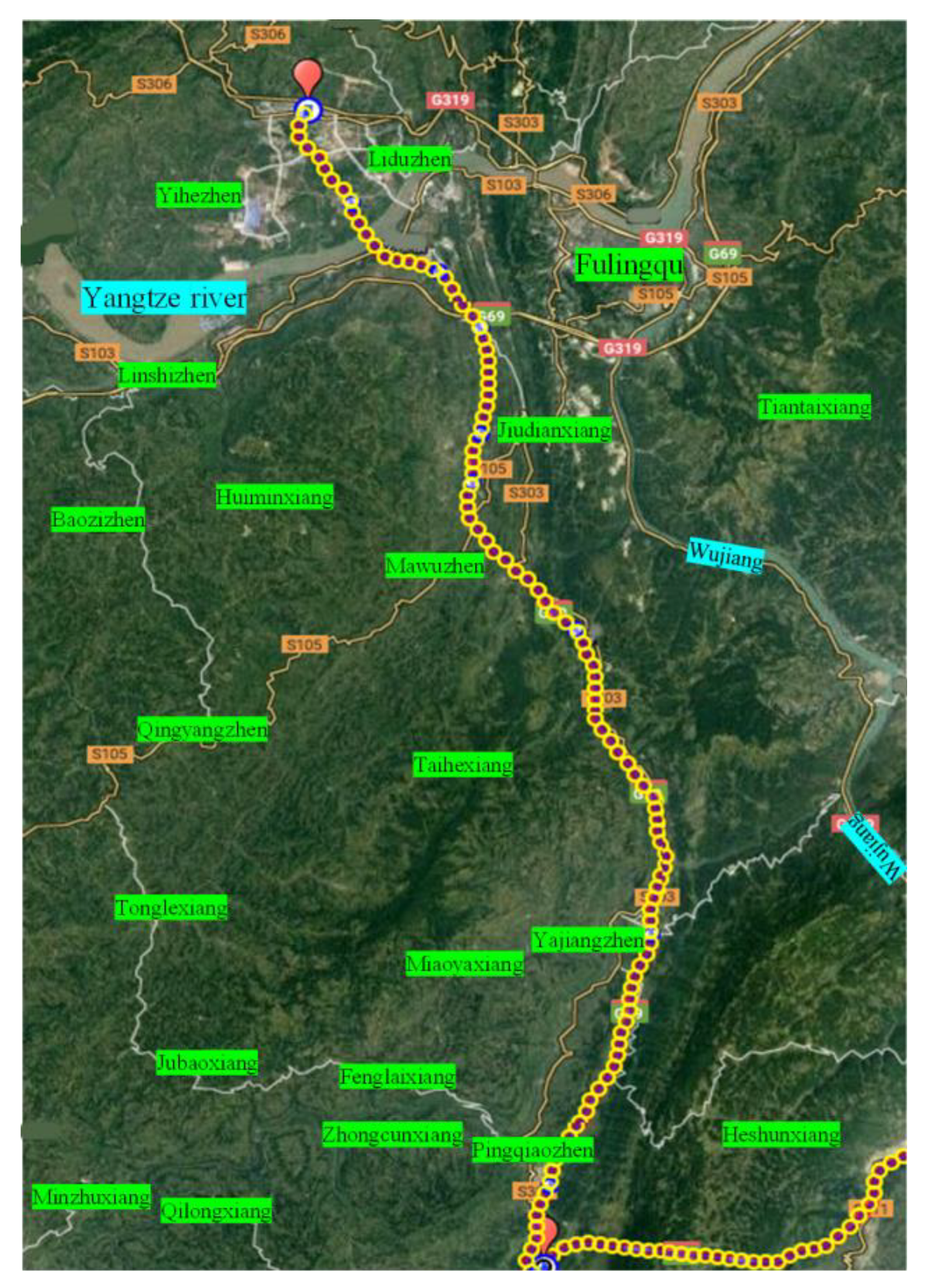
- A set of back-calculation methods based on a microelement method and cluster analysis of road geometric alignment was proposed in this study, and a 55 km highway was selected to verify the reliability of the method. The results showed that the back-calculated values of the flat curve length, flat curve deflection angle, longitudinal slope length, and longitudinal slope gradient were significantly correlated with the designed values. In addition, the correlation between the back-calculated values of the flat curve radius and the design value was improved significantly after stripping the outliers based on cluster analysis.
- (2)
- The section unit length, straight-line segment length, flat curve radius, flat curve deflection angle, longitudinal slope gradient, longitudinal slope length, and slope difference were selected as the input variables of the model, and the fitted prediction models were established by using the negative binomial regression and multilayer perceptron algorithm. Furthermore, the prediction accuracy of the model was evaluated by using the overall relative error, mean absolute deviation, cumulative residual, and correlation coefficient. The results showed that the prediction accuracy of the MLP model was better than that of the negative binomial model, and the evaluation indices were 3.2%, 0.371, 193.38, and 0.581, respectively.
- (3)
- SHAP theory was used to visualize the internal mechanism of action of the MLP model, and the results showed that only the road section unit length was monotonically and positively correlated with the accident frequency; the other characteristic variables exhibited complex nonlinear relationships with the accident frequency. Compared with the negative binomial model, the MLP model can estimate the complex nonlinear relationship between the independent and dependent variables more accurately and flexibly and can thus obtain a higher prediction accuracy.
- (4)
- In a future study, a comprehensive evaluation of road infrastructure accident risks will be conducted by introducing additional features, such as traffic flow and road cross-sections.
Author Contributions
Funding
Institutional Review Board Statement
Informed Consent Statement
Data Availability Statement
Conflicts of Interest
References
- Shah, S.A.R.; Ahmad, N.; Shen, Y.; Pirdavani, A.; Basheer, M.A.; Brijs, T. Road safety risk assessment: An analysis of transport policy and management for low-, middle-, and high-income Asian countries. Sustainability 2018, 10, 389. [Google Scholar] [CrossRef] [Green Version]
- World Health Organization. Global Status Report on Road Safety 2018: Summary; World Health Organization: Geneva, Switzerland, 2018. [Google Scholar]
- Fayard, G. Road injury prevention in China: Current state and future challenges. J. Public Health Policy 2019, 40, 292–307. [Google Scholar] [CrossRef]
- Wang, X.; Yu, H.; Nie, C.; Zhou, Y.; Wang, H.; Shi, X. Road traffic injuries in China from 2007 to 2016: The epidemiological characteristics, trends and influencing factors. PeerJ 2019, 7, e7423. [Google Scholar] [CrossRef] [Green Version]
- Wang, C.; Quddus, M.A.; Ison, S.G. The effect of traffic and road characteristics on road safety: A review and future research direction. Saf. Sci. 2013, 57, 264–275. [Google Scholar] [CrossRef]
- Lord, D.; Qin, X.; Geedipally, S. Highway Safety Analytics and Modeling; Elsevier: Amsterdam, The Netherlands, 2021. [Google Scholar]
- Horberry, T.; Anderson, J.; Regan, M.A.; Triggs, T.J.; Brown, J. Driver distraction: The effects of concurrent in-vehicle tasks, road environment complexity and age on driving performance. Accid. Anal. Prev. 2006, 38, 185–191. [Google Scholar] [CrossRef]
- Babkov, V.F. Road Conditions and Traffic Safety; National Academy of Sciences: Washington, DC, USA, 1975. [Google Scholar]
- Pei, Y.; Ma, J. Transport. Research on countermeasures for road condition causes of traffic accidents. China J. Highw. Transp. 2003, 16, 77–82. [Google Scholar]
- Ji, M.; Jiang, B.; Chen, S.; Li, H. Design and Research of Civil Engineering Courses under the Guidance of “The Belt and Road” Strategy Based on Craftsman Spirit. In Proceedings of the 2019 International Conference on Management, Education Technology and Economics (ICMETE 2019), Fuzhou, China, 25–26 May 2019; pp. 492–495. [Google Scholar]
- Zhao, L.; Liu, Z.; Mbachu, J. Highway alignment optimization: An integrated BIM and GIS approach. ISPRS Int. J. Geo-Inf. 2019, 8, 172. [Google Scholar] [CrossRef] [Green Version]
- Pei, Y.-L.; He, Y.-M.; Ran, B.; Kang, J.; Song, Y.-T. Horizontal Alignment Security Design Theory and Application of Superhighways. Sustainability 2020, 12, 2222. [Google Scholar] [CrossRef] [Green Version]
- Jovanis, P.P.; Chang, H.-L. Modeling the relationship of accidents to miles traveled. Transp. Res. Rec. 1986, 1068, 42–51. [Google Scholar]
- Joshua, S.C.; Garber, N.J. Estimating truck accident rate and involvements using linear and Poisson regression models. Transp. Plan. Technol. 1990, 15, 41–58. [Google Scholar] [CrossRef]
- Miaou, S.-P.; Hu, P.S.; Wright, T.; Rathi, A.K.; Davis, S.C. Relationship between truck accidents and highway geometric design: A Poisson regression approach. Transp. Res. Rec. 1992, 10–18. [Google Scholar]
- Miaou, S.-P. The relationship between truck accidents and geometric design of road sections: Poisson versus negative binomial regressions. Accid. Anal. Prev. 1994, 26, 471–482. [Google Scholar] [CrossRef] [PubMed] [Green Version]
- Milton, J.; Mannering, F. The relationship among highway geometrics, traffic-related elements and motor-vehicle accident frequencies. Transportation 1998, 25, 395–413. [Google Scholar] [CrossRef]
- Lord, D.; Mannering, F. The statistical analysis of crash-frequency data: A review and assessment of methodological alternatives. Transp. Res. Part A Policy Pract. 2010, 44, 291–305. [Google Scholar] [CrossRef] [Green Version]
- Wang, C.; Chen, F.; Cheng, J.; Bo, W.; Zhang, P.; Hou, M.; Xiao, F. Random-Parameter Multivariate Negative Binomial Regression for Modeling Impacts of Contributing Factors on the Crash Frequency by Crash Types. Discret. Dyn. Nat. Soc. 2020, 2020, 6621752. [Google Scholar] [CrossRef]
- Ferreira-Vanegas, C.M.; Vélez, J.I.; García-Llinás, G.A. Analytical methods and determinants of frequency and severity of road accidents: A 20-year systematic literature review. J. Adv. Transp. 2022, 2022, 7239464. [Google Scholar] [CrossRef]
- Islam, A.; Haque, B.; Hasan, J.; Amin, R. Frequency Modelling and Risk Evaluation of Road Crashes in Sylhet Region of Bangladesh. Int. J. Intell. Transp. Syst. Res. 2021, 20, 90–102. [Google Scholar] [CrossRef]
- Theofilatos, A. Utilizing Real-time Traffic and Weather Data to Explore Crash Frequency on Urban Motorways: A Cusp Catastrophe Approach. Transp. Res. Procedia 2019, 41, 471–479. [Google Scholar] [CrossRef]
- Wu, P.; Meng, X.; Song, L. A novel ensemble learning method for crash prediction using road geometric alignments and traffic data. J. Transp. Saf. Secur. 2019, 12, 1128–1146. [Google Scholar] [CrossRef]
- Thakali, L.; Fu, L.; Chen, T. Model-Based Versus Data-Driven Approach for Road Safety Analysis: Do More Data Help? Transp. Res. Rec. J. Transp. Res. Board 2016, 2601, 33–41. [Google Scholar] [CrossRef]
- Li, P.; Abdel-Aty, M.; Yuan, J. Real-time crash risk prediction on arterials based on LSTM-CNN. Accid. Anal. Prev. 2020, 135, 105371. [Google Scholar] [CrossRef]
- Lee, J.; Yoon, T.; Kwon, S.; Lee, J. Model Evaluation for Forecasting Traffic Accident Severity in Rainy Seasons Using Machine Learning Algorithms: Seoul City Study. Appl. Sci. 2019, 10, 129. [Google Scholar] [CrossRef] [Green Version]
- Wang, J.; Song, H.; Fu, T.; Behan, M.; Jie, L.; He, Y.; Shangguan, Q. Crash prediction for freeway work zones in real time: A comparison between Convolutional Neural Network and Binary Logistic Regression model. Int. J. Transp. Sci. Technol. 2022, 11, 484–495. [Google Scholar] [CrossRef]
- Lambert, D. Zero-inflated Poisson regression, with an application to defects in manufacturing. Technometrics 1992, 34, 1–14. [Google Scholar] [CrossRef]
- Winkelmann, R. Seemingly unrelated negative binomial regression. Oxf. Bull. Econ. Stat. 2000, 62, 553–560. [Google Scholar] [CrossRef]
- Hilbe, J. Negative Binomial Regression; Cambridge University Press: Cambridge, UK, 2011. [Google Scholar]
- Rosenblatt, F. The Perceptron, a Perceiving and Recognizing Automaton Project Para; Cornell Aeronautical Laboratory: Buffalo, NY, USA, 1957. [Google Scholar]
- Velo, R.; López, P.; Maseda, F. Wind speed estimation using multilayer perceptron. Energy Convers. Manag. 2014, 81, 1–9. [Google Scholar] [CrossRef]
- Lundberg, S.M.; Lee, S.-I. A unified approach to interpreting model predictions. In Proceedings of the 31st International Conference on Neural Information Processing Systems, Red Hook, NY, USA, 4–9 December 2017; p. 30. [Google Scholar]
- Yang, C.; Chen, M.; Yuan, Q. The application of XGBoost and SHAP to examining the factors in freight truck-related crashes: An exploratory analysis. Accid. Anal. Prev. 2021, 158, 106153. [Google Scholar] [CrossRef]
- Parsa, A.B.; Movahedi, A.; Taghipour, H.; Derrible, S.; Mohammadian, A.K. Toward safer highways, application of XGBoost and SHAP for real-time accident detection and feature analysis. Accid. Anal. Prev. 2020, 136, 105405. [Google Scholar] [CrossRef]
- Ribeiro, M.T.; Singh, S.; Guestrin, C. “Why should i trust you?” Explaining the predictions of any classifier. In Proceedings of the 22nd ACM SIGKDD International Conference on Knowledge Discovery and Data Mining, San Francisco, CA, USA, 13–17 August 2016; pp. 1135–1144. [Google Scholar]
- Štrumbelj, E.; Kononenko, I. Explaining prediction models and individual predictions with feature contributions. Knowl. Inf. Syst. 2014, 41, 647–665. [Google Scholar] [CrossRef]


| Road Section | Statistical Mileage/km | Number of Accidents | Number of Deaths | Number of Injured | Direct Property Damage/Million Yuan |
|---|---|---|---|---|---|
| Baomao highway | 501.1 | 7483 | 246 | 2405 | 13,248 |
| Hulong highway | 352.5 | 2455 | 94 | 803 | 2156 |
| Lanhai highway | 229 | 13,404 | 138 | 1988 | 17,196 |
| Yinkun highway | 112.2 | 13,097 | 85 | 1755 | 11,374 |
| Total | 1194.8 | 36,439 | 563 | 6951 | 43,974 |
| Calculated Values | Design Value | ||||
|---|---|---|---|---|---|
| Length of Flat Curve | Deflection Angle of Flat Curve | Radius of Flat Curve | Length of Longitudinal Slope | Slope of the Longitudinal Slope | |
| length of flat curve | 0.89 ** | −0.29 | 0.03 | — | — |
| deflection angle of flat curve | −0.14 | 0.96 ** | −0.52 ** | — | — |
| radius of flat curve | 0.06 | −0.33 * | 0.30 | — | — |
| length of longitudinal slope | — | — | — | 0.95 ** | 0.05 |
| slope of the longitudinal slope | — | — | — | 0.10 | 0.94 ** |
| Radius of Flat Curve | Maximum (/km) | Average Value (/km) | Minimum (/km) | Error (/%) |
|---|---|---|---|---|
| calculated values | 11.29 | 2.54 | 0.56 | 64.94 |
| design value | 3.60 | 1.54 | 0.79 |
| Independent Variable | Variable Symbols | Unit | Average Value | Standard Deviation | Minimum Value | Maximum Value |
|---|---|---|---|---|---|---|
| accident frequency | - | several cases per year | 0.48 | 0.52 | 0 | 2.57 |
| length of road section | L | km | 0.51 | 0.33 | 0.12 | 2.9 |
| length of straight section | Sl | km | 0.17 | 0.27 | 0 | 2.4 |
| flat curve radius | Hcr | 10 km | 3.52 | 4.65 | 0.0136 | 10 |
| deflection angle of flat curve | Hca | ° | 14.63 | 18.26 | 0 | 97.83 |
| longitudinal slope gradient | Vcg | % | 1.26 | 3.71 | −4.2 | 4. |
| longitudinal slope length | Vl | km | 1.22 | 0.92 | 0.15 | 4.6 |
| slope difference | Gd | % | 1.69 | 4.71 | 0 | 8.7 |
| Hyperparameter | Range | Value |
|---|---|---|
| Learning Rate | 0.00001, 0.0001, 0.001, 0.01, 0.1 | 0.001 |
| Batch Size | 16, 32, 64 | 32 |
| Optimization Function | SGD,Adam,RMSprop | Adam |
| Number of hidden layers | 2, 4, 6, 8 | 4 |
| Number of monolayer neurons | 40, 60, 80, 100, 120, 140 | 120 |
| Maximum number of iterations | 250, 300, 350, 400, 450, 500 | 450 |
| Negative Binomial Model | MLP | ||||
|---|---|---|---|---|---|
| Variables | Coefficient | Standard ErrOR | p Value | RI | Rank |
| L | 0.931 | 0.078 | 0.000 | 0.151 | 1 |
| Sl | 0.157 | 0.076 | 0.039 | 0.035 | 4 |
| Vcg | −0.113 | 0.751 | 0.880 | 0.022 | 6 |
| Hcr | −0.050 | 0.008 | 0.000 | 0.053 | 2 |
| Vl | 0.048 | 0.019 | 0.012 | 0.026 | 5 |
| Gd | 0.010 | 0.652 | 0.987 | 0.017 | 7 |
| Hca | −0.004 | 0.002 | 0.041 | 0.045 | 3 |
| _cons | −1.123 | 0.060 | 0.000 | —— | —— |
| α | 0.151 | 0.041 | —— | —— | —— |
| Evaluation metrics | |||||
| ORE | 3.5% | 3.2% | |||
| MAD | 0.441 | 0.371 | |||
| CSR | 216.609 | 193.380 | |||
| ρY,Y′ | 0.436 | 0.581 | |||
Disclaimer/Publisher’s Note: The statements, opinions and data contained in all publications are solely those of the individual author(s) and contributor(s) and not of MDPI and/or the editor(s). MDPI and/or the editor(s) disclaim responsibility for any injury to people or property resulting from any ideas, methods, instructions or products referred to in the content. |
© 2023 by the authors. Licensee MDPI, Basel, Switzerland. This article is an open access article distributed under the terms and conditions of the Creative Commons Attribution (CC BY) license (https://creativecommons.org/licenses/by/4.0/).
Share and Cite
Yan, J.; Zeng, S.; Tian, B.; Cao, Y.; Yang, W.; Zhu, F. Relationship between Highway Geometric Characteristics and Accident Risk: A Multilayer Perceptron Model (MLP) Approach. Sustainability 2023, 15, 1893. https://doi.org/10.3390/su15031893
Yan J, Zeng S, Tian B, Cao Y, Yang W, Zhu F. Relationship between Highway Geometric Characteristics and Accident Risk: A Multilayer Perceptron Model (MLP) Approach. Sustainability. 2023; 15(3):1893. https://doi.org/10.3390/su15031893
Chicago/Turabian StyleYan, Jie, Sheng Zeng, Bijiang Tian, Yuanwen Cao, Wenchen Yang, and Feng Zhu. 2023. "Relationship between Highway Geometric Characteristics and Accident Risk: A Multilayer Perceptron Model (MLP) Approach" Sustainability 15, no. 3: 1893. https://doi.org/10.3390/su15031893
APA StyleYan, J., Zeng, S., Tian, B., Cao, Y., Yang, W., & Zhu, F. (2023). Relationship between Highway Geometric Characteristics and Accident Risk: A Multilayer Perceptron Model (MLP) Approach. Sustainability, 15(3), 1893. https://doi.org/10.3390/su15031893