Noise Pollution Analysis Using Geographic Information System, Agglomerative Hierarchical Clustering and Principal Component Analysis in Urban Sustainability (Case Study: Tehran)

Abstract

In this study, a new approach has been used with SPSS and MATLAB analysis to study urban road traffic noise distribution mapping, to obtain the representative road traffic noise maps. The observation has been performed at a high traffic highway. The factors influencing noise level (traffic, road width, slope, and residential or administrative–commercial land) use were surveyed and recorded for each point and their local and time dependencies were computed. According to the analysis, the maximum value of goodness of fit index for the traffic and noise level relationship was 0.64, followed by 0.489 for the percentage of residential land use. The result of this study showed that the vehicle speed, width of the road, and the land use can affect different sound levels emitted by moving vehicles on road. The model predicts that by increasing one vehicle per hour, an increase in noise level by 0.002 dB will happen.

1. Introduction

Noise pollution has drawn attention to itself within the three recent decades, being a big problem in larger cities, and is seen as, collectively, being among the various environmental problems [1,2]. Studying this pollution and generating noise level maps for metropolises such as Tehran is of great importance. Subramani et al. analyzed pollution at different crossroads, generating a noise map via GIS [3].

A noise map in GIS is one of the best ways to recognize the sound of the environment. The study of noise maps is essential before presenting noise control policies, in order to investigate the distribution of existing noise levels and compare them with the standards of noise levels [4].

In other research in Iran, the urban noise survey revealed that, even in a medium size city such as Arak, environmental noise levels due to traffic are notably higher than the limits set by Iranian noise standards and policies to protect public health [5]. The time series has emerged as a response to the information evolution of chronological representation, where the information been made in time intervals [6]. Among the common clustering techniques is hierarchical clustering, which has been considered because it is the state of the art for various environmental and metrological data within the literature [7,8,9].

The study area consisted of a high traffic area of Hakim Highway. Noise measuring was supported with GIS software. It seems that the effect of traffic parameters and distance or proximity to residential areas on noise pollution is over other parameters, and is described in

Table 1. Research parameters for the study.

Research Question	Null Hypothesis
Is there a relationship between the speed of passing vehicles and the volume of traffic ?	Relation between speed and traffic volume is positive.
Is there a relationship between the use parameter of the buildings around the intersection and the volume parameter of passing vehicles?	Relation between the land use of buildings and the volume of the vehicles is positive.
Is there a relationship between the slope parameter and the noise?	Relation between the slope and the sound level is positive.
Is there a relationship between the road parameter and the noise?	Relation between the width of road and the sound level is positive.

. The use of statistical methods and spatial information systems bring us many benefits in pollution studies. At the end, the following questions about the research are responded to.

2. Research Methodology

Using noise measurement data, a sound pollution map of those points is ready, and within the next stage, using agglomerative hierarchical clustering (AHC) and principal component analysis (PCA), temporal and spatial analyses and effective components are performed. The results are summarized in the Figure 1.

Root Mean Square Error (RMSE) is the standard deviation of the residuals (prediction errors). Residuals are a measure of how far from the regression line data points are; RMSE is a measure of how spread out these residuals are.

First, various parameters involved in noise pollution were identified and their spatial data were generated as raster files to generate a pollution map. The parameters are the volume of vehicles, the slope of roads, urban land use, the width of road, and noise measurement data.

After collecting the data, they are analyzed in three sections, and spatial and temporal analyses are performed on them. Hakim Highway was selected based on its traffic and its urban importance. Measurements were performed during the evening time (1800–1900) for one week. In

Table 2. The summary of background research.

Author	Year	Country	Title
Bilaşco [10]	2017	Romania	GIS model for identifying urban areas vulnerable to noise pollution
Garg [11]	2017	India	Evaluation and analysis of environmental noise pollution in seven major cities of India
Gomez [12]	2016	Spain	Urban traffic noise and self reported health
Weber [13]	2014	Germany	Assessing modelled outdoor traffic-induced noise and air pollution around urban structures using the concept of landscape metrics
Abbaspour [14]	2015	Iran	Hierarchal assessment of noise pollution in urban areas
Khan, J. [15]	2018	Denmark	Assessment of exposure to air pollution and road traffic-review of tools and techniques
Monazzam Esmaeelpour [16]	2014	Iran	Designing a road traffic noise forecasting model for highways (Ahvaz City)

, the summary of the background research is described.

2.1. Influential Parameters in This Study

2.1.1. Slope

The mean slope of the study areas was 0–3%. To calculate the slope of the land, a scale of 1:2000 topographic map, prepared by the country’s surveying organization, was used. First, the points within the maps are entered into Civil3D 2014 Auto cad software, then a tier of the points is formed. A longitudinal profile is made ready on an element of the surface made by hand-recorded GPS (which is the same because of the noise level). The slope of the bottom is measured between noise measuring stations.

2.1.2. Land Use

For this purpose, first, the axis of the required route is determined and buildings at a distance of 100 m from either side of the axis of the route were examined. Figure 2 shows the sort of land use for Hakim Highway at a distance of 100 m from the highway axis.

For example, for use type information for the Hakim Highway area, see

Table 3. The amount of area and percentage of different uses in the area of Hakim Highway.

Total Area	Occupancy%	Area (Square Meters)	Occupation Level Title
	11	30,249.3	Residential
	32	91,457.9	Green Space
	9	25,140	Official
	48	140,045	Passages
	0	0	Commercial
286,892	100	286,892	Sum

.

2.1.3. Traffic

Traffic jams are not constant and change at different times. Therefore, measuring the volume of traffic at different time intervals is important. Changes in traffic volume at different times generally have a definite trend. Daily changes in traffic volume in all cities are generally similar to the following figure. As can be seen in the Figure 3, the daily traffic volume reaches its maximum in two times.

Morning peak hours: The hours during the morning when people usually attend work or when students attend educational centers. Rush hour, refers to the evening hours when people usually return home from work or from educational centers. The vehicle data were calculated using Equation (1) [18]:

$$V_a=V\times C_f$$

(1)

where V_a is traffic volume in a complete period (vehicle/h); V the calculated traffic during the measurement time in a period (vehicle/h); C_f the correction factor of the measurement (min/min). C_f is calculated via Equation (2):

$$C_f=\raisebox{1ex}{$T_c$}\!\left/ \!\raisebox{-1ex}{$T_c-T_s$}\right.$$

(2)

where $T_c$ is the complete measurement period (min); T_s the time for resting between measuring (min).

2.1.4. Road Width

Figure 4 shows two sections of the Hakim Highway, the widths of which are 18 m and 14.6 m.

2.1.5. Noise Modelling

The following assumptions were used in all calculations to provide both consistency and to conform to the limitations of 9613:

• A single point source and receiver were used for each calculation;
• The maximum horizontal source–receiver distance was 100 m;
• The ground was smooth and flat;
• There was no wind or atmospheric refraction (neutral atmosphere where rays of sound are straight);
• All calculations were performed as a function of frequency (1/3 octave bands) for 9613 and continuous for OTL Suite from 31.5 to 8000 Hz [19,20].

In connection with the characteristics of the sound source under evaluation, ISO 1996-2 establishes some aspects to be considered, but all of them concern the representativeness of the measure regarding the average conditions of the source in the environment and the variations in weather conditions. The possibility of an interaction between geometric and temporal aspects has not been raised [21].

3. Study Area

The Hakim Highway study area is located in District 2 of Tehran Municipality, which includes Hakim Highway with an east–west axis for harvesting operations. Hakim Highway, located in the center of Tehran, is one of the main thoroughfares of the capital and is located parallel to Shahid Hemmat Highway. This highway is approximately 9 km long and consists of 4 lanes or, in some routes, 3 lanes. Public places on the side of the highway are as follows:

Nezam Ganjavi Park, ASP Park, District 6 Municipality, Justice Complex, Seismological Center of Geophysical Institute, University of Tehran, Milad Hospital, Milad Tower, Milad Tower Pinball Center, road, Housing and Urban Development Research Center, Tehran Biodiversity Museum, Forest Park Pardisan, Aba Abdullah Mosque, Feyz Garden, Niloufar Park, Mulla Sadra Park, Milad Park, Olive Park, Noor Park, and Parvaz Park are some of the most important places located on the side of Hakim Highway.

In the figure below, this highway is distinguished from other roads by its blue color. Figure 5 shows the study area map of this area. Figure 6 shows the land use map of this area, which is distinguished by different colors.

The sound data were collected using the device TES Sound Level Meter 1353H (calibrated by a certified company). Measurements were performed at 15–20 m intervals. The longitudes and latitudes of every measurement point were recorded via a Garmin GPS device.

Raster polygon layers of noise measuring data for the studied area with ArcGIS 10.4.1 are presented in Figure 7. The details of the WGS (a standard used in cartography, geodesy, and satellite navigation including GPS) for the case study and the point are shown in Figure 5, Figure 6 and Figure 7.the minimum height is 1389 m and the maximum is 1410 m.

Regression Model

The study aimed to spot the correlation between noise and factors. Multivariate analysis may be a powerful method that permits one to look at the link between two or more variables of interest. Therefore, to know multivariate analysis fully, it is essential to grasp the subsequent terms [22].

In this research, noise level was a seamless variable and, because of the correlation of independent variables in the study, regression was used. The assumptions of regression toward the mean and linearity or nonlinearity of the link were tested. Values of the coefficient of correlation are always between −1 and +1. A correlation of +1 indicates that two variables are perfectly related in a positive linear sense; a correlation of -1 indicates that two variables are perfectly related during a negative linear sense, and a correlation of 0 indicates that there is no linear relationship between the variables [23]. It was critical to identify variable correlations in order to create the regression model, meaning the linear correlation of independent variables had to be less than 0.4 or 0.5, and correlations above 0.5 were either removed from the model or included with extra care and according to certain tests. Further, the constant variable and dependent variable had to have a high correlation. Therefore, as a descriptive variable for the dependent variable of noise level, the independent variable of traffic was a proper candidate for regression modeling. It was the same for road width variable; however, due to its high correlation (>0.8) with the traffic variable, it could not be used in the model. The slope variable also had a low correlation (~0.4) with the independent variable, and therefore was not suited for linear regression. From the land use variables, only the residential land use variable had a correlation of 0.64 with the noise level and was suited to modeling. However, residential land use variable also had a correlation above 0.5 with the traffic variable, which meant if both variables were modeled as independent variables, they had to undergo linear correlation analysis. Following these steps, the equation linearity analysis was performed to validate the model.

Significance of Estimated Parameters

Modeling was performed in SPSS25 using the linear regression via OLS (Ordinary Least Square) method. This section introduces the best two models and respective graphs and tests for confirming OLS assumptions. The tests were meant to verify the following:

• Verify goodness of fit;
• Parameter significance;
• No multi-collinearity;
• Normality of the residuals;
• Outlier data;
• Autocorrelation.

4. Results

Aim of this study is to determine the relationship between noise level using factors such as vehicle traffic, slope, width, and the percentage of residential, commercial, office, and natural land uses. For this purpose, the linear regression method was used. The correlation of the variables considered for the study is shown in the

Table 4. Correlation of the variables considered for the study.

	Morning Traffic	Morning Noise Level	Noon Traffic	Noon Noise Level	Evening Traffic	Evening Noise Level	Slope (%)	Residential Use(%)	Commercial Use (%)	Official Use (%)	Natural Use (%)	Width (m)
Morning traffic	1	0.6931	0.9998	0.5579	0.9960	0.5263	−0.5235	−0.6140	0.1575	−0.6536	0.5788	0.8285
Morning noise level			0.6911	0.9532	0.6975	0.9418	−0.4349	−0.6486	−0.1258	−0.3095	0.5876	0.6242
Noon traffic			1	0.5554	0.9950	0.5242	−0.5242	−0.6127	0.1607	−0.6537	0.5796	0.8352
Noon noise level				1	0.5590	0.9528	−0.3173	−0.4962	−0.3053	−0.3257	0.5626	0.5343
Evening traffic					1	0.5316	−0.5131	−0.6215	0.1609	−0.6490	0.5713	0.8164
Evening noise level						1	−0.3419	−0.4342	−0.0701	−0.2276	0.3559	0.4508
Slope(%)							1	0.4659	−0.1251	0.0749	−0.2807	−0.5469
Residential use(%)								1	0.7150	0.1750	−0.7782	−0.5731
Commercial use (%)									1	0.5570	−0.5012	−0.6800
Official use (%)										1	−0.3898	−0.6015
Natural use (%)											1	0.7075
Width (m)												1

.

4.1. Regression Models and Root Mean Square Error

Statistical analysis was performed to extract the linear equation between the parameters using the least common squares. The sound level parameter was evaluated as a dependent variable (L_eq) with other parameters for evening time:

• Seven parameters (traffic, slope, residential, commercial, office, green space and road width); The modeling result formula is shown below:
• Morning: $L_{eq}=0.002*Traffic+11.630*Slope-23.050*Residential-40.352*Commerical-7.456*Administrative-30.230*Natural Ground+0.0146*Road Width+78.592$; RMSE = 0.280;
• Noon: $L_{eq}=0.002*Traffic+10.263*Slope-15.606*Residential-47.440*Commerical-8.277*Administrative-23.843*Natural Ground+0.093*Road Width+79.189$; RMSE = 0.277;
• Evening: $L_{eq}=0.001*Traffic+10.857*Slope-20.319*Residential-38.093*Commerical-10.382*Administrative-36.552*Natural Ground+0.159*Road Width+81.007$; RMSE = 0.263.

From the information that uses for the parameters and noise map, three models have been calculated, and the noise level can be calculated in the morning, noon, and evening times. The stepwise models also allows for the use of all possible models.

For the obtained equations, the deviation from the mean squares (RMSE) of each equation was calculated, which is about 0.3.

After testing the regression model, the most effective model was selected using above formula, where L_eq is the background level (dB).

Fortunately, it seems that the t-test is applicable to a range of problems. Particularly, it is applicable to the matter of testing the statistical significance of a parametric statistic. The t-test shows the importance of a parametric statistic. In multivariate analysis, we are often fascinated by the easy question of whether or not there is a linear relationship between two variables within the population. Stated in statistical jargon, we wish to check the null hypothesis that the population parametric statistic for the regression of a variable on an experimental variable is capable zero [24]. The F-test (as the t-test) may also be used for tiny data sets, in contrast to the big sample chi-square tests (and large sample Z-tests), but require additional assumptions of normally distributed data (or error terms) [25].

In the F-test, the zero assumption means all parameters are zero at the same time. If rejected, it means all parameters do not simultaneously have zero values. The statistical values of the test are as follows:

$$F\left(test\right)=298.983$$

$$Prob>F=0.0000$$

Therefore, the zero assumption is rejected, indicating that at the significance level of 0.01, not all parameters are zero. The t-test was used to verify parameter significance, where the zero assumption indicates the tested parameter is insignificant at the respective level of significance.

The Cook’s distance was calculated for every observation in order to control outlier data. Data with Cook’s distances above 4/n were classified as outlier data. Due to the indicated measurement errors, the number of observations were reduced from 324 to 282.

Therefore, due to the fact that this issue is due to instrumental measurement error, it was retained in the observations. The t-test and F-test are computed for the parameters, and the example is as in

Table 5. Summary of model with t-test and F test.

Durbin-Watson Test	Statistics Summary					Standard Estimation Error	R2	R	Model
	F Meaning	Freedom Degree 2	Freedom Degree 1	F-Test	R2 Difference
1.811	0/000	280	1	497.107	0.640	2.8233	0.640	0.800	1
1.936	0/000	279	1	36.980	0.042	2.6577	0.682	0.826	2

and

Table 6. The F test and Analysis variance.

Model		Sum of Squares	Freedom Degree	F	Meaning
1	regression	3962.474	1	497.107	0.000
	residual	2231.897	280
	sum	6194.371	281
2	regression	4223.677	2	298.893	0.000
	residual	1970.694	279
	sum	6194.371	281

, below.

4.2. Principal Component Analysis

The first component, or PC1, has the highest specific value, indicating that this component is most affected by noise sources. Due to the fact that these components are located in busy urban areas, the classification of streets in this component is affected by these sources of pollution, which are located with the greatest difference in all streets. Based on this, we can introduce PC1 as a component of noise pollution. That is, any street with more PC1 pollution is mainly affected by traffic, slope, and the width of the street.

In the second component, residential areas with a high negative coefficient, and the parameter of office premises with a high positive coefficient, showed a different reaction to other parameters. In the third component, commercial premises indicate the greatest impact of this component on noise pollution sources. Based on this, it can be said that for any street with more PC3, their pollution is mainly affected by commercial places. The fourth component of natural land shows the most vulnerability to this component of noise pollution sources.

Table 7. Participation of special vectors in principal component analysis (PCA) and rotational matrix of factor analysis along with special and their explanation percentage.

Parameter	PC1	PC2	PC3	PC4
Traffic	0/440	0/119	0/225	0/198
Sound level	0/441	0/157	0/093	0/205
Slope	−0/365	−0/343	−0/219	−0/122
Residential	−0/321	−0/472	−0/075	−0/307
Commercial	0/054	0/178	0/740	0/167
Administrative	0/207	0/687	0/054	0/204
Natural ground	−0/372	−0/090	−0/342	−0/406
Road width	0/432	0/276	0/160	0/118
Variance percent	0/463	0/176	0/167	0/120
Variance sum	0/463	0/639	0/806	0/925

shows the values of PC1 to PC4 coefficients for noise pollution parameters.

Therefore, the models made in the linear regression section are justifiable and are shown according to Figure 8, Figure 9, Figure 10, Figure 11, Figure 12, Figure 13 and Figure 14.

According to Figure 9 the R² for slope and noise level was 0.251.

According to Figure 10 and Figure 11, the values of R² for the residential and commercial land use and the noise level were 0.489 and 7.823 × 10⁻⁴, respectively, and it is shown that the commercial land use is less important on noise level.

According to Figure 12, the R² for the administrative land use and sound level was 0.163.

According to Figure 13, the R² for the residential land use and sound level was 0.485, and it is shown that the width is important and has a direct effect on sound level.

According to Figure 14, the R² for the natural ground and sound level was 0.395, and it is shown that the slope of natural ground is important and has direct effect on sound level.

Figure 15 shows the modeled nonlinear relationship between residential land use and the sound level dependent variable.

Figure 16 shows the modeled nonlinear relationship between commercial land use and the sound level dependent variable.

Figure 17 shows the modeled nonlinear relationship between administrative land use administrative and the noise level dependent variable.

Figure 18 shows the modeled nonlinear relationship between natural ground and the sound level dependent variable.

Figure 19 shows the modeled nonlinear relationship between road width and the sound level dependent variable.

Figure 20 shows the modeled nonlinear relationship between slope and the sound level dependent variable.

The regression model is suggested in

Table 8. Model Summary and Parameter Estimation for Slope of Figure 9 and Figure 20.

Equation	Model Summary			Estimation of Parameters
	R2	F	Meaning	Constant	b1	b2	b3
Linear	0/172	58/110	0/000	73/943	−0/373
Curve grade two	0/176	29/598	0/000	74/042	−0/326	−0/008
Curve grade three	0/188	21/379	0/000	74/345	−0/362	−0/046	0/003
Compound	0/163	58/520	0/000	73/864	0/995
Logarithmic	0/13	58/520	0/000	4/302	−0/005
Ln	0/373	58/520	0/000	73/864	−0/005

.

The common results of all temporal analyses (cumulative hierarchical cluster analysis, principal component analysis, regression analysis, and, finally, using the artificial neural network method) were confirmed. The use of statistical methods and spatial information systems (GIS) bring us many benefits in noise pollution studies. In this study, based on statistical methods (AHC, PCA, and regression, as well as the use of an artificial neural network), temporal analysis and spatial analysis were performed using a spatial information system.

5. Discussion

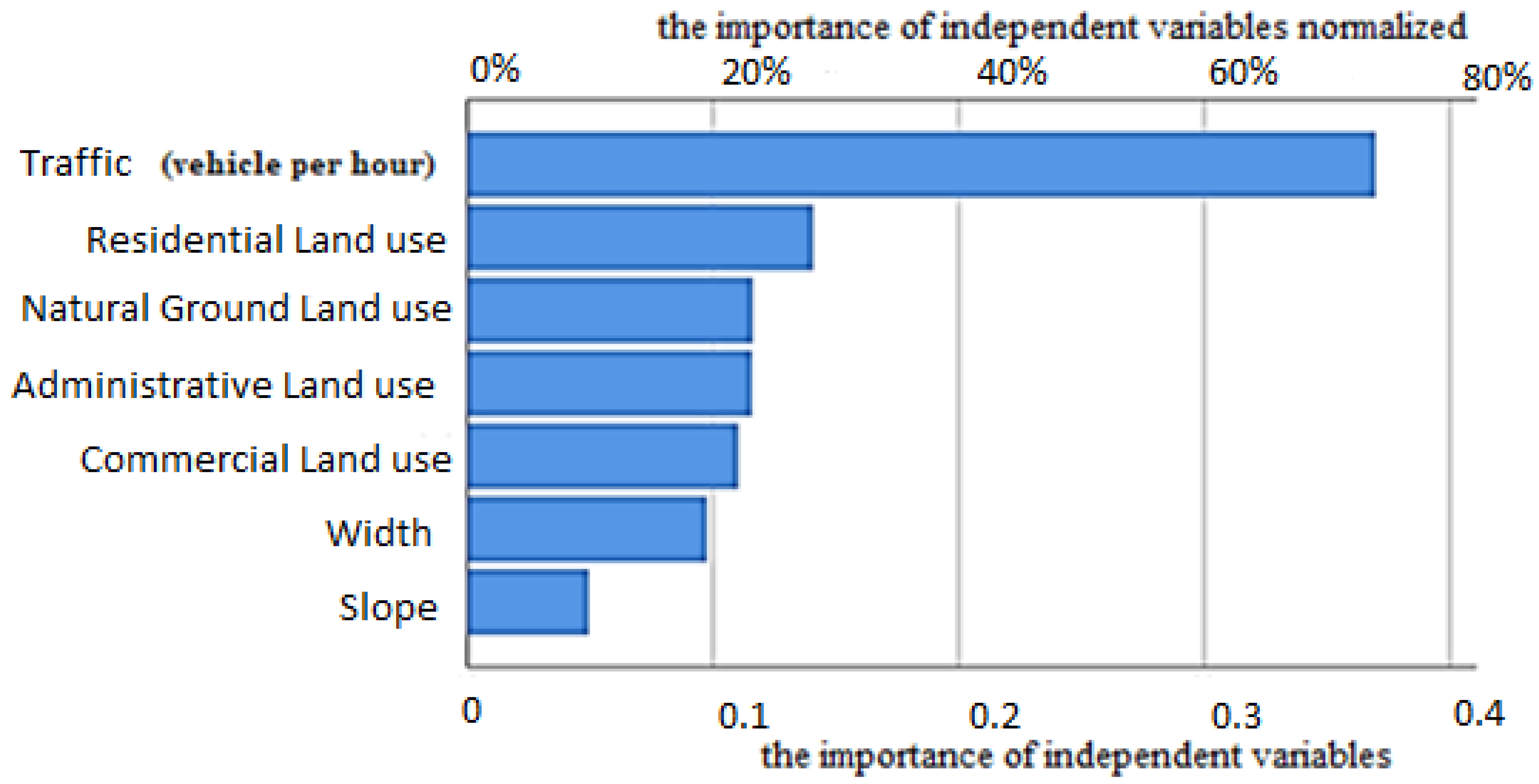
The role of traffic and residential use parameters in sound level were higher than other parameters. The following Figure 21 shows the importance of the independent variables in estimating the noise level dependent variable. As this figure shows, the volume of vehicle traffic is the most important, followed by the residential use variable. The linearity analysis was performed using a graph separating dependent and independent variables. The maximum value of goodness of fit index (R²) for the traffic and noise level relationship was 0.64, followed by 0.489 for the percentage of residential land use.

For comparing the results with the noise standard for different land uses,

Table 9. Outdoor permitted amount of noise in Iran [26].

Type of Area	Average Day Balance (7 am to 10 pm)	Average Night Balance (10 pm to 7 am)
Residential Area	55 dB	45 dB
Complex Area (Commercial–Residential)	60 dB	50 dB
Commercial–Administrative Area	65 dB	55 dB
Area of Activity (Residential–Industrial)	70 dB	60 dB
Industrial Zone	75 dB	65 dB

shows the environment standard of Iran, which is released by Department of Environment.

In the noise pollution map (Figure 6), the levels of sound pollution (red zones) belong to Hakim Highway. The findings suggest that the freeway function of Hakim areas and their relatively long distance from residential areas greatly influenced the resulting noise levels.

The results proved that noise maps would be effective instruments for understanding the distribution of the noise level in this study. Noise maps can be used to denote areas with high violation from standard. Cities such as Tehran, who are about to create a brand new sustainable urban lifestyle, have found that greenery could be a key element in addressing this pollution. Urban developers are currently attempting to find areas to plant vegetation. Hence, the greening of the façade of building walls, called vertical greenery systems (VGS), is gaining in popularity. The widespread use of vertical greenery systems on the many building walls in cities not only represents an excellent potential in reducing urban noises generated from traffic and machines, it is also a highly impactful way of mitigating the urban heat island effect and reworking the urban landscape.

6. Conclusions

The aim of this study was to investigate the effect of traffic parameters on the level of noise pollution near a highway in Tehran. There is a significant relationship in the modeling of Tehran due to the significance level of less than 0.05.

According to the common results of all time analyzes, which include “principal component analysis” and “regression analysis,” the noise level is more affected by the traffic volume and residential use parameters than other parameters. The relationship between sound level and traffic is direct, and with residential use it is inverse.

As can be seen in PC1 to PC4, the coefficients of the parameters of office and commercial premises are almost high (more than 0.6), which indicates that these two parameters are more effective in creating a difference between the streets than the other parameters. It should be noted that larger coefficients also include large negative coefficients. Therefore, for the streets that have a high value in terms of the first component, their noise pollution is affected by traffic, slope, and width of the street; in terms of the second component due to residential and office centers, in terms of the third component due to commercial places, and in terms of the fourth component, it is natural from the earth.

The results show that the land use is desensitized to traffic noise and fewer people perceive it as an annoyance in comparison of volume of traffic. The volume of vehicles are the significant factors for the propagation and increase in the traffic noise levels.

The issue of noise pollution in major cities of the world is considered as a pervasive issue, as it is one of the most important environmental problems today. In the last three decades it has received more attention in developed countries, but less in Iran when compared to other forms of environmental pollution. Some suggestions are given for reducing noise level in the urban areas, as below:

• In order to improve the quality of life of people in the residential land use in our study, noise pollution should be controlled.
• Use suitable sound walls in order to control noise pollution in the area.
• Increase the green space and parks around the study area to prevent the increase of noise pollution.
• Reduce traffic volume in the city by increasing traffic monitoring.
• Prevent the movement of vehicles, and use technical diagnosis for vehicles, that do not meet the required standards in order to reduce noise pollution.
• Increase the vegetation in the city to improve the environment.

The benefits of the calculation and evaluation of noise pollution distribution in the study area, especially in cities such as Tehran, are:

• Assigning of critical zones by reviewing noise maps.
• Evaluation of highway noise propagation into the adjacent districts, especially remedial, educational, research, and residential centers.
• Evaluation of the role of green belts and dense vegetation in the reduction of highway noise levels.
• Planning noise controls, such as noise barriers, in highways before and after construction, and evaluate the costs and the effects of noise control.