Abstract
In this paper, based on the traditional grey multivariate convolutional model, the concept of a buffer operator is introduced to construct a single-indicator buffered grey multivariate convolutional model applicable to air quality prediction research. The construction steps of the model are described in detail in this paper, and the stability of the model is analyzed based on perturbation theory. Furthermore, the model was applied to predict the air quality composite index of the “2 + 26” Chinese air pollution transmission corridor cities based on different socioeconomic development scenarios in a multidimensional manner. The results show that the single-indicator buffered grey multivariate convolutional model constructed in this paper has better stability in predicting with a small amount of sample data. From 2020 to 2025, the air quality of the target cities selected in this paper follows an improving trend. The population density, secondary industry, and urbanization will not have a significant negative impact on the improvement of air quality if they are kept stable. In the case of steady development of secondary industry, air quality maintained a stable improvement in 96.4% of the “2 + 26” cities. The growth rate of population density will have an inverted U-shaped relationship with the decline in the city air quality composite index. In addition, with the steady development of urbanization, air quality would keep improving steadily in 71.4% of the “2 + 26” cities.
1. Introduction
The overall air pollution situation in China has improved in recent years with the promulgation and implementation of environmental protection policies. However, serious air pollution still exists in many cities, such as the Beijing–Tianjin–Hebei (BTH) region and some of its surrounding cities. Air quality is always at a poor level because of industrial production and has an adverse effect on people’s quality of life. Some studies have shown that the loss of gross domestic product (GDP) from air pollution in various countries by 2060 will be particularly large in China [1]. Many scholars have devoted their research to prediction studies of air pollutant concentrations and other air-quality-related indicators. In addition, models that can yield higher accuracy prediction values are constantly being sought. Some of these studies are based on back propagation (BP) artificial neural network methods or their improvement for air quality prediction. Li (2014) proposed an air quality prediction method consisting of an iterative algorithm and a fuzzy BP neural network in order to improve the accuracy of air quality prediction, which effectively reduced the absolute value of the average prediction error [2]. Li et al. (2016) used an improved method based on wavelet analysis with a BP artificial neural network to predict the PM10 concentration of air pollutants and achieved better prediction results [3]. In addition, there are also swarm optimization algorithms [4], genetic algorithms [5,6], particle swarm optimization algorithms [7], and differential evolution algorithms [8], which are intelligent information-processing methods combined with BP artificial neural networks that can effectively improve model prediction precision and further contribute to air quality prediction research. There are also some studies that use traditional statistical models for air quality prediction, especially support vector machine-based air quality prediction. Li (2015) used wavelets to process the air quality index as well as air pollutants before using support vector machines for prediction analysis [9]. Both Li et al. (2018) and Chen and Li (2019) proposed a hybrid prediction model based on support vector regression. In order to reduce the non-smoothness of the series, the data of the system variable air pollutants were first processed. Different support vector machine models were built separately according to the different characteristics of the data, and the prediction results were obtained after the superposition operation. Thus, a better measurement effect was achieved [10,11]. In addition to support vector machines and their improved models, partial least squares regression, multiple linear regression, and integrated autoregressive moving average models have been used in air quality prediction studies [12,13,14].
The issue of air quality has attracted much attention and discussion in recent years. Initial research by scholars has revealed that some of the relevant data in this field have small sample sizes and missing records. In cases where statistical methods are used to predict the evolutionary trends of air quality, the problem of the inadequate characterization of regional influences on air quality often arises. In addition, traditional air quality statistical prediction methods have some inherent problems, such as neural networks requiring a vast amount of actual measurement data and being prone to overfitting. These problems can affect the quality of monitoring data analysis and the scientific accuracy and completeness of the prediction. The grey prediction model, as a model that can both consider the influence of relevant factors on the system changes and has characteristics applicable to the data, has also been widely used in air quality prediction studies with satisfactory results [15]. Xu et al. (2018) used a combination of a grey Markov model and a land use regression model to predict changes in PM10 concentrations [16]. Xiong et al. (2019) used an optimized grey extended prediction model to predict smog pollution in Shanghai and Beijing, China [17,18]. Shi and Wu (2021) introduced the Hausdorff derivative to the cumulative operator of the grey prediction model and the proposed new fractional-order grey prediction model was applied to predict the air quality indicators of cities [19]. The extensive use of grey prediction models in the field of air quality prediction not only provides further ideas for future research, but also establishes a solid theoretical foundation. The use of grey prediction models to analyze and predict air quality has become a hot research topic in this field. Since changes in air quality are a dynamic and natural evolution process, the prediction of air quality has a certain complexity.
For an accurate analysis of air quality development, not only breakthroughs in key technologies are needed, but also separate prediction models for different cities. In order to take into account the coordinated effects of social and economic systems in the prediction process, Professor Deng Julong proposed the GM(1,N) model for analyzing multivariate problems based on the traditional GM(1,1), in which the number of relevant factors is “N-1” [20]. Therefore, the research on multivariate grey models has been gradually developed. After a comparative analysis with previous models, it was found that the GM(1,N) model is similar to the GM(1,1) model in terms of characteristics. However, the prediction error of the GM(1,N) model is large and the modeling accuracy is still insufficient due to the fact that the grey differential equation has no exact solution in a practical sense. Additionally, problems such as imprecise time-response equations still exist [21]. In order to solve this problem, scholars have studied and improved multivariate grey prediction models from different perspectives and proposed the grey model GMC(1,N) with convolutional integration [22]. Its prediction results are more accurate than GM(1,N). However, the traditional grey prediction model suffers from data perturbation, and the prediction accuracy for fluctuating data is not high. Furthermore, there are problems such as the incomplete consideration of factors affecting air quality in the model prediction. All of these make the accuracy of traditional air quality prediction models limited. The widespread use of GMC(1,N) has exposed its drawbacks. The inconsistency in the discrete functions used for GMC(1,N) forecasting brings a large error to the model [23]. Therefore, to address the shortcomings in statistical prediction methods, this paper introduces the concept of a buffer operator based on the grey multivariate convolution model by considering the characteristics of factors influencing air quality from socioeconomic development and constructs a single-indicator buffered grey multivariate convolution model (SGMC(1,N)). It is built with a single-indicator buffered SGMC(1,N) after buffering the feature sequence with a weakened buffer operator. This paper also derives the perturbation bound of this model. The purpose of introducing the single indicator buffer is to seek the combination of quantitative prediction and qualitative analysis to mine the essential attributes of the data as well as to improve prediction accuracy. Thus, the practical value of the model is further improved, high-precision prediction analysis of urban air quality is achieved, and the air quality evolution law is revealed. The BTH region is the core region of China’s economic development. However, it is also the region with the most serious air pollution in China. Most previous studies have focused on the BTH region. Zhang et al. (2021) demonstrated that the combination of favorable meteorological conditions and anthropogenic emission reductions contributes to air quality improvement in the BTH region through the Community Multi-Scale Air Quality model [24]. Xu et al. (2022) predicted the air quality in the BTH region based on the coal conversion policy. The results showed that the concentrations of some air pollutants in the region will still be substandard by 2030 [25]. There are also seasonal predictions for air quality in the BTH region that explore the relationship between pollutant emissions and air quality changes [26]. However, the changes in air quality in this region are also affected by spillover effects from the surrounding areas. According to the 2017 Air Pollution Prevention and Control Work Plan for the BTH region and surrounding areas developed by the Chinese Ministry of Environmental Protection, “2 + 26” cities, including Beijing and Tianjin, as well as parts of Hebei Province and Henan Province, were identified as BTH-region air pollution transmission channel cities. There are relatively few studies on air quality in these “2 + 26” cities, and even fewer studies on air quality prediction based on the perspective of socioeconomic development in the region. In view of this, this study takes the Chinese air pollution transmission channel “2 + 26” cities as the research object.
In this paper, the air quality indexes of the “2 + 26” cities in the BTH region air pollution transmission corridor with different air quality conditions are predicted separately. Targeted suggestions are made to improve urban air quality. The study of the impact of socioeconomic development on air quality is beneficial to the green development of cities and has some reference significance for the formulation of environmental policies in China.
2. Grey Multivariable Convolution Model with a Single-Indicator Buffer
2.1. Modeling Process of SGMC(1,N)
The construction process of SGMC(1,N) is described as follows, and the main construction flow chart is shown in Figure 1.
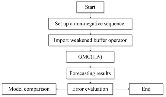
Figure 1.
The main construction process of SGMC(1,N).
The original non-negative sequence is obtained as the sequence under the action of the weakened buffer operator [27]. is generated by the first-order accumulation of the original sequence .
The matrix is calculated using the data generated by the first-order accumulation, and then the parameter is calculated according to the equation .
By substituting the parameters into the equation , the time-response equation of SGMC(1,N) is obtained (), in which the fitted and predicted values of the original series are calculated.
Mean absolute percent error (MAPE) is used as an error evaluation indicator. The calculation formula is shown below.
2.2. Stability Analysis of SGMC(1,N)
Based on the model perturbation theory, the stability of the model is discussed in terms of its perturbation bound. For SGMC(1,N), the perturbation bound is derived as follows.
Lemma 1.
[28] Assuming , the vector norm is compatible with the matrix norm . If there is for a matrix norm on , the solutions of the non-homogeneous linear equations and satisfy
Theorem 1.
Suppose that satisfies Lemma 1 and the unknown parameter of is x.
Proof.
If only perturbation occurs,
as well as
Therefore,
and,
Thus,
Therefore,
Because of
is obtained from Lemma 1. In other words,
If only perturbation occurs,
as well as
Thus,
By analogy, it can be obtained that
and
Therefore,
Because of
is obtained from Lemma 1. In other words,
Similarly, if only the perturbation occurs, the calculation procedure of the perturbation boundary is the same as above, and
can be obtained.
By the same token, if only occurs,
which means
It is observed that increases with the increment in the sample size m at a certain k. It implies that the perturbation bound of the solution enlarges when the sample size m grows. In other words, the sensitivity of to the solution will be positively correlated with the sample size . It shows that, when the sample size is relatively small, the perturbation bound of the solution is also smaller and the stability of the SGMC(1,N) model is better. Therefore, the SGMC(1,N) model is suitable for solving prediction problems with less data. □
3. AQCI Forecast for “2+26” Cities in China’s Air Pollution Transmission Corridor
The Chinese air pollution transmission channel “2 + 26” cities have a total area of about 27 × 104 km2, accounting for about 2.8% of the total area of the country, which is the core area of China’s economic development. The cities are densely populated and have a high urban traffic flow. In 2019, the resident population was about 189 million, accounting for roughly 13.6% of the country’s total population, and the total GDP was CNY 14.2 trillion, accounting for around 14.3% of the country. The region is dominated by heavy industrial development, with a high level of industrialization and high pollutant emissions, resulting in more serious pollution (the distribution of city locations is shown in Figure 2).
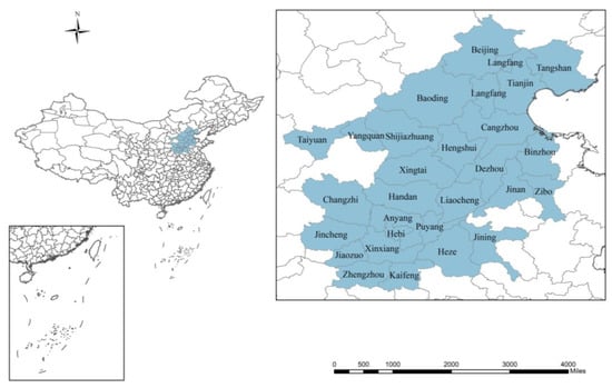
Figure 2.
Distribution of the city locations in the air pollution transmission corridor of the BTH region.
The AQCI, a national standard for evaluating air quality, provides a quantitative description of air quality. The index reflects the extent to which air is clean or polluted, and the resulting impact on human health. Based on the principles of scientificity, representativeness, operability, and timeliness, as well as combing and summarizing the relevant literature, in this paper, the following socioeconomic development factors that affect air quality were selected: industrial development [29], population pressure [30], and urbanization [31].
The value added by secondary industry is an indicator of industrial development. Secondary industry mainly includes industry and construction, and the economic growth of secondary industry may aggravate air pollution.
The population density of each city was used to respond to the impact of population pressure on air quality. Air quality is increasingly becoming a major inducer of population migration. Most of the areas with higher population densities have more employment opportunities and higher income levels, as well as relatively lower levels of air pollution. However, population growth also produces a number of problems such as increased energy consumption. Therefore, the impact of population density changes on air quality needs further investigation.
The urbanization ratio is an indicator that directly reflects the urbanization process. On the one hand, the development of urbanization is supported by a large amount of energy consumption, which is a major factor leading to the decrease in air quality. On the other hand, it also improves the level of environmental policy and raises public awareness of environmental protection. It can play a catalytic role in the improvement of air quality.
The indicators and units corresponding to each relevant factor are shown in Table 1. The data sources for the selected indicators in this paper were the Statistical Bulletin of National Economic and Social Development and the Statistical Yearbook of each city in the recent years.

Table 1.
Selection of socioeconomic development indicators.
Taking the prediction of the AQCI of Anyang, China, based on the secondary industry development scenario as an example, the specific model construction steps of SGMC(1,2) in practical application are as follows.
The sequence of systematic variables, is the AQCI of Anyang from 2013 to 2019, and the sequence is obtained under the action of the weakened buffer operator. The model calculations lead to
It can be derived by the least squares method that
The whitening equation of SGMC(1,2) is
and the time-response equation of SGMC(1,N) is obtained from the Gauss formula as
Thus, we can obtain the predicted AQCI of Anyang, China, with the added value of secondary industry as the relevant factor. The MAPE of SGMC(1,2) is 0.79%, which is lower than 10% (Table 2).
Table 2.
AQCI predictions for Anyang under the secondary industry development scenario.
This shows that the model is applicable to the calculation of AQCI in Anyang. In addition, the MAPE calculated using GMC(1,2) is 2.58%. It suggests that the accuracy of SGMC(1,2) is higher compared to that of GMC(1,2). The AQCI predictions for other cities were calculated using the same process as above. In the following, five cities were randomly selected from the “2 + 26” cities. Their AQCIs were fitted and calculated using different forecasting models (GM(1,N), GM(0,N), AGMC(1,N), and SGMC(1,N)). The fitting results and the MAPEs derived from each model are shown in Table 3. The results show that GM(1,N) has the lowest fitting accuracy, with three sets of data having MAPEs over 100%. GM(0,N) performs better than GM(1,N), but each set of data has MAPEs over 10%. Both AGMC(1,N) and SGMC(1,N) exhibited a relatively superior performance. SGMC(1,N) has the best performance, with the fitted MAPE value below 4% for each data set.
Table 3.
Fitting results and MAPEs of different models.
3.1. AQCI Prediction under the Secondary Industry Development Scenario
The AQCIs for the “2 + 26” cities under the secondary industry development scenario from 2020 to 2025 were obtained, and the results are shown in Table 4. The MAPEs obtained for all cities are lower than 10%, indicating that SGMC(1,2) is suitable for calculating this dataset.
Table 4.
AQCI predictions under the secondary industry development scenario.
The prediction results show that there is no significant negative impact on air quality improvement in most of the cities in the region selected in this paper when secondary industry maintains a stable development. The AQCIs of 19 cities will be reduced by more than 50% in 2025 compared to 2013 (Figure 3). However, there are still a few cities with an AQCI increasing annually or showing a rebound trend during the forecasting period. For example, the AQCI of Hebi shows a continuous increasing trend in the forecasting results. It increases to 8.34 by 2025, which is 27.55% higher than 2019. It shows that the negative impact of secondary industry development on air quality improvement is still present. The secondary sector includes industry and construction, where the burning of fossil fuels from industry and dust from construction are major contributors to air pollution. The rapid growth of the construction industry has promoted the development of industries, such as steel and cement, which not only directly affect urban air quality but also indirectly contribute to an increase in air pollution [32].
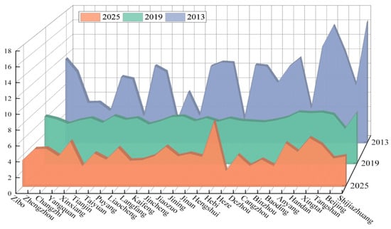
Figure 3.
AQCI comparison for the “2 + 26” cities (2013–2019–2025).
The severity of pollution levels in the cities of the region can be seen from the early raw data. Most cities with poor air quality in China are in a phase of rapid industrialization, with industrial energy consumption at a higher scale than other sectors. The rough industrialization pattern, especially the industrial structure dominated by heavy industry, has become a major obstacle to improving air quality. However, environmental regulation by the government and enterprises is constantly being urged; as the level of economic development of cities progresses, industry transforms and the level of technological innovation increases. All of these have contributed to the improvement of air quality.
3.2. AQCI Prediction under the Population Density Development Scenario
Since most of the “2 + 26” cities selected in this paper have small changes in population density, and the AQCI of each city shows an overall decreasing trend from 2013 to 2019, the AQCI of each city is predicted to maintain the trend of previous years according to the past development rate, and the AQCI of each city will decrease by 2025. In order to investigate the extent to which change in population density increase affects the AQCI, in this subsection, the change in the AQCI of each target city is calculated when the population density increase rate is 5% and 10%. The results show that an increase in population density can have a dramatic negative impact on urban air quality improvement. Taking the “2 + 26” cities Tianjin, Hengshui, Shijiazhuang, and Xingtai as examples, the AQCIs of these cities first show a decreasing trend when the population density increases at a 5% rate yearly, and then start to rebound in 2022 or 2023. When the population density growth rate is 10%, the AQCIs of the aforementioned four cities show a gradual increase over the forecasting years (Figure 4). In other words, the results of the AQCI prediction based on population density level show that an excessive increase in population density has a negative impact on the decrease in AQCI. The reason for this phenomenon is that an excessively rapid growth in the resident population leads to an increase in the demand for material goods. It implies an increase in the demand for resources and a significant increase in the demands on the environment. If the resident population becomes too large and demand exceeds the limits of environmental renewal, it can lead to ecological damage. This will inevitably affect air quality. The growth in population density will lead to an increase in waste emissions, both in domestic and production activities. Once the self-cleaning capacity of the atmosphere is exceeded, air pollution will be generated.
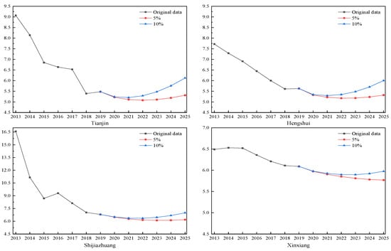
Figure 4.
AQCI prediction results for different population density growth rates.
3.3. AQCI Prediction under the Urbanization Development Scenario
The steady development of urbanization in most of the cities in the selected study area did not have a significant negative impact on air quality improvement. However, there are still cases in individual cities where air pollution is aggravated by the urbanization growth rate. For example, the AQCIs of Xingtai and Jining show a trend of decreasing and then increasing in the predicted years. The AQCI of Xingtai decreases to 6.45 in 2023 and then starts to rebound in 2024. Similarly, the AQCI of Jining also shows an increasing trend again in 2024. By contrast, the AQCIs of 26 cities, including Zibo, Zhengzhou, Shijiazhuang, Tianjin, and Taiyuan, decrease with urbanization and all manage to reduce to below 6 by 2025. This conclusion does not seem to be consistent with the current situation (Figure 5).
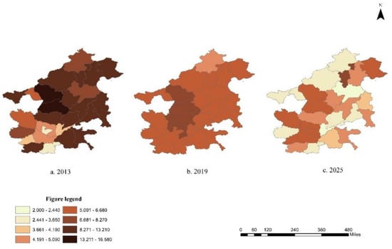
Figure 5.
Comparison of AQCIs (2013–2019–2025).
The AQCI in Shijiazhuang shows a non-linear change, increasing and then decreasing from 2013, but the urbanization rate is increasing year by year. This means that, at the current stage of development and with the increase in urbanization level, urban air pollution will potentially be aggravated. This view is also shared by some scholars. However, these scholars have not taken into account the following factors when analyzing air quality: First, air pollution levels are characterized by seasonal changes, and the decline in air quality generally accelerates during severe cold weather, especially in northern cities [33]. Winter heating in northern China requires the use of fossil fuels, and their emissions are the main cause of air pollution problems, such as haze. Second, urbanization has a strict demand for transportation and infrastructure construction, which will increase household energy consumption [34]. Increasing energy consumption will generate a vast amount of pollutants, which will eventually deteriorate the urban environment. Nevertheless, investments in environmental protection are currently increasing, especially in cities with high urbanization rates. The urbanization process will increase land use efficiency and energy consumption. Under government environmental regulation, residents will reduce the direct burning of fossil fuels, such as coal and oil [35,36], and increase the consumption of clean energy sources, such as electricity [37], which will eventually reduce pollutant emissions.
4. Conclusions
In order to extend the applicability of the GMC(1,N) model, this paper addressed multivariate grey forecasting theory and methods. Combined with the concept of a buffer operator, the single-indicator buffered SGMC(1,N) model was proposed. In addition, the problem of volatile data shocks perturbing system forecasting was solved. In the model construction section, the stability of the model was discussed by deriving the perturbation bound of SGMC(1,N). It is concluded that the model has a high stability in predicting with a small amount of sample data. In addition, four different computational methods, namely, GM(1,N), GM(0,N), AGMC(1,N), and SGMC(1,N), were used to fit the AQCI to randomly selected cities. It was demonstrated that SGMC(1,N) weakens the perturbation problem of unstable data shocks on the system prediction and possesses higher stability and prediction performance.
The practicality of the model constructed in this paper was demonstrated by an applied study conducted with the “2 + 26” cities of the Chinese air pollution transmission channel. This study demonstrated that population density, urbanization, and secondary industry development have important effects on the evolution of urban air quality.
There is no significant negative impact on air quality improvement when population density, secondary industry, and urbanization remain stable in most cities in the study area. Since the industrial structure has been adjusted in recent years, the level of government and enterprise coordination and environmental management performance has also gradually improved. Therefore, secondary industry maintaining a stable development is in line with the actual situation and development pattern of most of the “2 + 26” cities, which will not exhibit obvious negative air quality phenomena in 2020–2025. However, an excessive growth rate in population density will have a significant negative correlation with air quality in each city. The prediction results based on the perspective of urbanization development reveal that some cities will show a trend of AQCI first increasing and then decreasing during urbanization development. In other words, although urban air pollution may appear to increase with the increase in urbanization level, land use efficiency and energy consumption will be significantly improved with the further development of urbanization [38,39]. Furthermore, the urbanization process can promote economic development. With an increase in income level, people make higher demands on the environment, which can lead the government to strengthen urban greening and implement environmental policies. In addition, with the agglomeration of industries, cities can adopt more centralized treatment methods to deal with pollution emissions [40], which will effectively reduce air pollution. In these cities, developed economies and high income levels make environmental protection investments possible. Therefore, an increase in the urbanization rate and its association with low pollution is actually consistent with reality. Together with increased government regulations and the gradual improvement in environmental protection policies, it will effectively improve urban eco-efficiency and enable the further improvement of air quality [41]. This finding may be related to the time series in the study and the choice of regional differences.
Author Contributions
Conceptualization, K.S.; data curation, K.S. and Q.L.; formal analysis, K.S.; funding acquisition, H.L.; investigation, H.L. and L.Z.; methodology, K.S. and Q.L.; resources, K.S. and L.Z.; validation, K.S. and H.L.; visualization, L.Z.; writing—original draft, K.S. and Q.L.; writing—review and editing, K.S.; revision, K.S., L.Z. and Q.L. All authors have read and agreed to the published version of the manuscript.
Funding
This research was funded by the Tianjin Smart Manufacturing Special Funds Project, grant number 20201195.
Institutional Review Board Statement
Not applicable.
Informed Consent Statement
Not applicable.
Data Availability Statement
The data presented in this study are available on request from the corresponding author. The data are not publicly available due to the fact that one part is not publicly available at this stage.
Conflicts of Interest
The authors declare no conflict of interest. The funders had no role in the design of the study; in the collection, analyses, or interpretation of data; in the writing of the manuscript, or in the decision to publish the results.
References
- Lanzi, E.; Dellink, R.; Chateau, J. The sectoral and regional economic consequences of outdoor air pollution to 2060. Energy Econ. 2018, 71, 89–113. [Google Scholar] [CrossRef]
- Li, X. Air quality forecasting based on GAB and fuzzy BP neural network. J. Huazhong Univ. Sci. Technol. (Nat. Sci. Ed.) 2013, 41 (Suppl. S1), 63–65+69. [Google Scholar]
- Hu, J.; Yang, H.J.; Cheng, C. PM2.5 concentration prediction model based on BP neural network of improved artificial bee colony. J. Shandong Jiaotong Univ. 2020, 4, 15–22. [Google Scholar]
- Gan, L.Q.; Liu, Y.H. Air Quality Index Prediction Based on Outlier Detection and Error Correction. Comput. Syst. Appl. 2021, 3, 250–255. [Google Scholar]
- Gong, P.B.; Guo, H.P.; Duan, Z.S. Improved BP Neural Network Method for Predicting Environmental Radon Concentration. Nucl. Electron. Detect. Technol. 2019, 3, 279–284. [Google Scholar]
- Liang, Z.; Wang, Y.Y.; Yue, Y.W. A coupling model of genetic algorithm and RBF neural network for the prediction of PM2.5 concentration. China Environ. Sci. 2020, 40, 523–529. [Google Scholar]
- Zhao, G.Y.; Ma, F. Prediction of Dust Concentration Based on Particle Swarm Optimization BP Neural Network. Meas. Control Technol. 2018, 37, 20–23. [Google Scholar]
- Luo, S.Q.; Liu, H.T. Prediction of atmospheric pollution based on BP neural network optimized by hybrid algorithms. J. Nat. Sci. Heilongjiang Univ. 2020, 37, 389–394. [Google Scholar]
- Zhang, C.; Tang, W.; Xiao, J.; Tao, T.; Yuan, W.H.; Du, J.J.; Shu, y. Development and Application of Artificial Intelligence-Based System for Air Quality Prediction. Environ. Sci. Technol. 2020, 43 (Suppl. S2), 188–193. [Google Scholar]
- Li, J.G.; Luo, A.R.; Li, X.L. Prediction of PM2.5 Mass Concentration Based on Complementary Ensemble Empirical Mode Decomposition and Support Vector Regression. J. Beijing Univ. Technol. 2018, 44, 1494–1502. [Google Scholar]
- Chen, J.F.; Li, Y. Forecasting of PM2.5 concentration based on multimodal support vector regression. Environ. Eng. 2019, 37, 122–126+34. [Google Scholar]
- Sun, W.; Sun, J.Y. Daily PM2.5 concentration prediction based on principal component analysis and LSSVM optimized by cuckoo search algorithm. Environ. Manag. 2017, 188, 144–152. [Google Scholar]
- Shams, S.R.; Jahani, A.; Kalantary, S.; Moeinaddini, M.; Khorasani, N. The evaluation on artificial neural networks (ANN) and multiple linear regressions (MLR) models for predicting SO2 concentration. Urban Clim. 2021, 37, 100837. [Google Scholar] [CrossRef]
- Maciag, P.S.; Kasabov, N.; Kryszkiewicz, M.; Bembenik, R. Air pollution prediction with clustering-based ensemble of evolving spiking neural networks and a case study for London area. Environ. Model. Softw. 2019, 118, 262–280. [Google Scholar] [CrossRef]
- Tu, L.P.; Chen, Y. An unequal adjacent grey forecasting air pollution urban model. Appl. Math. Model. 2021, 99, 260–275. [Google Scholar] [CrossRef]
- Xu, S.; Zou, B.; Shafi, S.; Sternberg, T. A hybrid Grey-Markov/LUR model for PM10 concent ration prediction under future urban scenarios. Atmos. Environ. 2018, 187, 401–409. [Google Scholar] [CrossRef]
- Xiong, P.P.; Yan, W.J.; Wang, G.Z.; Pei, L.-L. Grey extended prediction model based on IRLS and its application on smog pollution. Appl. Soft Comput. 2019, 80, 797–809. [Google Scholar] [CrossRef]
- Xiong, P.P.; Shi, J.; Pei, L.L.; Ding, S. A novel linear time-varying GM(1,N) model for forecasting haze: A case study of Beijing, China. Sustainability 2019, 11, 3832. [Google Scholar] [CrossRef]
- Shi, K.H.; Wu, L.F. Modelling the relationship between population density and air quality using fractional Hausdorff grey multivariate model. Kybernetes 2021, 50, 3129–3150. [Google Scholar] [CrossRef]
- Ofosu-Adarkwa, J.; Xie, N.M.; Javed, S.A. Forecasting CO2 emissions of China’s cement industry using a hybrid Verhulst-GM(1,N) model and emissions’ technical conversion. Renew. Sustain. Energy Rev. 2020, 130, 109945. [Google Scholar] [CrossRef]
- Chen, H.; Xiao, X.P.; Wen, J.H. Novel multivariate compositional data’s model for structurally analyzing sub-industrial energy consumption with economic data. Neural Comput. Appl. 2020, 6, 3713–3735. [Google Scholar] [CrossRef]
- Zhang, Z.Y.; Wu, L.F.; Chen, Y. Forecasting PM2.5 and PM10 concentrations using GMCN(1,N) model with the similar meteorological condition: Case of Shijiazhuang in China. Ecol. Indic. 2020, 119, 106871. [Google Scholar] [CrossRef]
- Ma, X.; Liu, Z.B. The GMC(1,N) model with optimized parameters and its application. J. Grey Syst. 2017, 29, 122–138. [Google Scholar]
- Zhang, Y.B.; Chen, X.; Yu, S.C.; Wang, L.; Li, Z.; Li, M.; Liu, W.; Li, P.; Rosenfeld, D.; Seinfeld, J.H. City-level air quality improvement in the Beijing-Tianjin-Hebei region from 2016/17 to 2017/18 heating seasons: Attributions and process analysis. Environ. Pollut. 2021, 271, 116523. [Google Scholar] [CrossRef]
- Xu, M.; Zhang, S.H.; Xie, Y. Impacts of the clean residential combustion policies on environment and health in the Beijing–Tianjin–Hebei area. J. Clean. Prod. 2023, 384, 135560. [Google Scholar] [CrossRef]
- Zhang, Z.Y.; Zhao, X.J.; Mao, R.; Xu, J.; Kim, S.-J. Predictability of the winter haze pollution in Beijing–Tianjin–Hebei region in the context of stringent emission control. Atmos. Pollut. Res. 2022, 13, 101392. [Google Scholar] [CrossRef]
- Zhou, W.J.; Zhang, H.R.; Dang, Y.G.; Wang, Z.X. New information priority accumulated grey discrete model and its application. Chin. J. Manag. Sci. 2017, 25, 140–148. [Google Scholar]
- Dai, H. Matrix Theory; Science Press: Beijing, China, 2001. [Google Scholar]
- Shi, K.H.; Wu, L.F. Forecasting air quality considering the socio-economic development in Xingtai. Sustain. Cities Soc. 2020, 61, 102337. [Google Scholar] [CrossRef]
- Borck, R.; Schrauth, P. Population density and urban air quality. Reg. Sci. Urban Econ. 2021, 86, 103596. [Google Scholar] [CrossRef]
- Khan, I.; Hou, F.J.; Le, H.P.; Ali, S.A. Do natural resources, urbanization, and value-adding manufacturing affect environmental quality? Evidence from the top ten manufacturing countries. Resour. Policy 2021, 72, 102109. [Google Scholar] [CrossRef]
- Meda, U.S.; Vora, K.; Athreya, Y.; Mandi, U.A. Titanium dioxide based heterogeneous and heterojunction photocatalysts for pollution control applications in the construction industry. Process Saf. Environ. Prot. 2022, 161, 771–787. [Google Scholar] [CrossRef]
- Zhao, H.; Chen, K.Y.; Liu, Z.; Zhang, Y.; Shao, T.; Zhang, H. Coordinated control of PM2.5 and O3 is urgently needed in China after implementation of the “Air pollution prevention and control action plan”. Chemosphere 2021, 270, 129441. [Google Scholar] [CrossRef] [PubMed]
- Leveque, B.; Burnet, J.-B.; Dorner, S.; Bichai, F. Impact of climate change on the vulnerability of drinking water intakes in a northern region. Sustain. Cities Soc. 2021, 66, 102656. [Google Scholar] [CrossRef]
- Wright, C.; Nyberg, D.; Bowden, V. Beyond the discourse of denial: The reproduction of fossil fuel hegemony in Australia. Energy Res. Soc. Sci. 2021, 77, 102094. [Google Scholar] [CrossRef]
- Gyamfi, B.A.; Adedoyin, F.F.; Bein, M.A.; Bekun, F.V.; Agozie, D.Q. The anthropogenic consequences of energy consumption in E7 economies: Juxtaposing roles of renewable, coal, nuclear, oil and gas energy: Evidence from panel quantile method. J. Clean. Prod. 2021, 295, 126373. [Google Scholar] [CrossRef]
- Ahmed, Z.; Asghar, M.M.; Malik, M.N.; Nawaz, K. Moving towards a sustainable environment: The dynamic linkage between natural resources, human capital, urbanization, economic growth, and ecological footprint in China. Resour. Policy 2020, 67, 101677. [Google Scholar] [CrossRef]
- Cheng, Z.H.; Wang, L. Can new urbanization improve urban total-factor energy efficiency in China? Energy 2023, 266, 126494. [Google Scholar] [CrossRef]
- Su, M.; Wang, Q.; Li, R.R.; Wang, L. Per capita renewable energy consumption in 116 countries: The effects of urbanization, industrialization, GDP, aging, and trade openness. Energy 2022, 254, 124289. [Google Scholar] [CrossRef]
- Liang, L.W.; Wang, Z.B.; Li, J.X. The effect of urbanization on environmental pollution in rapidly developing urban agglomerations. J. Clean. Prod. 2019, 237, 117649. [Google Scholar] [CrossRef]
- Wang, Z.H.; Liu, B.; Wang, L.S.; Shao, Q. Measurement and temporal & spatial variation of urban eco-efficiency in the Yellow River Basin. Phys. Chem. Earth 2021, 122, 102981. [Google Scholar]


Disclaimer/Publisher’s Note: The statements, opinions and data contained in all publications are solely those of the individual author(s) and contributor(s) and not of MDPI and/or the editor(s). MDPI and/or the editor(s) disclaim responsibility for any injury to people or property resulting from any ideas, methods, instructions or products referred to in the content. |
© 2023 by the authors. Licensee MDPI, Basel, Switzerland. This article is an open access article distributed under the terms and conditions of the Creative Commons Attribution (CC BY) license (https://creativecommons.org/licenses/by/4.0/).