Spatial Vitality Evaluation and Coupling Regulation Mechanism of a Complex Ecosystem in Lixiahe Plain Based on Multi-Source Data

Abstract

[Purpose] With the acceleration of China’s urbanization process and the construction of the metropolitan area, the polarization phenomenon (Matthew effect) between cities and cities, cities and villages, and villages and villages has become increasingly prominent, and the relationship between urban and rural construction elements such as economy, society, nature, and population has become increasingly complex. However, due to the huge differences between cities and villages, it is difficult to use a unified “measuring ruler” to compare them horizontally and vertically in the space–time dimension. Therefore, it is necessary to evaluate and measure the spatial vitality of each administrative unit in the region from the perspective of urban development, that is, the sustainable development capacity of space. [Method] Taking Lixiahe Plain as the research object, based on the multi-source data such as POI, night-time light, and land use/cover, on the one hand, the spatial vitality evaluation system of the complex ecosystem is constructed, and the vitality levels and types of different township units are divided. On the other hand, the coupling degree model, coupling degree coordination degree model, spatial correlation analysis, and exploratory space–time data analysis are used to analyze the complex relationship and dynamic evolution characteristics of interaction stress among the spatial vitality of township units. [Conclusion] (1) The spatial vitality status is generally good, but there are great differences among regions, and the trend of fluctuant declines from west to east, and the spatial vitality type is a mainly vigorous type and development type. (2) There is a strong spatial dependence among the subsystems of the township units in the region. The spatial structure of the township units in the central area is more dynamic, while the spatial structure of the surrounding towns is more stable. (3) The 136 township units are divided into 4 different types of villages and towns, namely, coordinated evolution type, maladjustment evolution type, overall invariant type, and stable invariant type, which is conducive to putting forward their own development strategies.

1. Introduction

As a long-term basic national policy, the core of sustainable development is development, which requires economic development and social progress under the premise of strictly controlling the population, improving the population quality, protecting the environment, and the sustainable utilization of resources, etc. [1,2]. At present, China’s ecological environment protection and governance have achieved remarkable results. However, as the urbanization process entered the middle and late stages, this not only intensified the migration and mobility of the population but also caused the unbalanced development of education, medical care, employment, and other resources, making the regional differences between large, medium, and small cities and the urban–rural differences between cities and villages increasingly large [3,4,5]. For this reason, underdeveloped regions, small and medium-sized cities in the metropolitan area, and rural hinterland are all facing the dilemma of declining sustainable development capacity and development momentum. For example, unreasonable industrial structure and layout, uneven distribution of public service facilities, imperfect infrastructure construction, broken ecosystem balance, disordered urban function zoning planning, blind investment in rural land resources, and other issues are the main factors that cause the unsustainable economy, society, nature, and population [6,7,8].

The above factors together determine that the evaluation of the health and sustainable development of complex ecosystems have become a research hotspot in recent years, including the environmental carrying capacity, coordinated development degree, symbiosis degree and disaster resilience, and other research contents [9,10,11]. Emergy analysis, statistical analysis, the DEMATEL method, Morlet wavelet transform, data envelopment analysis, natural breakpoint classification, and other methods are used to select and measure indices [12,13]. In terms of research content, early studies focused on the sustainable development of human beings and their living ecological environment. There are few studies on the decline in the sustainable development ability of the economy, society, nature, and population caused by population, industry, location, and transportation in urban and rural areas. Among them, the research on the vitality of cities, streets, public spaces, and other spaces cannot be separated from the development of spatial structure theory, such as the exploration of urban form, function, context, environmental protection, and other issues [14,15,16,17]. In terms of research methods, early studies often used field surveys, questionnaire interviews, statistical yearbooks, and other traditional data types, which are highly subjective [18,19,20,21]. Others combined data with electronic maps, street view images, video surveillance, bus swipe cards, and other single temporal and spatial data to enhance the timeliness of data acquisition and analysis to a certain extent [22,23,24,25], but this is still not enough to support the systematic comparative analysis and research of numerous county units and township units in a large-scale space [26].

With the rapid progress of 3S technology and the popularization and development of the Internet, the Internet of Things, and other technologies, spatial vitality research has gradually evolved from a kind of data to the integration of multi-source, spatio-temporal big data, such as basic spatial data, dynamic monitoring data, positioning communication data, network media data, social network data, and credit card consumption data [27,28]. All kinds of spatio-temporal big data are increasingly becoming a new technical means for urban and rural planning, construction, and management research. The research content can be divided into three levels. The first level is to mine and analyze the spatio-temporal differentiation characteristics of urban and rural spatial vitality factors using multi-source spatio-temporal big data [29,30]. The second level is to discover the evolution rules and measure the gradient characteristics of urban and rural spatial vitality based on the spatio-temporal differentiation characteristics [31]. The third level is to explore the internal mechanism of coupling and coordination evolution based on the distribution and evolution characteristics of urban and rural spatial vitality [32,33]. This paper attempts to combine multi-temporal remote sensing images, land use/cover, POI, field research, and statistical yearbook data; to use RS, GIS, web crawler technology, and software platforms such as ENVI, ArcGIS, SPSS, and python to analyze the evolution and spatial pattern characteristics of the urban–rural complex ecosystem in the Lixihe Plain; to build an evaluation framework and evaluation model for the spatial vitality of the urban and rural composite ecosystem; and reveal the coupling mechanism of spatial vitality on an urban and rural complex ecosystem [34,35,36,37,38,39,40,41].

2. Materials and Methods

2.1. Study Area

Lixiahe Plain (118°28′48′′E–120°21′36′′E, 32°13′12′′N–34°7′12′′N) is located in the middle north region of Jiangsu Province, the most economically developed Province in China. It is north of the Yangtze River, south of the Huai River, and the Beijing-Hangzhou Grand Canal runs through it. The lake area in Lixiahe Plain accounts for about 43% of the total lake area in the Province. It is the concentrated distribution area of important freshwater marsh wetlands in China, the starting point of the eastern line of the South-to-North Water Diversion Project, and an important commodity grain base in Jiangsu Province. In a narrow sense, Lixiahe Plain is bounded by water, starting from Tongyu River in the east, reaching Li River in the west, old Tongyang Canal in the south, and ending at the Main Irrigation Channel of North Jiangsu in the north. It is an important component of the coastal plain and lake depression plain in North Jiangsu. According to the landform and water system, the area to the west of the Beijing-Hangzhou Grand Canal can be called the Western Lake Area; the area to the east of the Beijing Hangzhou Grand Canal and the area to the west of the Chuanchang River can be called the Central Lacustrine Area; and the area to the east of Chuanchang River can be called the coastal river network area. In a broad sense, Lixiahe Plain is bounded by administrative divisions, including 20 county units and 359 township units under the jurisdiction of 5 Municipalities divided into Districts, Nantong, Taizhou, Yangzhou, Yancheng and Huai’an. The Lixiahe Plain described in this paper combines the natural regional characteristics and the status quo of administrative division (Figure 1). As of December 2020, Lixiahe Plain covers an area of 27,341.08 km². It had a population of approximately 14.7660 million, a gross domestic product of approximately CNY 1427.728 billion, and a permanent resident population density of approximately 540 people/km². However, in recent years, the population loss in the study area is serious, and both the quantity and quality of the population are lower than the average value of various indicators in Jiangsu Province, which has become a “depression” for the development of Jiangsu Province.

2.2. Acquisition and Processing Method of Multi-Source Data

2.2.1. POI Data

Crawler technology can effectively solve the problems of low efficiency and timeliness, huge collection workload, and high cost of processing geographic information data collected in the traditional urban planning industry [42,43,44,45]. Among them, Point of Interest (POI) data contains a lot of geospatial information needed for research. Amap with a higher download efficiency is selected as the POI data source of this paper, and the classification code and the city code as defined by Amap are adopted. At present, there are 23 major categories, 267 medium categories, and 869 minor categories of POI classification codes. This research refers to the urban and rural spatial vitality indices obtained by domestic and foreign scholars and selects the spatial vitality elements of economic and social subsystems from the POI data.

2.2.2. Land Use/Cover Data

Land use/land cover data is an important basis for effectively monitoring the development and utilization of land resources and analyzing the changes in specific land types within the same spatial scope and long-term land series in specific areas [46,47]. In this paper, the land use/cover data are all from TM and ETM+sensors carried by Landsat 5 and Landsat 7, and the land resource classification standard led by the Institute of Geography, Chinese Academy of Sciences, is used as the natural vitality elements. Landsat data were downloaded from the United States Geological Survey, using the path number and row number of the Worldwide Reference System 2.

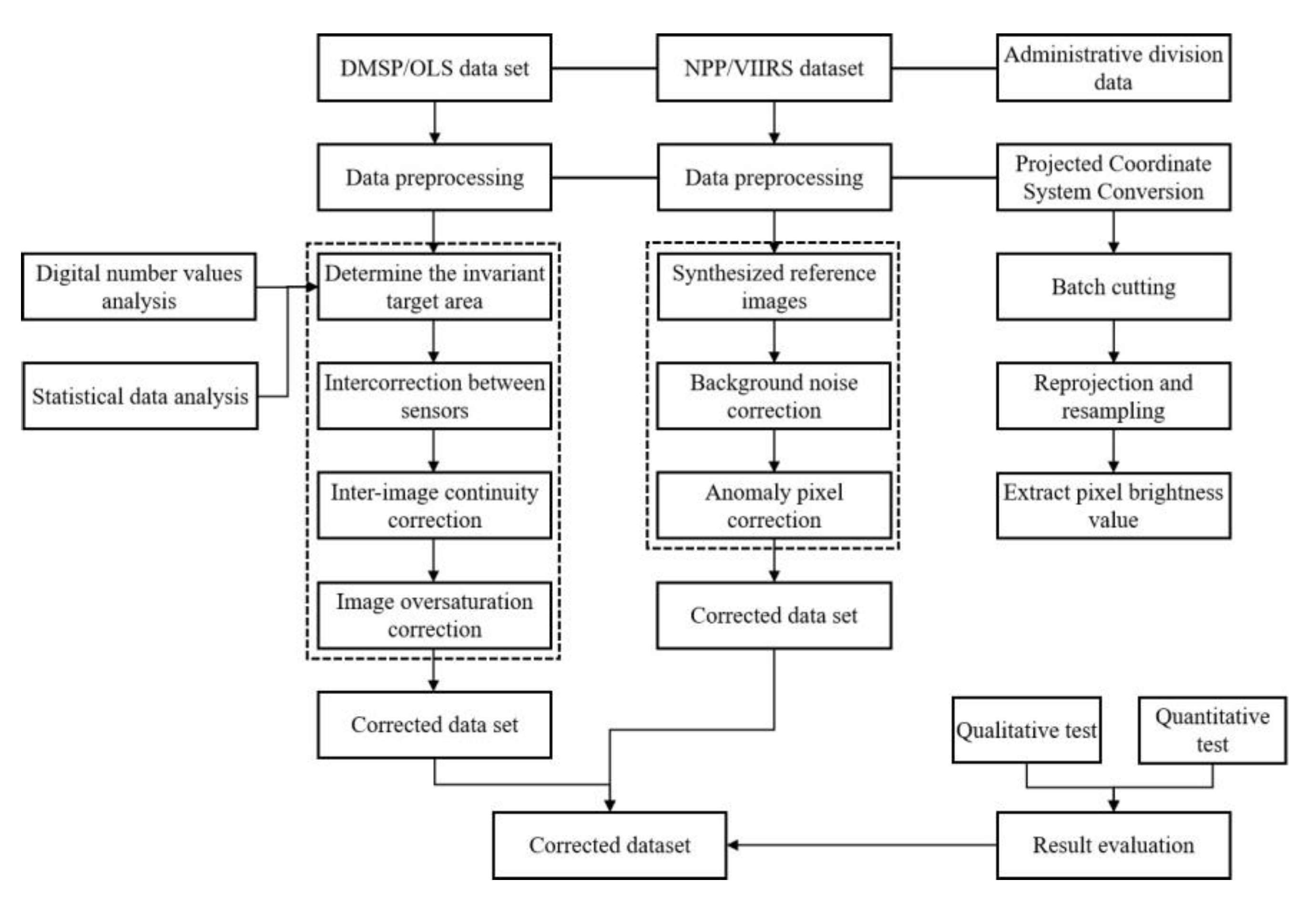
2.2.3. Night-Time Light Data

This research used night-time light data as a “ruler” to measure the spatial vitality of complex ecosystems, including DMSP/OLS and NPP/VIIRS images. Among them, DMSP/OLS selected the fourth edition of non radiation calibration night-time light data, and NPP/VIIRS selected vcm and vcm-orm-ntl types as monthly and annual data, respectively. Considering the serious distortion of night-time light data in the middle and high latitudes of China in the summer, the data from spring (April), autumn (September), and winter (December) are combined as the composite annual data. The annual night-time light data of 2015 and 2016 provided by the NOAA/NGDC website are set as the standard annual data [48,49]. After obtaining two kinds of night-time light data, it was necessary to preprocess and further correct them (Figure 2).

For DMSP/OLS data, Hegang City, Heilongjiang Province, with relatively stable economic development and a small change in night-time light intensity, is selected as the unchanged area. Firstly, the F16 sensor with a high DN value is selected as the standard sensor, and a monadic quadratic regression equation is established to calibrate the data of the other sensors. Secondly, the mean value is used to calibrate the data set after mutual correction between different sensors in the same year. Finally, based on the night-time light data of 2013, the DN values from 1993 to 2013 are dynamically adjusted by using a raster calculator [50,51].

$$\mathrm{M}\mathrm{u}\mathrm{t}\mathrm{u}\mathrm{a}\mathrm{l}\mathrm{c}\mathrm{o}\mathrm{r}\mathrm{r}\mathrm{e}\mathrm{c}\mathrm{t}\mathrm{i}\mathrm{o}\mathrm{n}\mathrm{b}\mathrm{e}\mathrm{t}\mathrm{w}\mathrm{e}\mathrm{e}\mathrm{n}\mathrm{d}\mathrm{i}\mathrm{f}\mathrm{f}\mathrm{e}\mathrm{r}\mathrm{e}\mathrm{n}\mathrm{t}\mathrm{s}\mathrm{e}\mathrm{n}\mathrm{s}\mathrm{o}\mathrm{r}\mathrm{s}:{\mathrm{D}\mathrm{N}}^{\prime }=\mathrm{a}\times {\mathrm{D}\mathrm{N}}^2+\mathrm{b}\times \mathrm{D}\mathrm{N}+\mathrm{c}$$

(1)

$$\mathrm{C}\mathrm{o}\mathrm{n}\mathrm{t}\mathrm{i}\mathrm{n}\mathrm{u}\mathrm{i}\mathrm{t}\mathrm{y}\mathrm{c}\mathrm{o}\mathrm{r}\mathrm{r}\mathrm{e}\mathrm{c}\mathrm{t}\mathrm{i}\mathrm{o}\mathrm{n}\mathrm{b}\mathrm{e}\mathrm{t}\mathrm{w}\mathrm{e}\mathrm{e}\mathrm{n}\mathrm{d}\mathrm{i}\mathrm{f}\mathrm{f}\mathrm{e}\mathrm{r}\mathrm{e}\mathrm{n}\mathrm{t}\mathrm{s}\mathrm{e}\mathrm{n}\mathrm{s}\mathrm{o}\mathrm{r}\mathrm{s}:{\mathrm{D}\mathrm{N}}_{\mathrm{n}}=\frac{{\mathrm{D}\mathrm{N}}_{\mathrm{n}}^{\mathrm{a}}+{\mathrm{D}\mathrm{N}}_{\mathrm{n}}^{\mathrm{b}}}{2}$$

(2)

$$\mathrm{Continuity}\mathrm{Correction}\mathrm{of}\mathrm{Time}\mathrm{Series}:\begin{array}{c}{\mathrm{D}\mathrm{N}}_{\left(\mathrm{n},\mathrm{i}\right)}=\left\{\begin{array}{cc}{\mathrm{D}\mathrm{N}}_{\left(\mathrm{n}-1,\mathrm{i}\right)}\hfill & {\mathrm{D}\mathrm{N}}_{\left(\mathrm{n}-1,,\mathrm{i}\right)}>{\mathrm{D}\mathrm{N}}_{\left(\mathrm{n},\mathrm{i}\right)}\hfill \\ {\mathrm{D}\mathrm{N}}_{\left(\mathrm{n},\mathrm{i}\right)}\hfill & \mathrm{Other}\hfill \end{array}\right.\hfill \\ (\mathrm{n}=1993,\dots ,2012,2013)\hfill \end{array}$$

(3)

In the formula, DN’ and DN represent a digital number after and before correction, respectively; a and b represent regression coefficients of the pixel gray value; and c is a constant term. ${\mathrm{D}\mathrm{N}}_{\mathrm{n}}^{\mathrm{a}}$ and ${\mathrm{D}\mathrm{N}}_{\mathrm{n}}^{\mathrm{b}}$ represent the n-th year DN value acquired with the a and b sensors, respectively; and ${\mathrm{D}\mathrm{N}}_{\mathrm{n}}$ represents the n-th year DN value after correction. ${\mathrm{D}\mathrm{N}}_{(\mathrm{n},\mathrm{i})}$ and ${\mathrm{D}\mathrm{N}}_{(\mathrm{n}-1,\mathrm{i})}$ represent the DN value of night-time light at i position in the n-th and n-1-th year, respectively. In order to keep the corrected DN value of night-time light data consistent with the original DN value range, the grid with the corrected DN value greater than 63 is assigned as 63.

There is no light saturation effect in NPP/VIIRS data, but there are a lot of weak lights, abnormally high values, and negative values, so it is necessary to reduce the standard deviation of the spatial distribution of DN values [52] as follows: Firstly, take the comprehensive annual data from 2015 as the benchmark data, and replace the negative value in the benchmark data with the standard annual data from 2015 provided by the website. Secondly, the DMSP/OLS night-time light of the coincident years of 2012 and 2013 are binarized, and the light and non-light areas are assigned as 1 and 0, respectively. Finally, the NPP/VIIRS data is simulated as the spatial variation characteristics of DMSP/OLS data using the logarithmic transformation data processing method [53].

$$\mathrm{N}\mathrm{e}\mathrm{g}\mathrm{a}\mathrm{t}\mathrm{i}\mathrm{v}\mathrm{e}\mathrm{n}\mathrm{u}\mathrm{m}\mathrm{b}\mathrm{e}\mathrm{r}\mathrm{e}\mathrm{l}\mathrm{i}\mathrm{m}\mathrm{i}\mathrm{n}\mathrm{a}\mathrm{t}\mathrm{i}\mathrm{o}\mathrm{n}:{\mathrm{D}\mathrm{N}}_{\mathrm{i}}=\left\{\begin{array}{cc}{\mathrm{D}\mathrm{N}}_{\mathrm{i}}\hfill & {\mathrm{D}\mathrm{N}}_{\mathrm{i}}\ge 0\hfill \\ {\mathrm{D}\mathrm{N}}_{2015}\hfill & {\mathrm{D}\mathrm{N}}_{\mathrm{i}}<0\hfill \end{array}\right.$$

(4)

$$\mathrm{L}\mathrm{o}\mathrm{g}\mathrm{a}\mathrm{r}\mathrm{i}\mathrm{t}\mathrm{h}\mathrm{m}\mathrm{i}\mathrm{c}\mathrm{t}\mathrm{r}\mathrm{a}\mathrm{n}\mathrm{s}\mathrm{f}\mathrm{o}\mathrm{r}\mathrm{m}\mathrm{a}\mathrm{t}\mathrm{i}\mathrm{o}\mathrm{n}:{\log }_{\_}{\mathrm{N}\mathrm{P}\mathrm{P}}_{\mathrm{x},\mathrm{y}}=\ln \left({\mathrm{N}\mathrm{P}\mathrm{P}}_{\mathrm{x},\mathrm{y}}+1\right)$$

(5)

In the formula, ${\mathrm{D}\mathrm{N}}_{\mathrm{i}}$ represents the grid value of the 2015 composite annual data, and ${\mathrm{D}\mathrm{N}}_{2015}$ represents the grid value of the 2015 standard annual data. By analogy, taking the composite annual data from 2015 as the benchmark data, the negative values in the composite annual data from 2012 to 2014 are replaced with the non-negative values in the data from the following year, and the negative values in the synthetic annual data from 2016 to 2019 are replaced with the non-negative values in the data from the previous year, so as to obtain the composite annual night-time light data without negative values.

DMSP/OLS and NPP/VIIRS both contain night-time light data in 2012 and 2013, and the spatial distribution characteristics of DN values are similar. Assuming that DMSP/OLS continues to update after 2013, a functional relationship can be established with NPP/VIIRS data from the same year as follows. Considering the saturation effect of the DMSP/OLS data, take the DN value range of 0~50 as the mask, and construct five fitting models, including the logarithm, quadratic polynomial, linear, exponential, and power function. Finally, the 2013 quadratic polynomial model with the best results was selected to correct the NPP/VIIRS data from 2012 to 2020.

$$\mathrm{Q}\mathrm{u}\mathrm{a}\mathrm{d}\mathrm{r}\mathrm{a}\mathrm{t}\mathrm{i}\mathrm{c}\mathrm{p}\mathrm{o}\mathrm{l}\mathrm{y}\mathrm{n}\mathrm{o}\mathrm{m}\mathrm{i}\mathrm{a}\mathrm{l}\mathrm{m}\mathrm{o}\mathrm{d}\mathrm{e}\mathrm{l}:\mathrm{D}=0.2352{\mathrm{N}}^2+21.932\mathrm{N}-2.8764$$

(6)

In the formula, N is the DN value of the original NPP/VIIRS data, and D is the DN value of the simulated DMSP/OLS data.

Since there is still a small amount of weak light in the simulated NPP/VIIRS data, a 5 × 5 Gaussian low-pass filtering operation can be performed using ENVI 5.3 software to achieve the purpose of noise reduction [54], and the grid with a DN value greater than 63 in the simulated NPP/VIIRS data is assigned a value of 63. Finally, this paper constructs the night-time light data set of Lixiahe Plain from 1992 to 2020.

2.3. Measurement Method of Spatial Vitality Factors of Complex Ecosystem

2.3.1. Economic, Social, and Natural Subsystems

In order to extract the spatial vitality factors of the economic, social, and natural subsystems of the Lixiahe River Plain, Pearson’s correlation analysis, multiple stepwise regression analysis, and multiple fitting analysis were conducted between the pixel value (DN value) and the pixels number (Count value) of the night-time light data and the economic, social, and natural subsystem elements, respectively, by using SPSS 23.0 software. Following these analyses, the interdependence between the spatial vitality factors in the region was obtained.

Firstly, the POI data of the economic and social subsystem elements and land use/cover data of the natural subsystem elements in Lixiahe Plain were imported into Arc GIS software to create a grid (fishing net) with a pixel width and height of 1 × 1 km. Secondly, the spatial grid processing is carried out, and the spatial grid whose pixel value is 0 is eliminated to get the pixel number and pixel value of the spatial grid of different subsystem elements. Thirdly, the night-time light data at the same spatial scale are extracted using the spatial grid as the mask, and Pearson’s correlation analysis and a single sample Kolmogorov–Smirnov test are performed. Finally, the multiple regression equation between the accumulated value of night-time light and the pixel number and the pixel value of economic, social, and natural subsystem elements is established, and 11 spatial vitality factors of the economic, social, and natural subsystems in Lixiahe Plain are screened.

2.3.2. Population Subsystems

The existing research has proved that there is a significant correlation between the accumulated value of night-time light data and the population data, but the correlation between different spatial scales and different regions is quite different [55]. Firstly, this paper conducts a pre-test on the statistical population and the accumulated value of night-time light at the township scale and measures the regression coefficient and intercept of the regression model. The result shows that the quadratic polynomial regression model in the polynomial regression has the best curve-fitting degree. Secondly, the simulated value of the population (POP’) of each night-time light pixel (grid) in Lixiahe Plain is calculated. Finally, the population calibration parameter Kn is used to calibrate and obtain the final simulated value of the population (Grid Pop), which is equal to the statistical value of the population of each township unit [56,57].

$$\mathrm{T}\mathrm{o}\mathrm{w}\mathrm{n}\mathrm{s}\mathrm{h}\mathrm{i}\mathrm{p}\mathrm{s}\mathrm{c}\mathrm{a}\mathrm{l}\mathrm{e}\mathrm{p}\mathrm{o}\mathrm{p}\mathrm{u}\mathrm{l}\mathrm{a}\mathrm{t}\mathrm{i}\mathrm{o}\mathrm{n}\mathrm{s}\mathrm{i}\mathrm{m}\mathrm{u}\mathrm{l}\mathrm{a}\mathrm{t}\mathrm{i}\mathrm{o}\mathrm{n}:{\mathrm{P}\mathrm{O}\mathrm{P}}_{\mathrm{n}}=0.0009{{\mathrm{T}\mathrm{D}\mathrm{N}}_{\mathrm{n}}}^2+33.181{\mathrm{T}\mathrm{D}\mathrm{N}}_{\mathrm{n}}+2133.9$$

(7)

$$\mathrm{G}\mathrm{r}\mathrm{i}\mathrm{d}\mathrm{s}\mathrm{c}\mathrm{a}\mathrm{l}\mathrm{e}\mathrm{p}\mathrm{o}\mathrm{p}\mathrm{u}\mathrm{l}\mathrm{a}\mathrm{t}\mathrm{i}\mathrm{o}\mathrm{n}\mathrm{s}\mathrm{i}\mathrm{m}\mathrm{u}\mathrm{l}\mathrm{a}\mathrm{t}\mathrm{i}\mathrm{o}\mathrm{n}:{\mathrm{P}\mathrm{O}\mathrm{P}}_{\mathrm{i}}^{\prime }=0.0009{{\mathrm{T}\mathrm{D}\mathrm{N}}_{\mathrm{i}}}^2+33.181\mathrm{T}\mathrm{D}\mathrm{N}+\frac{2133.9}{{\mathrm{T}\mathrm{D}\mathrm{N}}_{\mathrm{i}}}$$

(8)

$$\mathrm{G}\mathrm{r}\mathrm{i}\mathrm{d}\mathrm{s}\mathrm{c}\mathrm{a}\mathrm{l}\mathrm{e}\mathrm{p}\mathrm{o}\mathrm{p}\mathrm{u}\mathrm{l}\mathrm{a}\mathrm{t}\mathrm{i}\mathrm{o}\mathrm{n}\mathrm{c}\mathrm{a}\mathrm{l}\mathrm{i}\mathrm{b}\mathrm{r}\mathrm{a}\mathrm{t}\mathrm{i}\mathrm{o}\mathrm{n}:{\mathrm{G}\mathrm{r}\mathrm{i}\mathrm{d}\mathrm{P}\mathrm{o}\mathrm{p}}_{\mathrm{i}}={\mathrm{P}\mathrm{O}\mathrm{P}}_{\mathrm{i}}^{\prime }\times {\mathrm{K}}_{\mathrm{n}}={\mathrm{P}\mathrm{O}\mathrm{P}}_{\mathrm{i}}^{\prime }\times \frac{{\mathrm{T}\mathrm{P}\mathrm{P}}_{\mathrm{n}}}{{\mathrm{T}\mathrm{M}\mathrm{P}}_{\mathrm{n}}}$$

(9)

In the formula, ${\mathrm{P}\mathrm{O}\mathrm{P}}_{\mathrm{n}}$ represents the simulated value of the population of the n-th township in Lixiahe Plain. ${\mathrm{T}\mathrm{D}\mathrm{N}}_{\mathrm{n}}$ refers to the accumulated night-time light value of the n-th township. ${\mathrm{P}\mathrm{O}\mathrm{P}}_{\mathrm{i}}^{\prime }$ represents the simulated value of the population of the i-th night-time light pixel, and ${\mathrm{T}\mathrm{D}\mathrm{N}}_{\mathrm{i}}$ represents the accumulated night-time light value of the i-th night-time light pixel. ${\mathrm{G}\mathrm{r}\mathrm{i}\mathrm{d}\mathrm{P}\mathrm{o}\mathrm{p}}_{\mathrm{i}}$ is the simulated value of the population of the i-th night-time light pixel after correction, and the corrected proportional parameter (K_n) is the ratio of the statistical value of the population (TPP_n) to the initial simulation value of the population (TMP_n).

In order to verify the accuracy of the population distribution in grid scale, this paper uses the relative error between the statistical value of the population and the simulated value of the population to test the accuracy [58].

$$\mathrm{C}\mathrm{a}\mathrm{l}\mathrm{c}\mathrm{u}\mathrm{l}\mathrm{a}\mathrm{t}\mathrm{i}\mathrm{o}\mathrm{n}\mathrm{o}\mathrm{f}\mathrm{r}\mathrm{e}\mathrm{l}\mathrm{a}\mathrm{t}\mathrm{i}\mathrm{v}\mathrm{e}\mathrm{e}\mathrm{r}\mathrm{r}\mathrm{o}\mathrm{r}:\mathrm{R}\mathrm{E}=\frac{{\mathrm{P}\mathrm{O}\mathrm{P}}_{\mathrm{i}}^{\prime }-{\mathrm{P}\mathrm{O}\mathrm{P}}_{\mathrm{i}}}{{\mathrm{P}\mathrm{O}\mathrm{P}}_{\mathrm{i}}}$$

(10)

In the formula, RE is relative error, ${\mathrm{P}\mathrm{O}\mathrm{P}}_{\mathrm{i}}$ is the statistical value of the population of the i-th township unit, and ${\mathrm{P}\mathrm{O}\mathrm{P}}_{\mathrm{i}}^{\prime }$ is the simulated value of the population of the i-th township unit.

Calculate the residual value of the statistical value of the population and the simulated value of the population based on Formula (9), divide the residual value into 9 segments and use different functions to correct them, respectively, and set the negative value of the corrected population as 0 (

Table 1. Residual correction method of the simulated value of the population based on night-time light data.

Residual	Correction Function	Corrected R2	Corrected RMSE
(−∞,−81,000]	y = 1.6886x + 77,699	0.9899	5251
[−80,999,−51,000]	y = 1.0341x + 63,274	0.9962	4192
[−50,999,−21,000]	y = 1.0380x + 32,621	0.9789	8515
[−20,999,−6000]	y = 1.0091x + 11,757	0.9607	4352
[−5999,5999]	y = 0.9735x + 764	0.9799	3173
[6000,20,999]	y = 0.9831x − 11,748	0.9740	3911
[21,000,50,999]	y = 0.9675x − 28,749	0.9740	7956
[51,000,80,999]	y = 0.9772x − 58,297	0.9885	7565
[81,000,+∞)	y = 0.9064x − 87,002	0.9999	547

).

Firstly, the subsection correction function used by different township units is determined, and then the intercept value in each subsection function is divided by the number of night-time light pixels in the township unit where the grid is located.

$$\mathrm{R}\mathrm{e}\mathrm{v}\mathrm{i}\mathrm{s}\mathrm{i}\mathrm{o}\mathrm{n}\mathrm{o}\mathrm{f}\mathrm{p}\mathrm{o}\mathrm{p}\mathrm{u}\mathrm{l}\mathrm{a}\mathrm{t}\mathrm{i}\mathrm{o}\mathrm{n}\mathrm{g}\mathrm{r}\mathrm{i}\mathrm{d}\mathrm{r}\mathrm{e}\mathrm{s}\mathrm{u}\mathrm{l}\mathrm{t}\mathrm{s}:{{\mathrm{P}\mathrm{O}\mathrm{P}}_{\mathrm{i}}^{″}=\mathsf{\alpha }\times \mathrm{G}\mathrm{r}\mathrm{i}\mathrm{d}\mathrm{P}\mathrm{o}\mathrm{p}}_{\mathrm{i}}+\mathsf{\beta }/\mathsf{\gamma }$$

(11)

In the formula, ${\mathrm{P}\mathrm{O}\mathrm{P}}_{\mathrm{i}}^{\prime \prime }$ is the simulated value of population of the i-th night-time light pixel corrected using ${\mathrm{G}\mathrm{r}\mathrm{i}\mathrm{d}\mathrm{P}\mathrm{o}\mathrm{p}}_{\mathrm{i}}$. $\mathsf{\alpha }$ and $\mathsf{\beta }$ respectively represent the scale coefficient and intercept of the subsection function used for the i-th night-time light pixel, respectively.

After correction, the variation range of residual was narrowed from [−116,137,125,130] to [−18,025,19,008]. The accuracy of the spatial population estimation was significantly improved, and the data shortcomings of the OLS sensor were effectively corrected.

2.4. Evaluation Method of Spatial Vitality of Complex Ecosystem

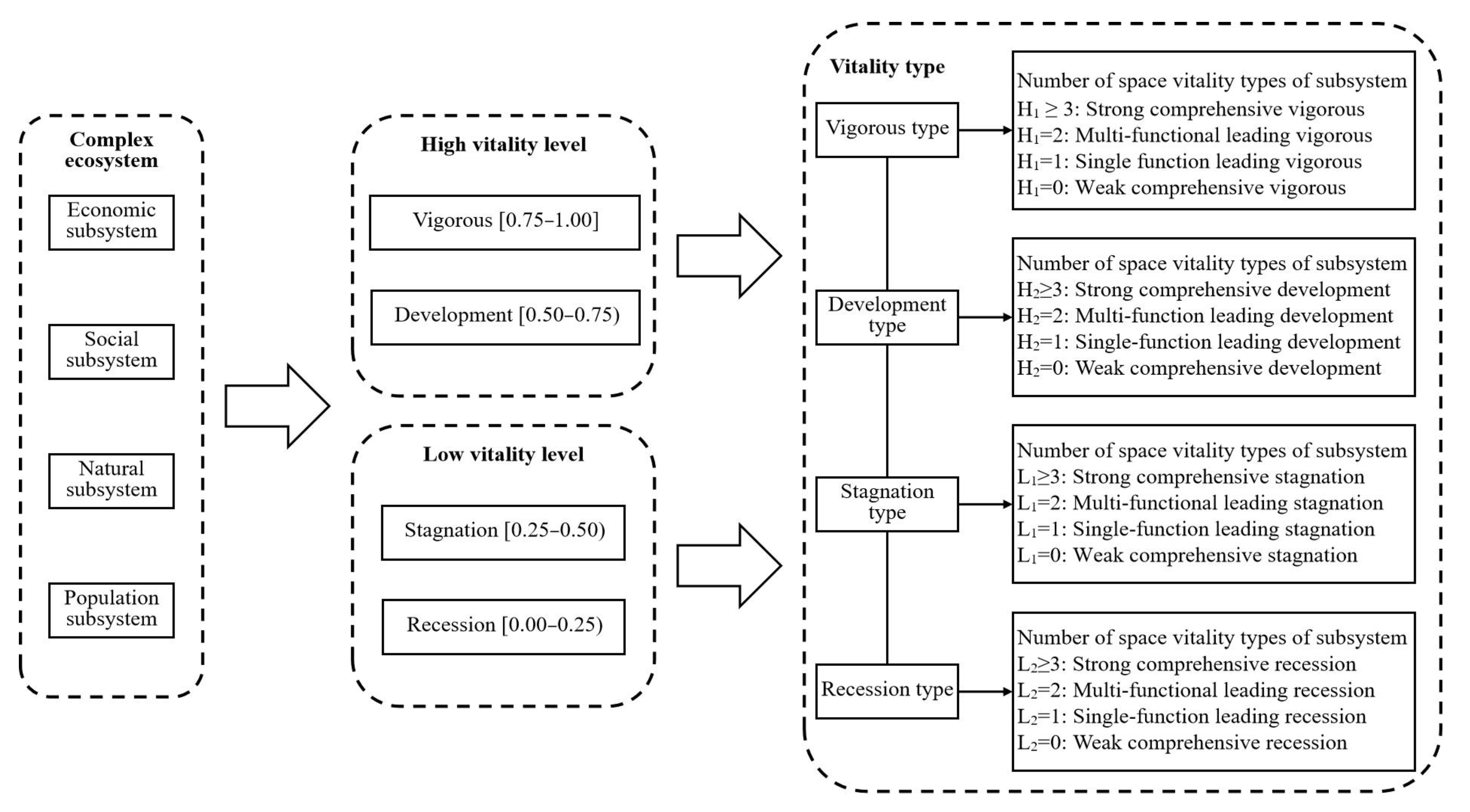
2.4.1. Assessment Framework

The complex ecosystem in this study includes the economic subsystem (ES), social subsystem (SS), natural subsystem (NS), and population subsystem (PS). According to the measurement results of spatial vitality factors, the actual research situation in the study area, the relevant articles on spatial vitality indices, and the opinions of 15 experts, the 12 categories of indices are further subdivided and expanded into 29 indices. The analytic hierarchy process (AHP) and the entropy weight method (EWM) were comprehensively used to calculate the subjective and objective weights of the indices of the spatial vitality assessment framework of the complex ecosystem in Lixiahe Plain [59,60,61]. Then, the weight distribution was more reasonable using the normalization method of multiplication synthesis (

Table 2. Assessment framework, weights, and reference values of the complex ecosystem in Lixiahe region.

Subsystem	NO.	Indices	Unit	Reference	AHP	EWM	Comprehensive	Features
Economic	X1	Hotel	Pixel	4.54 c	0.145	0.068	0.016	+
	X2	Inn	Pixel	3.47 c	0.174	0.031	0.009	+
	X3	Bank, ATM	Pixel	3.36 c	0.136	0.104	0.023	+
	X4	Insurance, Securities, Finance	Pixel	3.15 c	0.148	0.045	0.012	+
	X5	Company	Pixel	24.69 c	0.104	0.160	0.028	+
	X6	Factory	Pixel	9.14 c	0.149	0.241	0.060	+
	X7	GDP per km2	Million yuan/km2	0.96 a	0.143	0.352	0.084	+
Social	X8	Entertainment and leisure place	Pixel	5.63 c	0.102	0.044	0.008	+
	X9	Stadium	Pixel	2.29 c	0.254	0.090	0.038	+
	X10	General and specialized hospitals	Pixel	4.35 c	0.105	0.090	0.016	+
	X11	Clinics and health center	Pixel	6.07 c	0.098	0.031	0.005	+
	X12	Airport and railway station	Pixel	0.90 c	0.214	0.189	0.067	+
	X13	Subway and bus station	Pixel	17.41 c	0.096	0.189	0.030	+
	X14	Accessibility of public services	/	1.62 c	0.132	0.366	0.080	+
Natural	X15	Cultivated land	Pixel	52.21 c	0.026	0.074	0.003	+
	X16	Grassland	Pixel	0.48 c	0.279	0.125	0.058	+
	X17	Water area	Pixel	8.65 c	0.086	0.074	0.011	+
	X18	Urban construction land	Pixel	3.91 c	0.079	0.340	0.044	+
	X19	Rural residential area	Pixel	6.40 c	0.032	0.191	0.010	+
	X20	Other construction land	Pixel	0.32 c	0.190	0.120	0.038	+
	X21	Unused land	Pixel	0.03 c	0.273	0.045	0.020	+
	X22	Ecosystem service value	10 thousand yuan/km2	397 b	0.035	0.030	0.002	+
Population	X23	Population	10 thousand persons	6.85 a	0.287	0.110	0.053	+
	X24	Natural population growth rate	‰	0.17 a	0.148	0.562	0.138	+
	X25	Average years of education	year	10.21 a	0.305	0.069	0.035	+
	X26	Proportion of labor force population	%	62.95 a	0.260	0.258	0.112	+

Notes: ^a Jiangsu Province average value, ^b National average value, ^c Lixiahe Plain average value. The benchmark values of various indices are derived from the statistical yearbooks, environmental bulletins and measured data of the country, Jiangsu Province and Lixiahe Plain.

).

2.4.2. Evaluation Model

The calculation of the spatial vitality value of the composite ecosystem should refer to the benchmark value of each index. In order to ensure the correctness and effectiveness of the evaluation, the benchmark value of each index is mainly determined according to the national or local recognized value, the optimal value, or the average value.

$$\mathrm{P}\mathrm{o}\mathrm{s}\mathrm{i}\mathrm{t}\mathrm{i}\mathrm{v}\mathrm{e}\mathrm{i}\mathrm{n}\mathrm{d}\mathrm{i}\mathrm{c}\mathrm{e}\mathrm{s}:{\mathrm{x}}_{\mathrm{i}}\ge {\mathrm{y}}_{\mathrm{i}},{\mathrm{S}}_{\mathrm{i}}=1;{\mathrm{x}}_{\mathrm{i}}<{\mathrm{y}}_{\mathrm{i}},{\mathrm{S}}_{\mathrm{i}}={\mathrm{x}}_{\mathrm{i}}/{\mathrm{y}}_{\mathrm{i}}$$

(12)

$$\mathrm{N}\mathrm{e}\mathrm{g}\mathrm{a}\mathrm{t}\mathrm{i}\mathrm{v}\mathrm{e}\mathrm{i}\mathrm{n}\mathrm{d}\mathrm{i}\mathrm{c}\mathrm{e}\mathrm{s}:{\mathrm{x}}_{\mathrm{i}}\le {\mathrm{y}}_{\mathrm{i}},{\mathrm{S}}_{\mathrm{i}}=1;{\mathrm{x}}_{\mathrm{i}}>{\mathrm{y}}_{\mathrm{i}},{\mathrm{S}}_{\mathrm{i}}={\mathrm{y}}_{\mathrm{i}}/{\mathrm{x}}_{\mathrm{i}}$$

(13)

In the formula, S_i is the spatial vitality value of each index of the complex ecosystem. x_i is the actual value of each index, and y_i is the reference value of each index.

According to the spatial vitality indices and their corresponding weights in the assessment framework for spatial vitality of the complex ecosystem in Lixiahe Plain, the comprehensive index weighting method was used to calculate the spatial vitality value of each subsystem and the complex ecosystem, and the evaluation model of spatial vitality of the complex ecosystem in Lixiahe Plain was established.

$$\begin{gathered} \mathrm{ES}={\sum }_{\mathrm{i}=\mathrm{p}}^{\mathrm{q}}{\mathrm{W}}_{\mathrm{i}}\times {\mathrm{S}}_{\mathrm{i}},\mathrm{SS}={\sum }_{\mathrm{i}=\mathrm{p}}^{\mathrm{q}}{\mathrm{W}}_{\mathrm{i}}\times {\mathrm{S}}_{\mathrm{i}} \\ \mathrm{NS}={\sum }_{\mathrm{i}=\mathrm{p}}^{\mathrm{q}}{\mathrm{W}}_{\mathrm{i}}\times {\mathrm{S}}_{\mathrm{i}},\mathrm{PS}={\sum }_{\mathrm{i}=\mathrm{p}}^{\mathrm{q}}{\mathrm{W}}_{\mathrm{i}}\times {\mathrm{S}}_{\mathrm{i}} \end{gathered}$$

(14)

$$\mathrm{CE}=\mathrm{ES}+\mathrm{SS}+\mathrm{NS}+\mathrm{PS}$$

(15)

In the formula, ES, SS, NS, PS, and CE represent the spatial vitality values of the economic subsystem, social subsystem, natural subsystem, population subsystem and complex ecosystem in Lixiahe Plain, respectively.

2.4.3. Division of Rank

In order to ensure a scientific and reasonable division of the spatial vitality value and the level of the complex ecosystem in Lixiahe Plain, in this paper, the data standardization method was adopted to standardize the spatial vitality values of the four subsystems within the range of [0,1]. Then, this paper defines [0.00–0.25), [0.25–0.50), [0.50–0.75) and [0.75–1.00] as four levels of vigorous, development, stagnation, and recession, respectively.

$$\mathrm{V}=\frac{{\mathrm{V}}_{\mathrm{i}\mathrm{j}}-{\mathrm{V}}_{\mathrm{m}\mathrm{i}\mathrm{n}}}{{\mathrm{V}}_{\mathrm{m}\mathrm{a}\mathrm{x}}-{\mathrm{V}}_{\mathrm{m}\mathrm{i}\mathrm{n}}}$$

(16)

In the formula, there are values for the subsystem of the i-th township unit. V_ij is the actual spatial vitality value of the j-th subsystem of the i-th township unit. V_min and V_max are the lowest and highest values of spatial vitality of the subsystem, respectively.

2.4.4. Type Identification

Due to the differences in the spatial vitality levels of subsystems of different township spatial units, when the spatial vitality levels of a certain subsystem of a township occupy a dominant position, the subsystem plays a decisive role in the development of the township, while other subsystems are in a subordinate position.

$${\mathrm{C}}_{\mathrm{j}}={\mathrm{D}}_{\mathrm{i}\mathrm{j}}-\frac{{\mathrm{D}}_{\mathrm{j}}}{\mathrm{n}}$$

(17)

In the formula, C_j represents the difference between the spatial vitality value of the j-th subsystem of the i-th township unit (D_ij) and the average value of the j-th subsystem (D_j/n).

When the number of advantage subsystems of the “vigorous type” is 0, it is defined as a weak comprehensive type. When the number of advantage subsystems of the “vigorous type” is 1, it is defined as a single-function leading type. When the number of advantage subsystems of the “vigorous type” is 2, it is defined as a multi-functional leading type. When the number of advantage subsystems of the “vigorous type” is 3 or 4, it is defined as a strong comprehensive type. In addition, the division principle of the spatial vitality level of the development, stagnation, and recession type is the same as that of the vigorous type (Figure 3).

2.5. Coupling Coordination Method of Spatial Vitality of the Complex Ecosystem

2.5.1. Coupling Degree Model

In this paper, the quantitative research of coupling degree draws on the capacitive coupling coefficient model in physics. The coupling degree is high when the subsystems are promoted by each other. On the contrary, the coupling degree is low when the subsystems are mutually restraint by each other [62,63].

$$\mathrm{O}\mathrm{r}\mathrm{d}\mathrm{e}\mathrm{r}\mathrm{p}\mathrm{a}\mathrm{r}\mathrm{a}\mathrm{m}\mathrm{e}\mathrm{t}\mathrm{e}\mathrm{r}:{\mathrm{U}}_{\mathrm{i}}=\sum {\mathrm{\lambda }}_{\mathrm{i}}{\mathrm{u}}_{\mathrm{i}\mathrm{j}}(0\le {\mathrm{\lambda }}_{\mathrm{i}},\sum {\mathrm{\lambda }}_{\mathrm{i}}=1)$$

(18)

$$\mathrm{C}\mathrm{o}\mathrm{u}\mathrm{p}\mathrm{l}\mathrm{i}\mathrm{n}\mathrm{g}\mathrm{d}\mathrm{e}\mathrm{g}\mathrm{r}\mathrm{e}\mathrm{e}\mathrm{m}\mathrm{o}\mathrm{d}\mathrm{e}\mathrm{l}:\mathrm{C}={\left[\frac{{\mathrm{U}}_1{\mathrm{U}}_2{\mathrm{U}}_3{\mathrm{U}}_4}{{\left(\frac{{\mathrm{U}}_1+{\mathrm{U}}_2+{\mathrm{U}}_3+{\mathrm{U}}_4}{\mathrm{n}}\right)}^{\mathrm{n}}}\right]}^{\mathrm{k}}(\mathrm{k}\ge 2)$$

(19)

In the formula, ${\mathrm{U}}_{\mathrm{I}}$ is the order parameter of the coupling system ${\mathrm{\lambda }}_{\mathrm{I}}$ is the weight of each order parameter. ${\mathrm{u}}_{\mathrm{i}\mathrm{j}}$ represents the spatial vitality value of the i-th subsystem of the j-th township unit. j∈{1, 2, 3... 359} represents the 359 township units in Lixiahe Plain. C is the coupling degree of the vitality space of the complex ecosystem, and its value ranges from 0 to 1. n∈{1, 2, 3..., 4} represents the number of subsystems. k is the adjustment coefficient, and its value is n. U₁, U₂, U₃, and U₄ are the spatial vitality values of the economic, social, natural, and population subsystems, respectively.

The coupling degree of Lixiahe Plain is divided into three types by using the natural breakpoint classification (NBC) based on the existing research results and the actual situation of this study (

Table 3. Classification of coupling degree.

Type	Features
Low coupling	The subsystems mutual games with each other, showing low coupling characteristics
General coupling	The subsystems interaction with each other, showing general coupling characteristics
High coupling	The subsystems cooperate with each other, showing a high coupling characteristics

).

2.5.2. Coupling Coordination Model

Because the coupling degree model can only show the degree of interaction among subsystems, it cannot reflect the level of coordinated development. Therefore, the coupling coordination degree model is introduced to reflect the coordination relationship among subsystems under different correlation effects.

$$\mathrm{D}\mathrm{e}\mathrm{v}\mathrm{e}\mathrm{l}\mathrm{o}\mathrm{p}\mathrm{m}\mathrm{e}\mathrm{n}\mathrm{t}\mathrm{m}\mathrm{o}\mathrm{d}\mathrm{e}\mathrm{l}:\mathrm{T}=\mathsf{\alpha }{\mathrm{U}}_1+\mathsf{\beta }{\mathrm{U}}_2+\mathsf{\gamma }{\mathrm{U}}_3+{\mathsf{\chi }\mathrm{U}}_4$$

(20)

$$\mathrm{C}\mathrm{o}\mathrm{u}\mathrm{p}\mathrm{l}\mathrm{i}\mathrm{n}\mathrm{g}\mathrm{c}\mathrm{o}\mathrm{o}\mathrm{r}\mathrm{d}\mathrm{i}\mathrm{n}\mathrm{a}\mathrm{t}\mathrm{i}\mathrm{o}\mathrm{n}\mathrm{m}\mathrm{o}\mathrm{d}\mathrm{e}\mathrm{l}:\mathrm{D}=\sqrt{\mathrm{C}\mathrm{T}}$$

(21)

In the formula, D is the coupling coordination degree of spatial vitality of the complex ecosystem, with a value range of 0–1. T is the comprehensive development index of the spatial vitality of the subsystem. α, β, γ, and χ are the undetermined coefficients of the spatial vitality of the economic, social, natural, and population subsystems, respectively, and the comprehensive weight values of each subsystem index in the above assessment framework were used, namely α = 0.232, β = 0.244, γ = 0.186, and χ = 0.338.

The coupling coordination degree of Lixiahe Plain is divided into three types by using the natural breakpoint classification (NBC) based on the existing research results and the actual situation of this study (

Table 4. Classification of the coupling coordination degree.

Type	Features
Recession maladjustment	The subsystems cannot promote each other, and there are serious mutual constraints or exclusions
Basic coordination	The subsystems are in a barely coordinated state, and the trend of mutual promotion is not obvious
Coordinated development	All subsystems develop coordinately and complement each other

).

2.5.3. Spatial Correlation Analysis

In order to accurately identify the distribution characteristics of spatial vitality of township units in Lixiahe Plain, the local Moran’s I was used to reveal the clustering characteristics and intensity of spatial vitality, and to find out the units or sub-regions with spatial agglomeration, namely, LISA (local indicators of spatial associations).

$$\mathrm{L}\mathrm{o}\mathrm{c}\mathrm{a}\mathrm{l}{\mathrm{M}\mathrm{o}\mathrm{r}\mathrm{a}\mathrm{n}}^{\prime }\mathrm{s}\mathrm{I}:{\mathrm{I}}_{\mathrm{i}}=\frac{{\mathrm{Z}}_{\mathrm{i}}}{{\mathrm{S}}^2}\sum _{\mathrm{j}\ne \mathrm{i}}^{\mathrm{n}}{\mathrm{W}}_{\mathrm{i}\mathrm{j}}{\mathrm{Z}}_{\mathrm{j}}$$

(22)

$$\mathrm{D}\mathrm{i}\mathrm{s}\mathrm{c}\mathrm{r}\mathrm{e}\mathrm{t}\mathrm{e}\mathrm{v}\mathrm{a}\mathrm{r}\mathrm{i}\mathrm{a}\mathrm{n}\mathrm{c}\mathrm{e}\mathrm{o}\mathrm{f}{\mathrm{y}}_{\mathrm{i}}:{\mathrm{S}}^2=\frac{1}{\mathrm{n}}\sum _{\mathrm{i}=1}^{\mathrm{n}}({\mathrm{y}}_{\mathrm{i}}-\overline{\mathrm{y}})$$

(23)

$$\mathrm{S}\mathrm{i}\mathrm{g}\mathrm{n}\mathrm{i}\mathrm{f}\mathrm{i}\mathrm{c}\mathrm{a}\mathrm{n}\mathrm{c}\mathrm{e}\mathrm{t}\mathrm{e}\mathrm{s}\mathrm{t}:\mathrm{Z}({\mathrm{I}}_{\mathrm{i}})=\frac{{\mathrm{I}}_{\mathrm{i}}-\mathrm{E}\left({\mathrm{I}}_{\mathrm{i}}\right)}{\sqrt{\mathrm{V}\mathrm{a}\mathrm{r}\left({\mathrm{I}}_{\mathrm{i}}\right)}}$$

(24)

In the formula,${\mathrm{I}}_{\mathrm{i}}$ is the local Moran’s I of the i-th township. S² is the discrete variance of y_i. n is the total number of samples, that is, the number of township units. W_ij is the spatial weight between township i and township j, where if the two spaces are adjacent, W_ij is taken as 1, and if not adjacent, W_ij is taken as 0. ${\mathrm{Z}}_{\mathrm{i}}$ and ${\mathrm{Z}}_{\mathrm{j}}$ represent the difference between the attribute value of township units i and j and the average value of the attribute of 359 township units in the region, respectively. Z (I_i) is the significance test formula of local Moran’s I.

Since local Moran’s I has no range limitation, when I_i > 0, it means that the attribute values of the i-th township unit are similar to those of adjacent units, and when I_i < 0, it means that the attribute values of this township unit are not similar to those of adjacent units (

Table 5. Four combinations of local Moran’s I.

$\mathbf{Bivariate}$		Local Moran’s I	Meaning
${\mathbf{Z}}_{\mathbf{i}}$	$\sum _{\mathbf{i}\ne \mathbf{j}}^{\mathbf{n}}{\mathbf{W}}_{\mathbf{i}\mathbf{j}}{\mathbf{Z}}_{\mathbf{j}}$	Ii
>0	>0	>0	The i-th region has a high level of development, and the surrounding areas have a high level of development
<0	<0	>0	The i-th region has a low level of development, and the surrounding areas have a low level of development
<0	>0	<0	The i-th region has a low level of development, and the surrounding areas have a high level of development
>0	<0	<0	The i-th region has a high level of development, and the surrounding areas have a low level of development

).

2.5.4. Exploratory Space–Time Data Analysis

In this paper, the exploratory spatio-temporal data analysis (ESTDA) method is used to analyze the evolution of the coupling coordination degree of each subsystem in time and space [64].

$$\mathrm{R}\mathrm{e}\mathrm{l}\mathrm{a}\mathrm{t}\mathrm{i}\mathrm{v}\mathrm{e}\mathrm{l}\mathrm{e}\mathrm{n}\mathrm{g}\mathrm{t}\mathrm{h}:{\mathrm{R}\mathrm{L}}_{\mathrm{i}}=\frac{\mathrm{n}\times \sum _{\mathrm{t}=1}^{\mathrm{T}-1}\mathrm{d}({\mathrm{L}}_{\mathrm{i},\mathrm{t}},{\mathrm{L}}_{\mathrm{i},\mathrm{t}+1})}{\sum _{\mathrm{i}=1}^{\mathrm{n}}\sum _{\mathrm{t}=1}^{\mathrm{T}-1}\mathrm{d}({\mathrm{L}}_{\mathrm{i},\mathrm{t}},{\mathrm{L}}_{\mathrm{i},\mathrm{t}+1})}$$

(25)

$$\mathrm{C}\mathrm{u}\mathrm{r}\mathrm{v}\mathrm{a}\mathrm{t}\mathrm{u}\mathrm{r}\mathrm{e}:{\mathrm{D}}_{\mathrm{i}}=\frac{\sum _{\mathrm{t}=1}^{\mathrm{T}-1}\mathrm{d}({\mathrm{L}}_{\mathrm{i},\mathrm{t}},{\mathrm{L}}_{\mathrm{i},\mathrm{t}+1})}{\mathrm{d}({\mathrm{L}}_{\mathrm{i},\mathrm{t}},{\mathrm{L}}_{\mathrm{i},\mathrm{T}})}$$

(26)

In the formula, ${\mathrm{R}\mathrm{L}}_{\mathrm{i}}$ is the relative length. n represents the number of township units. T is the research time series, T∈{1,2,3,...,t}$.{\mathrm{L}}_{\mathrm{i},\mathrm{t}}$ and ${\mathrm{L}}_{\mathrm{i},\mathrm{t}+1}$ represent the positions of a township unit i in Moran’s I scatterplot in year t and year t + 1, respectively. d (L_i,t, L_i,t+1) is the distance that township unit i moves from year t to year t + 1. D_i is the bending degree.

LISA’s space–time transition method is used to measure the transition state of the spatial correlation types of the coupling degree and coupling coordination degree, which are divided into four types (

Table 6. Types of spatial-temporal transitions.

Type	Form	Symbol
Type I	Self transition and neighborhood stability	HH→LH; HL→LL; LH→HH; LL→HL
Type Ⅱ	Self stability and neighborhood transition	HH→HL; HL→HH; LH→LL; LL→LH
Type Ⅲ	Both self and neighborhood transitions	HH→LL; HL→LH; LH→HL; LL→HH
Type Ⅳ	Both self and neighborhood stability	HH→HH; HL→HL; LH→LH; LL→LL

).

3. Results and Analysis

3.1. Spatial Vitality Evaluation of Complex Ecosystem

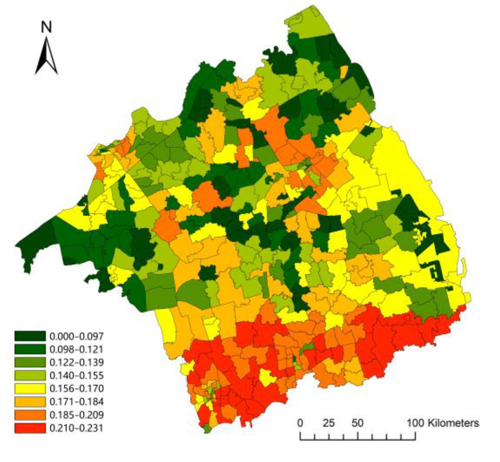
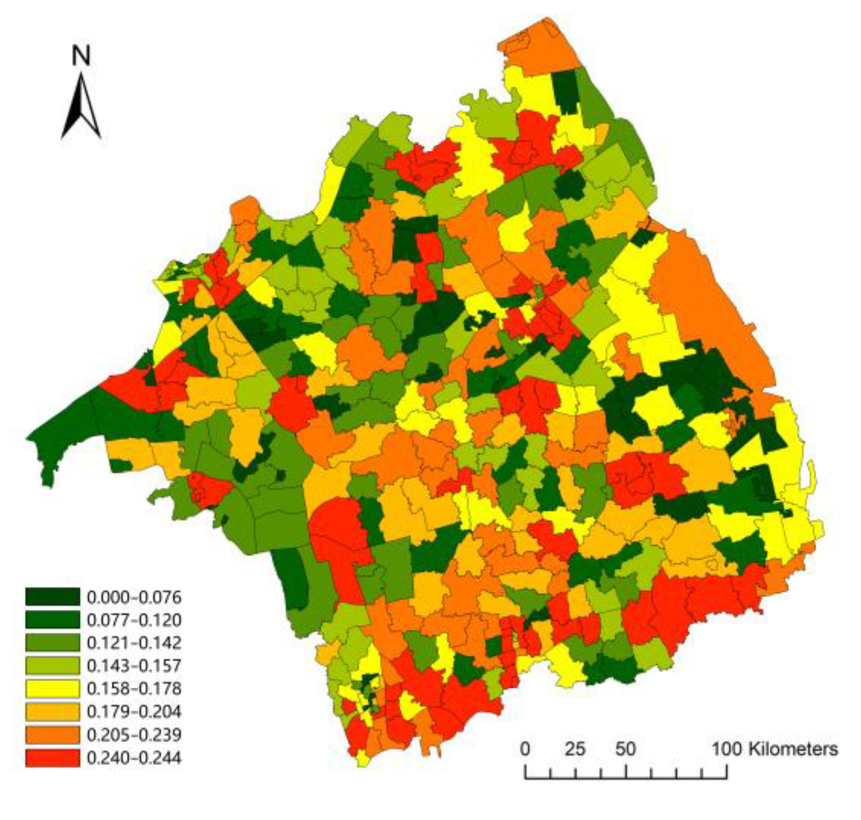
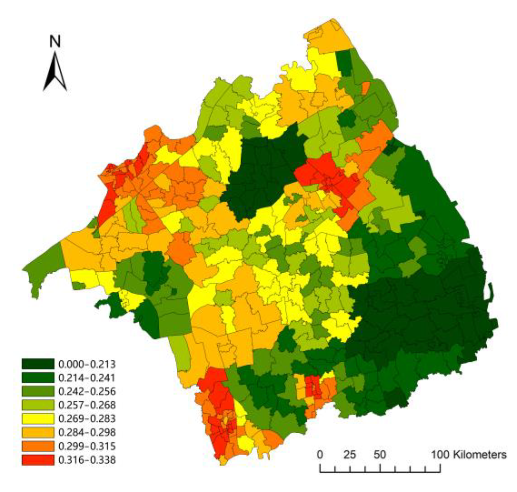
3.1.1. Gradient Characteristics of the Spatial Vitality of the Complex Ecosystem

The spatial vitality value of the complex ecosystem in Lixiahe Plain is between 0.265 and 0.916, with an average value of 0.639. About 36.18% of the township unit scores are in the high range of [0.7–1.0), and about 58.89% of the township unit scores are in the median range of [0.4–0.7). This shows that the spatial vitality of the complex ecosystem is good, but there are great differences between regions (Figure 4). Among them, the average value of the spatial vitality of the economic subsystem is 0.152, and the spatial vitality is general. The minimum and maximum values are located in the county units of Jinhu County and Guangling District, respectively (Figure 5). The average value of the spatial vitality of the social subsystem is 0.158, and each index value is significantly lower than the average value of Jiangsu Province. The minimum and maximum values are located in 19 county units such as Dafeng District and Baoying County, respectively (Figure 6). The average value of the spatial vitality of the natural subsystem is 0.063, and the spatial vitality is poor. The process of resource development and urban–rural construction is not synchronized. The ecological environment of township units with better urban and rural construction is more general, and the urban and rural construction of township units with a better ecological environment is more general. The minimum and maximum values are located in the county units of Funing County and Jiangdu District, respectively (Figure 7). The average value of the spatial vitality of the population subsystem is 0.266, and the spatial vitality is good. The minimum and maximum values are located in the county units of Dongtai City, Hanjiang District, and Qingjiangpu District, respectively (Figure 8).

From the perspective of the spatial vitality gradient characteristics, the spatial vitality value of the complex ecosystem in Lixiahe Plain fluctuated downward from west to east. The spatial vitality values of the economic subsystems are ranked from high to low as 0.160 in the western region, 0.147 in the central region, and 0.145 in the eastern region. Among them, the number of spatial units with the vigorous type and the development type of economic subsystems in the western region accounted for 49.5% and 43.7% of the total number of regional township units, respectively. The number of spatial units with the stagnation type of economic subsystems in the central region accounted for 46.7% of the total number of regional township units. The number of spatial units with the recession type of economic subsystems in the eastern region accounted for 47.1% of the total number of regional township units. This is basically consistent with the fluctuation of the spatial vitality value change curve of the economic subsystem.

The spatial vitality values of the social subsystems are ranked from high to low as 0.160 in the central region, 0.159 in the western region, and 0.151 in the eastern region. The number of spatial units with the vigorous type, development type, and stagnation type of social subsystems in the western and central regions accounted for 76.6%, 77.4%, and 77.6% of the total number of regional township units, respectively. The number of spatial units with the recession type of social subsystems in the eastern region accounted for 47.1% of the total number of regional township units. Regional conditions and road traffic facilities have become important factors affecting the spatial vitality of social subsystems.

The spatial vitality values of natural subsystems are ranked from high to low as 0.067 in the western region, 0.063 in the eastern region, and 0.058 in the central region. The number of spatial units with the vigorous type and stagnation type of natural subsystems in the western region accounted for 75.0% and 52.3% of the total number of regional township units, respectively. The number of spatial units with the development type of natural subsystems in the eastern region accounted for 44.1% of the total number of regional township units. The number of spatial units with the recession type of natural subsystems in the central region accounted for 41.2% of the total number of regional township units. This shows that the favorable natural environment will affect the site selection and construction of the urban and rural areas to some extent and enhance the spatial vitality.

The spatial vitality values of the population subsystems are ranked from high to low as 0.289 in the western region, 0.256 in the central region, and 0.243 in the eastern region. The number of spatial units with the vigorous type and development type of population subsystems in the western region and central region accounted for 72.0% and 52.5% of the total number of regional township units, respectively. The number of spatial units with the stagnation type and recession type of population subsystems in the eastern region accounted for 44.4% and 60.7% of the total number of regional township units, respectively. This shows that the gradient characteristic of the spatial vitality value of the population subsystem in Lixiahe Plain is significant (Figure 9 and Figure 10).

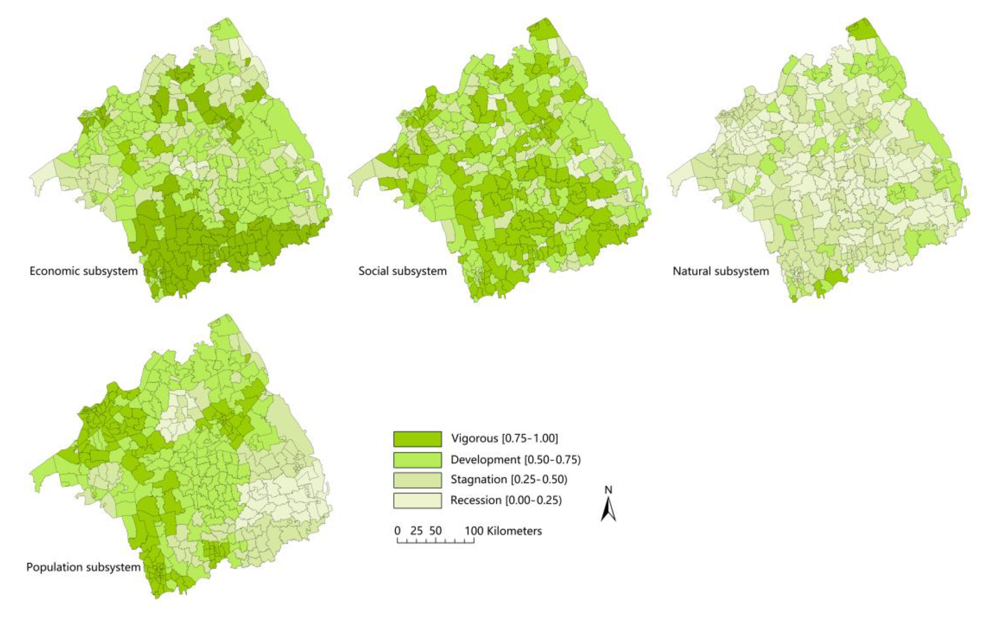
3.1.2. Distribution Characteristics of Spatial Vitality of Complex Ecosystem

The spatial vitality level of the economic subsystem has good local consistency. The number of township units at the vigorous level accounts for 5.59%, with an average value of more than 0.180, which is mainly distributed in six county units in the south, including Guangling, Hanjiang, Jiangdu, etc. The number of township units at the recession level accounts for 30.26%, with an average value of less than 0.075, which is mainly distributed in six county units in the south, including Sheyan, Dafeng, Dongtai, etc.

The spatial vitality level of the social subsystems shows obvious gradient distribution characteristics, and the vigorous level of township units is mainly distributed in the areas of water and land transportation, such as the 24 township units under the jurisdiction of Jiangdu, Gaoyou, Baoying, and other county units along the lines of Beijing-Hangzhou Canal, G2 Expressway, G233 National Highway, etc. However, most of the township units in the recession level are far away from the traffic trunk lines.

The township units with a vigorous level of spatial vitality of the natural subsystem are mainly distributed in the Jiajiang River of the Yangtze River, the mouth of the main irrigation canal in northern Jiangsu Province, and the location between the Jing-Hang Canal and the Yangtze River channel, such as Lidian Town of Guangling District, etc. The development level is mainly distributed in the township units with a prominent natural landscape in the main urban area of each county unit. However, the recession level of the township units is mostly manifested in the asynchrony between urban and rural construction and ecological environment development.

The spatial vitality level of the population subsystem has good local consistency. Most of the vigorous township units are distributed in the western region, accounting for 23.68% of the total. For example, the spatial vitality values of seven county units, including Qingjiangpu, Huai’an, and Hongze, are above 0.293. The township units with the recession level of spatial vitality of the population subsystem are mainly distributed in the north central and southeast, accounting for about 8.88%. For example, the spatial vitality values of Dongtai and Jianhu county units are below 0.195 (Figure 11).

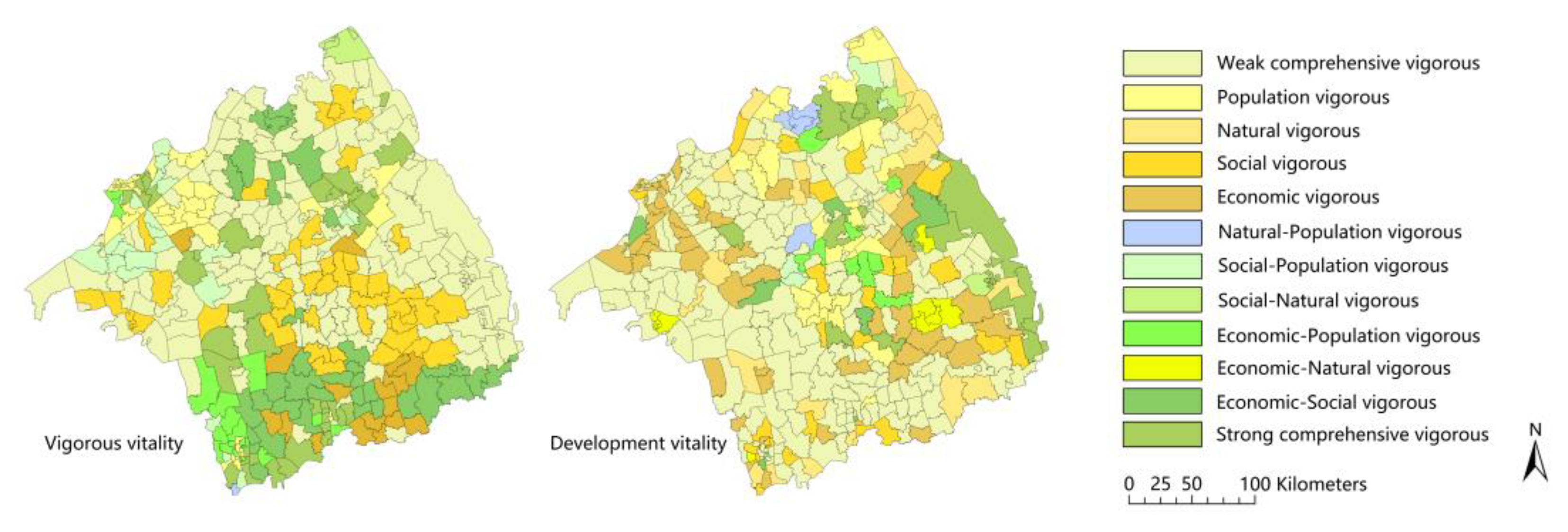
3.1.3. Type Distribution of the Spatial Vitality of the Complex Ecosystem

According to the identification rules of spatial vitality types of a complex ecosystem, the different spatial vitality types of the 359 township units in the 20 county units of Lixiahe Plain can be classified into 25 types. This includes four major types: vigorous, development, stagnation, and recession. Each major type is further divided into four middle types: strong comprehensive, multi-functional leading, single-function leading, and weak comprehensive. Each middle type is further divided into six subtypes: economy–society leading, economy–nature leading, economy–population leading, society–nature leading, society–population leading, and natural–population leading (

Table 7. Type and quantity statistics of the spatial vitality complex ecosystem in Lixiahe region.

Level	Type			Quantity
	Major	Middle	Sub	Major	Middle	Sub
High vitality level	Vigorous type	Strong comprehensive vigorous type	/	359	39	39
		Multi-functional leading vigorous type	Economic–social vigorous type		80	35
			Economic–population vigorous type			18
			Social–natural vigorous type			1
			Social–population vigorous type			25
			Natural–population vigorous type			1
		Single-function leading vigorous type	Economic vigorous type		107	17
			Social vigorous type			41
			Population vigorous type			49
		Weak comprehensive vigorous type	/		133	133
	Development type	Strong comprehensive development type	/	359	12	12
		Multi-functional leading development type	Economic–social development type		34	8
			Economic–natural development type			9
			Economy–population development type			8
			Social–natural development type			2
			Social–population development type			4
			Natural–population development type			3
		Single-function leading development type	Economic development type		128	52
			Social development type			29
			Natural development type			22
			Population development type			25
		Weak comprehensive development type	/		185	185
Low vitality level	Stagnation type	Single-function leading stagnation type	Natural stagnation type	359	138	138
		Weak comprehensive stagnation type	/		221	221
	Recession type	Weak comprehensive recession type	/	359	359	359

).

The strong comprehensive vigorous type of vitality space was distributed in 39 township units under the jurisdiction of 9 county units, and the comprehensive score was between 0.733 and 0.916. Among them, the number of county units in Huaian, Guangling, and Baoying in the western regions was the largest, followed by Hailing and Tinghu in the central and eastern regions. The multi-functional leading vigorous type of vitality space was widely distributed in 80 township units under the jurisdiction of 17 county units, and most of them were economic–social leading type, economic–population leading type, and social–population leading type. It shows the distribution characteristics of high spatial vitality of the economic subsystem in the south, high spatial vitality of the population subsystem in the west, and high spatial vitality of the social subsystem in the north. The single-function leading vigorous type of vitality space had the widest distribution, including 107 township units under 19 county units. The economic vigorous type was mainly distributed in 6 county units, including Jiangyan, Hai’an, and Jiangdu, the social vigorous type was mainly distributed in 10 county space units, including Dongtai, Xinghua, and Sheyang, and the population vigorous type was mainly distributed in 8 county units, including Qingjiangpu, Huai’an, and Hanjiang.

The strong comprehensive development type of vitality space was distributed in 11 township units under the jurisdiction of 6 county units, and the comprehensive score was between 0.639 and 0.806. Among them, the number of county units in Sheyang, Dafeng, and Dongtai in eastern regions was the largest, followed by Yandu and Xinghua in the central and Baoying in the western regions. The multi-functional leading development vitality type of vitality space was distributed in 34 township units under the jurisdiction of 13 county units, and most of them were concentrated. The multi-functional leading development type of the vitality space was distributed in 34 township units under the jurisdiction of 13 county units, and most of them were concentrated in the middle of the central and eastern regions, which had obvious spatial differentiation characteristics with the vigorous type of vitality space. For example, the multi-functional leading vigorous type of vitality space has local consistency characteristics, while the multi-functional leading development type vitality space presents the interleaved spatial distribution characteristics. The single-function leading development type of vitality space has the widest spatial distribution, including 128 township units under the jurisdiction of 20 county units. Among them, the number and distribution of the economic development type of vitality space were the largest, followed by the number of the population development type of vitality space, but the distribution concentration was the strongest (Figure 12).

3.2. Coupling Regulation Mechanism of the Complex Ecosystem

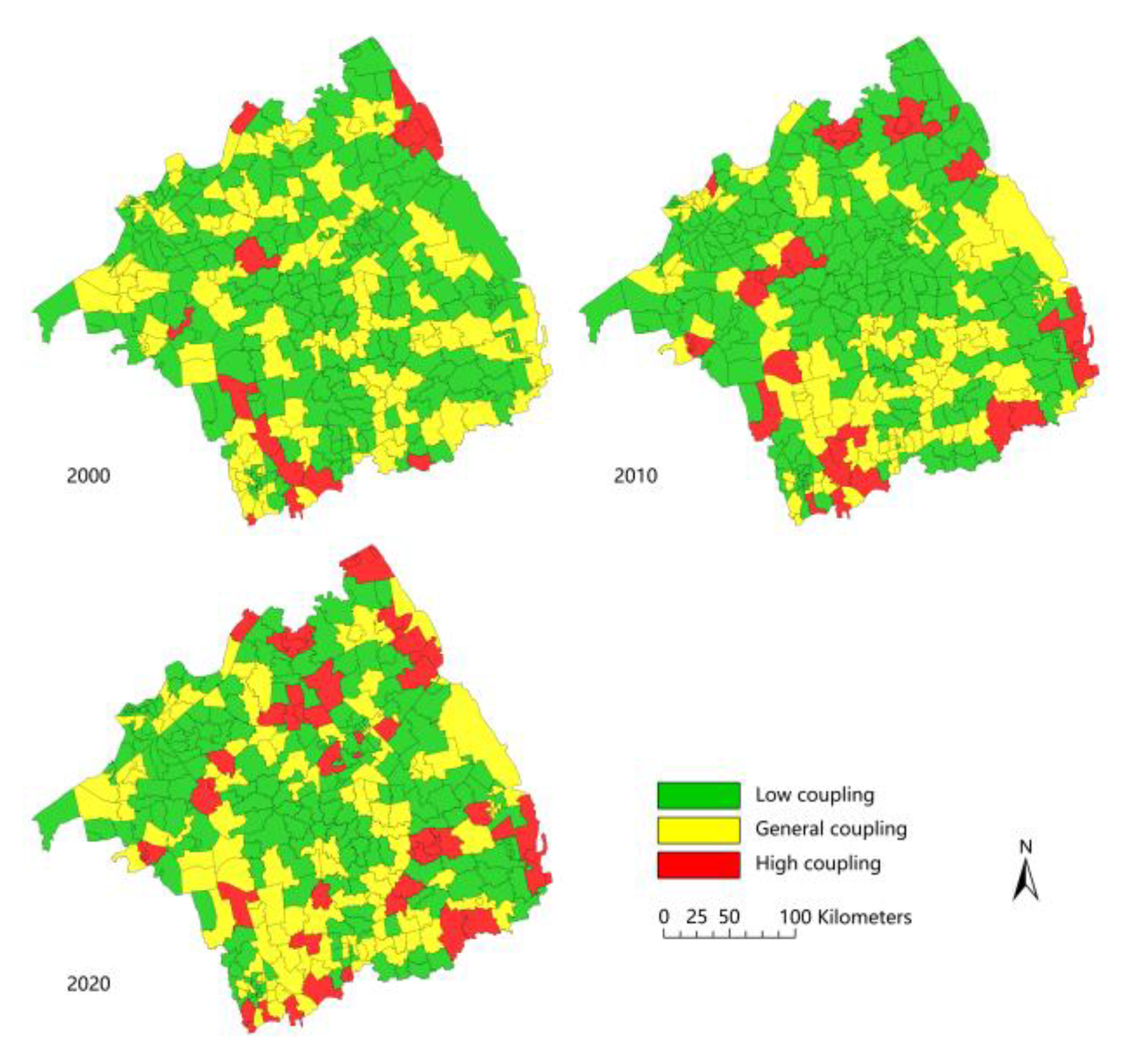
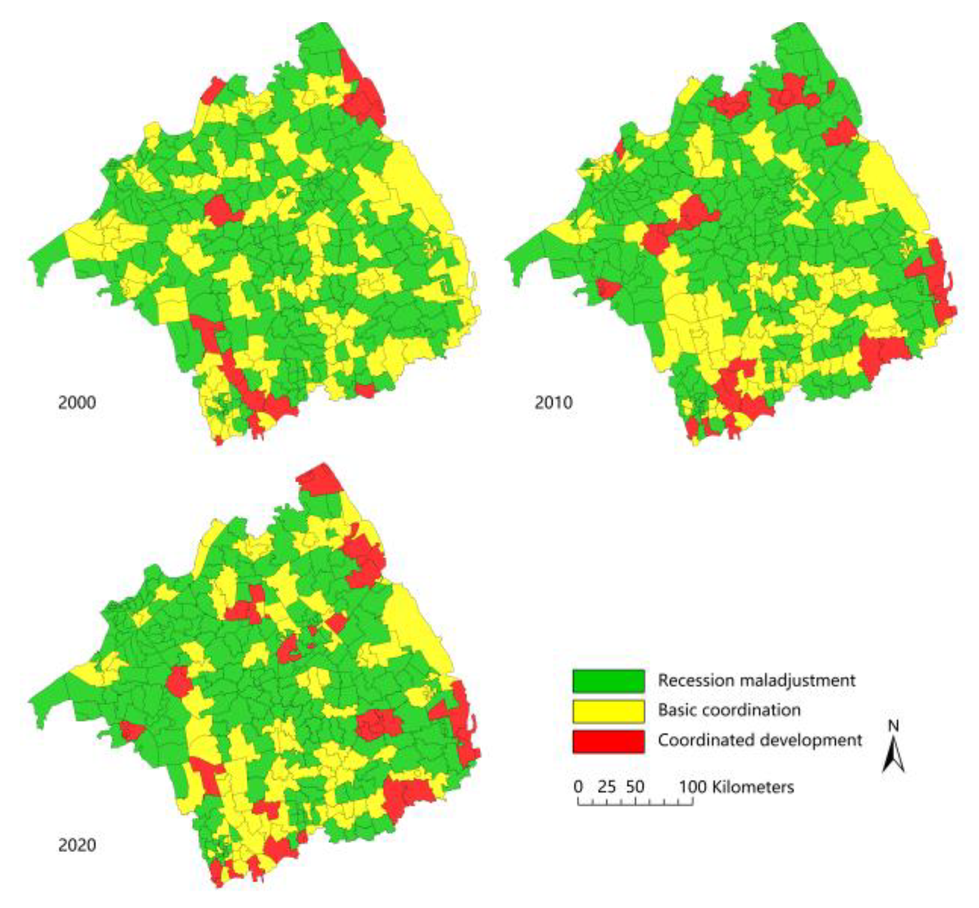
3.2.1. Spatial-Temporal Evolution Analysis of Coupling Coordination of Spatial Vitality of the Complex Ecosystem

From 2000 to 2020, the number of township units with high coupling degree and high coupling coordination degree showed a gradual growth trend, from 13 to 12 in 2000, from 23 to 22 in 2010, and then from 40 to 30 in 2020. Among them, the average values in 2000 were 0.762 and 0.060, respectively, which were highly overlapping in spatial distribution, mainly concentrated in the suburban towns of county units with a good water ecological environment. The average values in 2010 were 0.888 and 0.079, respectively, which were highly overlapping in spatial distribution, and both spread to surrounding towns and streets with Chengguan Town (the residence of the county government) as the center. The average values in 2020 were 0.876 and 0.070, respectively, the number of township units in the latter was significantly less than that in the former, and the difference was mainly shown in the township units in the suburbs and the outer suburbs. Although the mean values of high coupling degree and high coupling co-scheduling have decreased, the number of high coupling degree township units has increased significantly.

From 2000 to 2020, the number of township units with a low coupling degree and a low coupling coordination degree showed a trend of increasing first and then decreasing, and decreasing first and then increasing, respectively. The number of township units with a low coupling degree increased from 126 in 2000 to 222 in 2010, and then the number decreased to 196 in 2020. The number of township units with a low coupling coordination degree decreased from 238 in 2000 to 236 in 2010, and then the number increased to 239 in 2020. It can be found that from 2000 to 2020, the spatial vitality of the low coupling degree and low coupling coordination degree of township units in Lixiahe Plain gradually converged from the decentralized distribution to the central and northern regions.

Among them, the north–south difference in the number of township units with low coupling degree and low coupling coordinated degree was enlarged from 2000 to 2010. From 2000 to 2010, the north–south difference in the number of township units with a low coupling degree and a low coupling coordinated degree was enlarged. From 2010 to 2020, the quantity difference between the north and the south of township units with a low coupling degree decreased gradually, while the quantity difference between the north and the south of township units with a low coupling degree did not alleviate (Figure 13 and Figure 14).

The overlap degree of coupling degree and coupling coordination degree in “high-high” type areas is higher. Although the number of coupling coordination degrees in “high-high” type areas is less than that of the coupling degree, it also shows a rising trend year by year. Among them, the aggregation area shifted from the southwest and northeast in 2000 to the southwest and northwest in 2010, and then clustered in the southwest, south central, southeast, and northeast in 2020. The distribution of the “high-high” type area of the coupling degree in the southern region was greatly affected by the spatial vitality type of the natural subsystem, while the northern region was jointly affected by the spatial vitality level and type. When the spatial vitality level of natural subsystems in the southern region was significantly improved, or the difference of the spatial activity level in the northern region decreased, the region showed an obvious “high-high” type distribution.

The overlap degree of the coupling degree and coupling coordination degree in “low-low” type areas is higher. Both of them show significant aggregation distribution characteristics, and are concentrated in the central and northern regions, but the number of township units in the latter is significantly less than the former. Among them, from 2000 to 2010, the number of “low-low” type areas with a coupling degree increased significantly, but the coupling coordination degree generally decreased, and the benign effect between township units was weakened. From 2010 to 2020, the number of low-low type areas in the central region decreased significantly, while the number of low-low type areas in the northern region increased significantly, indicating that the spatial vitality level in the central region increased significantly in recent years, and the influence degree among township units increased to a certain extent. Although the spatial vitality level and type of the economic, social, and population subsystems in the northern region are good, the coordinated development value among the subsystems is low, and the ability of mutual promotion is weak.

The number of “high-low” type areas of coupling degree and coordination degree was the least, and they were greatly affected by the spatial distribution of “low-low” type areas, mainly around the “low-low” type areas in the north. From 2000 to 2010, there was only Yangzhai Town in Funing County in the north. From 2010 to 2020, it was distributed in Huaicheng Town of Huai ‘an City in the north, Panwan Town of Sheyang County in the northeast, and Qinnan Town of Yandu District in the middle. The spatial distribution of the coupling degree and coupling coordination degree of the “low-high” type area was completely consistent, which was greatly affected by the spatial distribution of the “high-high” type areas, mainly around the “high-high” type areas in the north. In 2000, the type areas were mostly distributed in the southeastern county units. In 2100, the number of type areas in the east and north increased, and in 2020, the number of type areas in the southeast increased (Figure 15 and Figure 16).

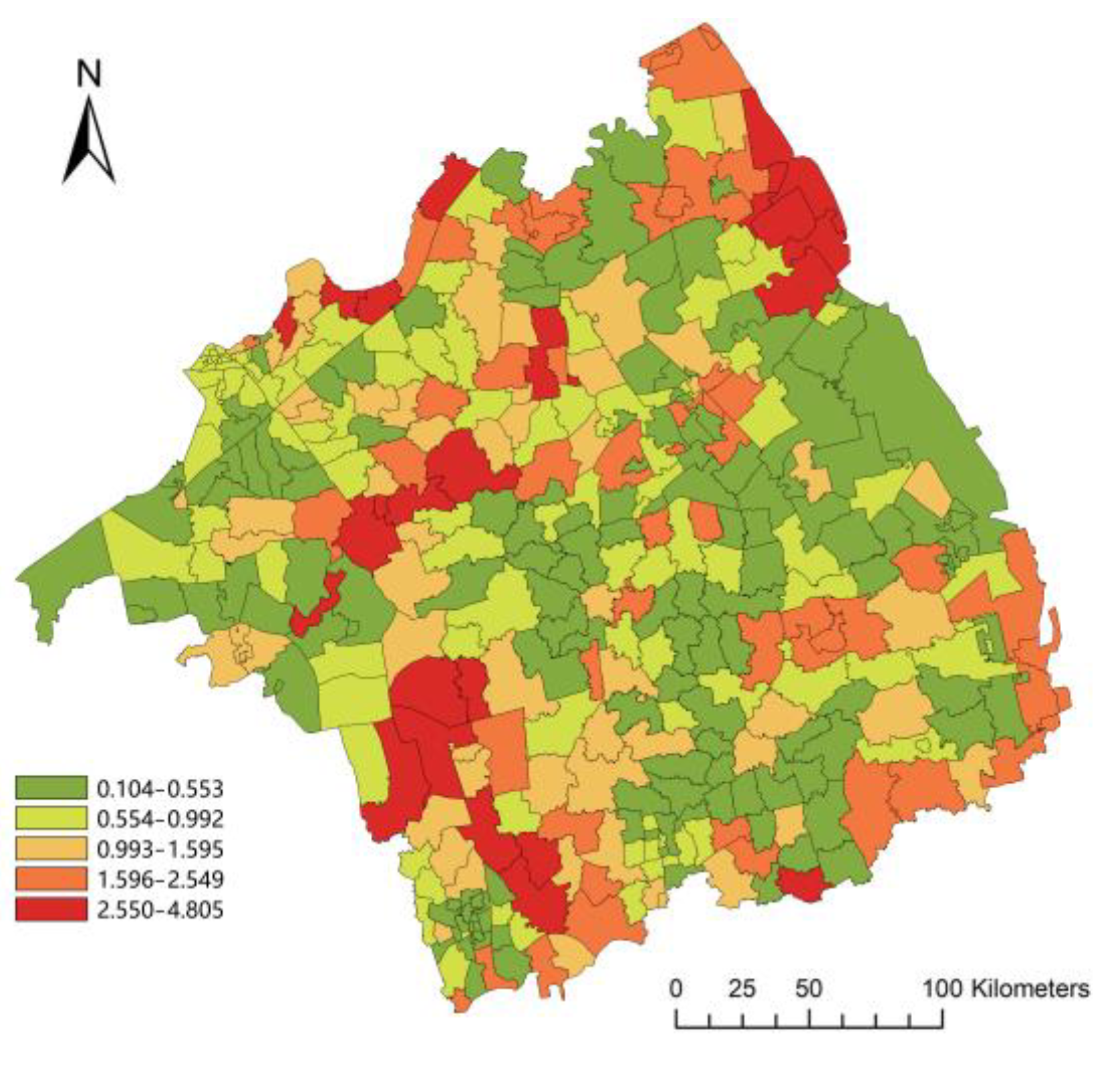
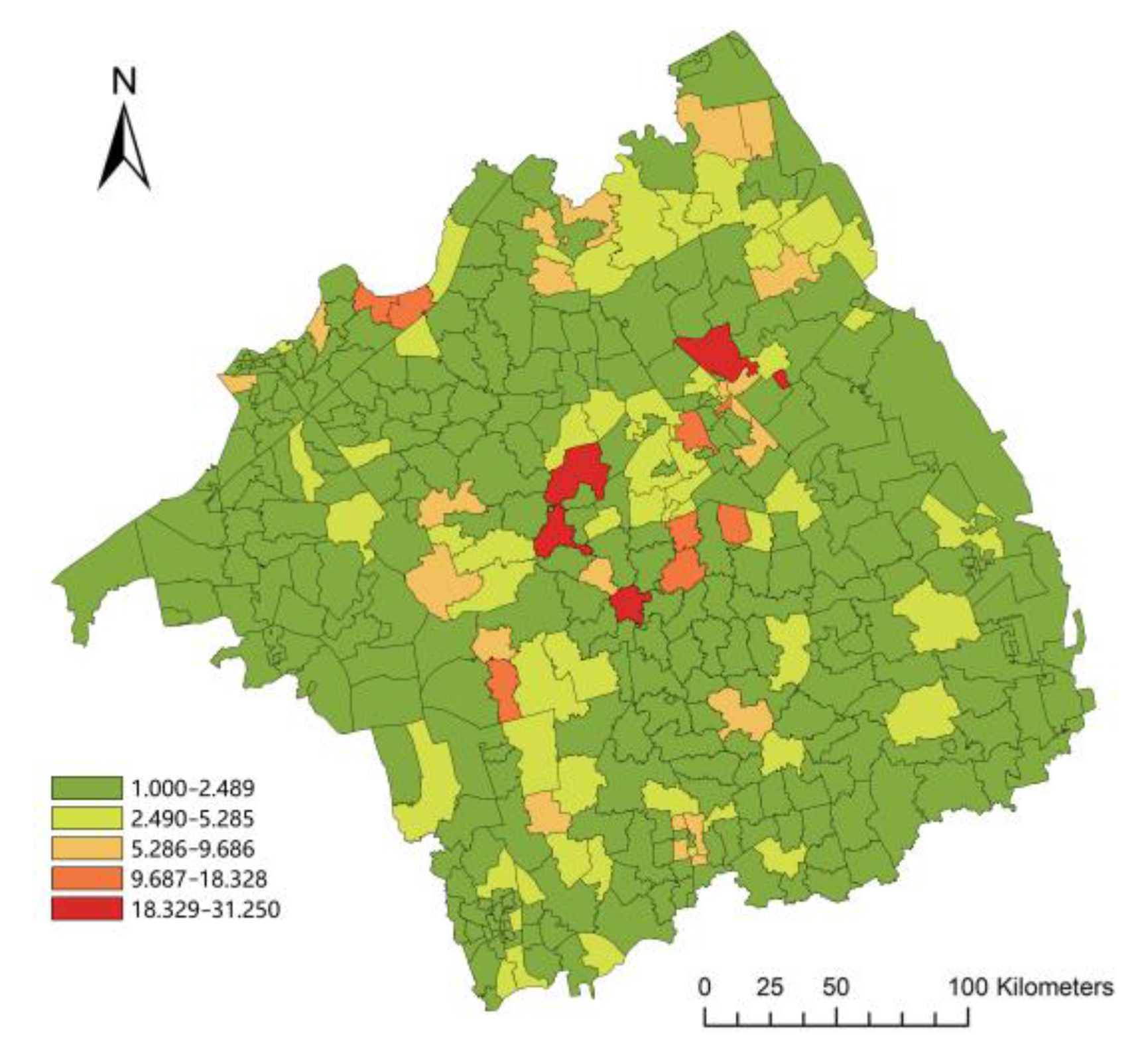
3.2.2. Spatial Association Analysis of Coupling Coordination

The relative length of the LISA time path can reveal the local spatial dependence and the stability of spatial structure from the perspective of time–space. The spatial characteristics of the coupling degree LISA time path relative length and the coupling coordination degree LISA time path relative length of the Lixiahe Plain composite ecosystem are similar through calculation. Among them, the township units with a long relative length of the LISA time path are mainly distributed in the northern and southwest areas, as well as land and water transportation ports and other important nodes and along the lines, such as Gaoyou, Baoying, Jiangdu, and other counties. The township units with a short relative length of the LISA time path are widely distributed, mainly in the central urban areas of mature municipal districts in the east, northwest, and south, or in general towns with a relatively weak foundation. This shows that from 2000 to 2020, the spatial structure of the coupling degree and the coupling coordination degree of remote towns and villages affected by geographical location and resource endowment, or the streets in the central urban areas affected by rapid urban development, etc., have little change (Figure 17 and Figure 18).

The LISA time path curvature of the coupling degree and coupling coordination degree in Lixiahe Plain is divided into five levels. The larger the curvature value is, the greater the influence of the spatial vitality value of the space itself is by the spatial vitality value of the neighborhood (overflow/polarization), and the township units have a more dynamic local spatial dependence direction and a more fluctuating growth process. On the whole, the time path curvature of the coupling degree and coupling coordination degree of the complex ecosystem in each township unit in Lixiahe Plain is greater than 1, and the curvature shows a decreasing trend from the regional center to the surrounding, indicating that the region has a strong spatial dependence, the local spatial structure of the central region is more dynamic, and the local spatial structure of the surrounding region is more stable.

In all 359 township units, the average value of LISA time path curvature of the coupling degree is 3.013, and the standard deviation is 3.731. The LISA time path curvature of 90 township units exceeds the average level of Lixiahe Plain. There are six township units with curvature greater than 16.164, which are distributed in Tinghu, Yandu, Xinghua, Gaoyou, and other county units. The average value of the LISA time path curvature of the coupling degree is 2.705, and the standard deviation is 3.547. The LISA time path curvature of 62 township units exceeds the average level of Lixiahe Plain. There are four township units with curvature greater than 18.329, which are distributed in Tinghu, Yandu, Xinghua, Gaoyou, and other county units (Figure 19 and Figure 20).

The LISA space–time transitions can identify the mutual transfer process characteristics of the local spatial association types of the coupling degree and coupling coordination degree. According to the calculation results of Moran’s I transfer probability of the local space of township units in Lixiahe Plain from 2000 to 2020, the local spatial association pattern of each township unit is not stable, and the spatial stability St of the coupling degree Moran’s I is 0.536, which indicates that the probability of the local spatial association of each township unit in Lixiahe Plain not experiencing a space–time transition in the past 20 years is 53.573%, and the probability of occurrence of a space–time transition is 46.427%. The spatial stability St of the coupling coordination degree Moran’s I is 0.519, and there are 3471 township units with space–time transitions, accounting for 48.075% of the total. Although there is certain transfer inertia in township units, there is still a great possibility of change.

From the perspective of space–time transition probability, the probability of space–time transition types of coupling degree are ranked from high to low: Type II (0.195) > Type I (0.165) > Type III (0.104). The highest transfer probability is type II, which is relatively stable in its own space–time transition, while the space–time transition in the neighborhood is more active. The second transfer probability is type I, which is more active in its own space–time transition, while the space–time transition in the neighborhood is more relatively stable. The lowest transfer probability is type III, and the space–time transition of itself and the neighborhood is relatively stable.

From the time traversal, when the coupling degree LISA space–time transition reaches a stable state, 47.2% of the township units remain in LL form, 22.0% in HH form, and 15.4% and 15.4% in LH and HL form, respectively. When the coupling coordination degree LISA space–time transition reaches a stable state, 47.8% of the township units remain in LL form, 21.2% in HH form, and 17.9% and 13.1% in LH and HL form, respectively. On the whole, the coupling degree and coupling coordination degree between the subsystems of township units in Lixiahe Plain is continuously strengthened. However, under the negative spatial spillover effect, many township units are still difficult to change their own limitation of focusing too much on the development of a single subsystem (

Table 8. Moran’s I transition probability matrix and spatial-temporal vicissitudes of the coupling degree of spatial vitality.

T/T + 1	HH (Plateau Type)	LH (Valley Type)	LL (Plain Type)	HL (Peak Type)	Type	n	Proportion	St
HH (Plateau type)	Type Ⅳ (0.080)	Type Ⅰ (0.011)	Type III (0.038)	Type II (0.038)	I	1190	0.165	0.536
LH (Valley type)	Type Ⅰ (0.041)	Type Ⅳ (0.069)	Type II (0.041)	Type III (0.009)	II	1408	0.195
LL (Plain type)	Type III (0.047)	Type II (0.063)	Type Ⅳ (0.324)	Type Ⅰ (0.044)	III	754	0.104
HL (Peak type)	Type II (0.052)	Type III (0.011)	Type Ⅰ (0.069)	Type Ⅳ (0.063)	Ⅳ	3868	0.536
Ergodic (Time traversal)	0.220	0.154	0.472	0.154	Sum	7220	1.000

and

Table 9. Moran’s I transition probability matrix and spatial-temporal vicissitudes of the coupling coordination degree of spatial vitality.

T/T + 1	HH (Plateau Type)	LH (Valley Type)	LL (Plain Type)	HL (Peak Type)	Type	n	Proportion	St
HH (Plateau type)	Type Ⅳ (0.074)	Type Ⅰ (0.011)	Type III (0.036)	Type II (0.038)	I	1170	0.162	0.519
LH (Valley type)	Type Ⅰ (0.036)	Type Ⅳ (0.069)	Type II (0.044)	Type III (0.000)	II	1646	0.228
LL (Plain type)	Type III (0.047)	Type II (0.091)	Type Ⅳ (0.321)	Type Ⅰ (0.038)	III	655	0.091
HL (Peak type)	Type II (0.055)	Type III (0.008)	Type Ⅰ (0.077)	Type Ⅳ (0.055)	Ⅳ	3749	0.519
Ergodic (Time traversal)	0.212	0.179	0.478	0.131	Sum	7220	1.000

).

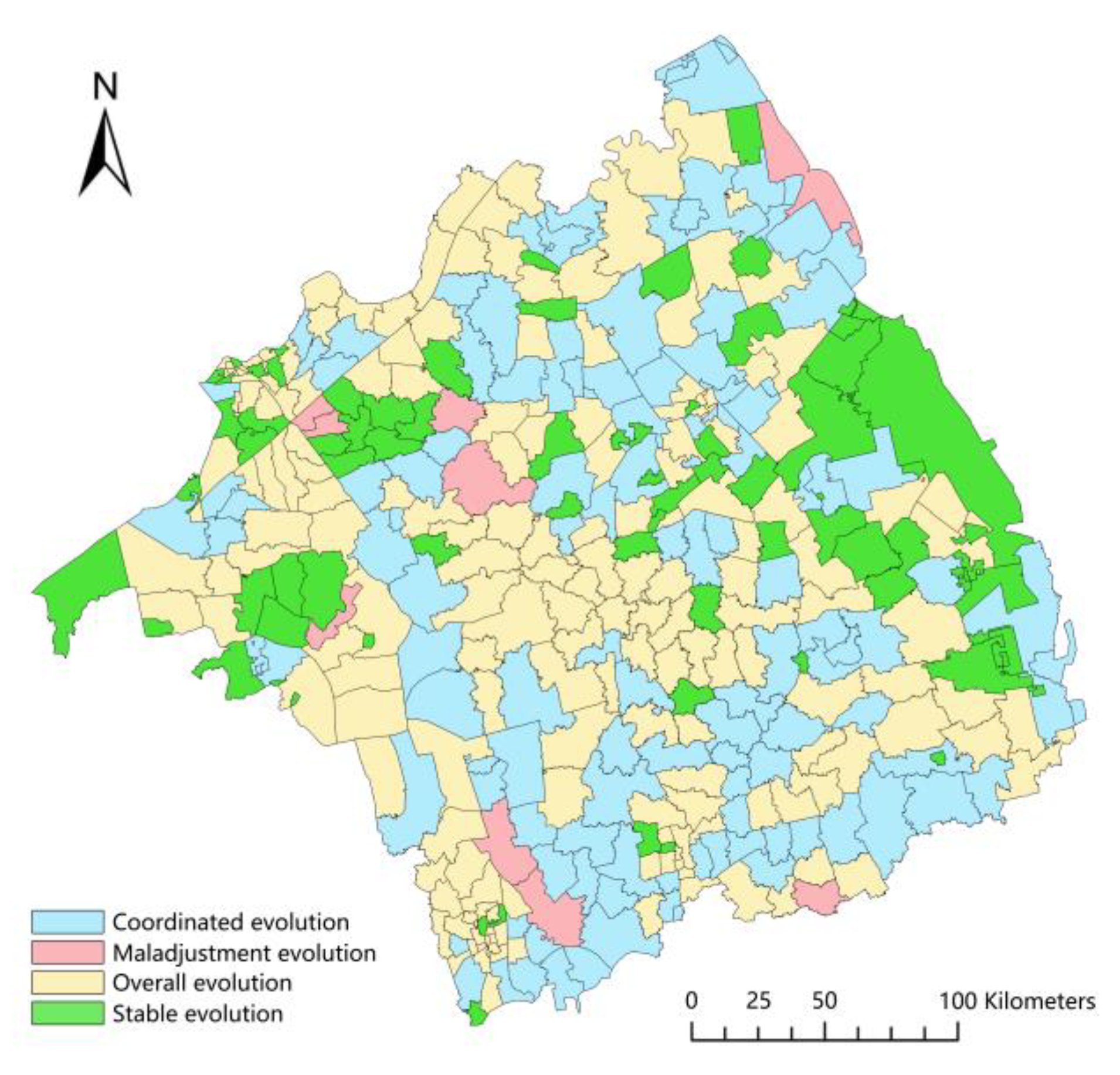
3.2.3. Evolution Type of Coupling Coordination

According to the spatio-temporal evolution trend of the coupling coordination of the spatial vitality of the complex ecosystem, the coupling and coordination evolution types of 359 township units in 20 counties units of Lixiahe Plain are divided into 4 types (Figure 21):

(1)

There are 107 township units of the coordinated evolution type, with small areas scattered throughout the whole Lixiahe Plain and large areas concentrated in the northeast and southern regions. From 2000 to 2020, the complex ecological subsystems promote each other, and both coupling coordination degree and spatial vitality value show an increasing trend. Among them, the average spatial vitality of this type in 2020 is 0.749, which is the best among the 4 types, the spatial vitality of the natural subsystem increases the fastest, and the economic subsystem increases the slowest.

(2)

There are nine township units of the maladjustment evolution type, the least in number, which are mainly distributed in the Yangzhou section of the Beijing-Hangzhou Canal in the southwest, the Huaihe River Channel and Sheyang Lake in the northwest, and the coastal area in the northeast. From 2000 to 2020, the complex ecological subsystems restrict each other, and both the coupling coordination degree and spatial vitality value showed a downward trend. Among them, the average spatial vitality of this type in 2020 is 0.627, which is second only to the coordinated evolution type, the spatial vitality of the social subsystem decreases the fastest, and the natural subsystem decreases the slowest.

(3)

There are 176 township units of the overall invariant type, the largest in number, with small areas scattered throughout the whole Lixiahe Plain and large areas concentrated in the northwest and central regions. The increase and decrease of the spatial vitality coordination indices of the complex ecosystem in this type of township unit are always within the range of ±0.1~1%. Among them, the average spatial vitality of this type in 2020 is 0.626, showing a similar coupling coordination type to that in 2000.

(4)

There are 69 township units of the stable invariant type, with small areas scattered throughout the middle of Lixiahe Plain and large areas concentrated in the eastern coastal and northwest lake areas. The increase and decrease of the spatial vitality coordination indices of the complex ecosystem in this type of township unit are always within the range of ±0~0.1%. Among them, the average spatial vitality of this type in 2020 is 0.508, which is the most stable and the worst among the four types, and the spatial vitality value also shows a slow downward trend.

4. Discussion and Conclusion

4.1. Discussion

Early studies on spatial vitality cannot be separated from the development of spatial structure theories such as city, street, and public space. From the beginning of the 20th century to the 1950s, most cities were still in the period of expansion and development. Optimizing urban space form through urban and rural planning and architectural design has become the main strategy to enhance the vitality and quality of cities, streets, and public spaces. Among them, the Compact City Theory advocates curbing urban sprawl, protecting suburban open spaces, reducing energy consumption, and creating diverse and vibrant urban life for people [65,66,67,68]. The Decentralized City Theory holds that the urban public transport system can enhance the spatial vitality of the surrounding countryside by closely connecting the central city with the surrounding communities [69,70,71,72]. After the middle of the 20th century, with the popularization of cars and the large-scale gathering of the urban population, people turned their attention to the outward relief of living and production functions such as urban residential areas and factories, and the optimization and adjustment of inner urban residential areas and transportation functions [73,74,75,76]. Since the 1960s, due to the popularization of new technologies and materials, the improvement of urban space vitality also pays more attention to the development of differentiation. People pay more and more attention to the external conditions of culture, history, society, and nature through the construction of space places [77]. Since the 1970s, with the demand for transformation and development of resource-based cities and the rise of the concept of ecological environment protection, people have incorporated ecological and environmental indices into the evaluation system of urban spatial quality and vitality construction, and the research on the urban spatial structure of the integration of nature, space, and human beings has gradually strengthened [78,79,80,81,82,83].

With the development of the times, the academic community’s attention to issues related to urban spatial vitality has continued to grow, and the number of research results has also been increasing. From the earliest attention to urban spatial structure and its theory to the research on spatial vitality indices and evaluation systems. Among them, the space vitality indices can be summarized into five aspects: space accessibility, functional diversity and mixing, environmental suitability and attractiveness, number and density of people, space scale, and shape [84,85,86,87,88]. The selection of evaluation indices elements has also undergone a transformation from traditional data types such as statistical yearbooks, questionnaire interviews, and field surveys to the application of spatio-temporal big data such as Internet technology and mobile communication technology [89]. Traditional methods such as the analytic hierarchy process, principal component analysis, semantic analysis, grey relational degree, and fuzzy comprehensive evaluation are still used to measure the evaluation index elements [90,91,92,93]. However, traditional data type acquisition methods, such as field research, have major defects in terms of research timeliness and research scale, which makes it impossible to conduct immediate and efficient analysis and measurement on a large number of large-scale regions. In addition, the questionnaire method is also subjective, and there is doubt about whether the results are universal and scientific. The use of new data types brought about by a single new technology, although to some extent, makes up for the shortcomings of traditional research, where research is generally suitable for specific research scenarios and special users.

The application and development of multi-source data fusion technology provide new ideas for solving the above problems. Since 2010, especially in the past five years, mobile signaling data, social network data, vehicle GPS data and intelligent traffic card swipe data, LBS heat map data, and POI data have been gradually widely used in the optimization of urban and rural spatial structure, as well as the research on the improvement of spatial vitality and spatial quality. In particular, the spatial pattern and spatio-temporal evolution characteristics of the spatial vitality value were measured and evaluated from the perspective of economic, social, and natural complex ecosystems. Under the background of the emergence of shrinking cities, the widening of inter-regional development differences, and the acute problem of urban-rural dual opposition, it provides a new idea for the study of the new sustainable development path of urban and rural areas [94,95,96,97].

4.2. Conclusions

4.2.1. Development Strategy of Township Units

The rapid development of the coordinated and evolved township unit economy, the continuous improvement of public service facilities and resource environment year by year, and the sufficient talent reserve are the growth poles for the improvement of regional comprehensive strength. On the one hand, it is necessary to accelerate the construction and optimization of the coordinated sustainable development mechanism among the subsystems of the township unit in Lixiahe Plain. On the other hand, it is also necessary to propose optimization measures for the industrial structure and planning layout of the economic subsystem elements to improve the current situation that the spatial vitality of the existing economic subsystem is weak, so as to maintain the ability of sustainable development in the region for a period of time in the future.

Although the number of township units with the maladjustment evolution type is the least, the coupling coordination index is second only to the coordinated evolution type, which has a good resource and environmental foundation, and superior transportation and location conditions. On the one hand, this type of township unit urgently needs to increase the construction of infrastructure and public service facilities such as transportation, education, medical care, sports, etc., to improve the quality of the living environment of each township unit. On the other hand, on the basis of optimizing the elements of each subsystem, the interaction relationship and coupling mechanism among the elements of each subsystem are sorted out, so as to improve the quality of the labor force and create more jobs.

As the type with the largest proportion of township units in the region, the spatial coupling coordination index of the overall invariant type determines the overall spatial vitality level of the region to a large extent. This type of township unit has always maintained a certain development potential in the past period of time, but the advantages of each subsystem element are not obvious. Therefore, transforming regional superior resources into productive forces is an important development strategy that needs to be urgently solved. On the one hand, it is necessary to enhance the vitality level of this type of space, and on the other hand, it is urgent to tap the potential of this type of space to develop in coordination and competition with other areas.

As one of the four types of township units with the most stable development and the worst performance, the biggest problem it faces is the lack of development impetus, unable to provide continuous vitality such as population and economy for subsequent development, and the loss of sustainable development ability. Therefore, this type of space needs to find or create new growth points for regional development. For example, by virtue of the resource advantages of the surrounding township units, it can provide them with supporting services such as education, medical care, human resources, and products, and enhance the matching degree and demand degree among the elements of the township subsystems in the region.

4.2.2. Innovation and Limitation of Research

The research takes night-time light data as the “measuring ruler” of the spatial vitality of the complex ecosystem, and takes POI data, land use remote sensing monitoring data, etc., as evaluation indices. On the one hand, the extraction method and measurement method of the spatial vitality factors of the complex ecosystem based on multi-source data were proposed. On the other hand, the spatio-temporal evolution track and spatial correlation characteristics of the coupling coordination between the spatial vitality of the township units in Lixiahe Plain were analyzed, and the evolution types of different township units were summarized, revealing the coupling mechanism of vitality space.

However, based on the extraction and analysis methods of multi-source data, such as night-time light, POI, and land use remote sensing monitoring, the efficiency of data processing and analysis on the macro- and meso-scale has been significantly improved compared with the traditional field survey and statistical data retrieval methods, and the consumption of manpower and material resources has been reduced. However, the above multi-source data also have their own shortcomings. For example, the accuracy of night light image data depends on the choice of data type and the advantages and disadvantages of data calibration methods. The earlier the POI data is, the smaller the data volume is, and the more data are missing, which makes this method unable to study from a longer time dimension.

References

1. Niu, W.Y. Understanding the Connotation of the Theory of Sustainable Development Commemorating the 20th Anniversary of the United Nations Rio Conference on Environment and Development. China’s Popul. Resour. Environ. 2012, 22, 9–14. [Google Scholar] [CrossRef]
2. Bai, X.M.; Shi, P.J.; Liu, Y.S. Realizing China’s urban dream. Nature 2014, 509, 158–160. [Google Scholar] [CrossRef] [PubMed] [Green Version]
3. Xue, B.; Li, H.Q.; Huang, B.J.; Wang, H.M.; Zhao, X.Y.; Fang, K.; Chen, C.; Chen, W.Q.; Shi, L.; Gou, X.H. Data driven research on social economic natural complex ecosystem: Scale, process and its decision-making correlation. J. Appl. Ecol. 2022, 33, 3169–3176. [Google Scholar] [CrossRef]
4. Fang, C.L.; Zhou, C.H.; Gu, C.L.; Chen, L.D.; Li, S.C. The theoretical framework and technical path for the analysis of the interactive coupling effect between urbanization and ecological environment in mega urban agglomeration areas. Acta Geogr. Sin. 2016, 71, 531–550. [Google Scholar] [CrossRef]
5. De Knegt, H.J.; van Langevelde, F.; Coughenour, M.B.; Skidmore, A.K.; de Boer, W.F.; Heitkönig, I.M.A.; Knox, N.M.; Slotow, R.; van der Waal, C.; Prins, H.H.T. Spatial autocorrelation and the scaling of species-environment relationships. Ecology 2010, 91, 2455–2465. [Google Scholar] [CrossRef] [Green Version]
6. Batty, M. The Size, Scale, and Shape of Cities. Science 2008, 319, 769–771. [Google Scholar] [CrossRef] [PubMed] [Green Version]
7. Gong, Y.X.; Ji, X.; Hong, X.C.; Cheng, S.S. Correlation Analysis of Landscape Structure and Water Quality in Suzhou National Wetland Park, China. Water 2021, 13, 2075. [Google Scholar] [CrossRef]
8. Costanza, R. Ecosystem health and ecological engineering. Ecol. Eng. 2012, 45, 24–29. [Google Scholar] [CrossRef] [Green Version]
9. Li, J.C.; Shi, L.M.; Xu, A.T. Discussion on the evaluation index system of high-quality development. Stat. Res. 2019, 36, 4–14. [Google Scholar] [CrossRef]
10. Roberts, M.G.; Yang, G.A. International progress in research methods of sustainable development comparison between vulnerability analysis methods and sustainable livelihood methods. Prog. Geogr. Sci. 2003, 1, 11–21. [Google Scholar] [CrossRef]
11. Bakshi, B. A themodynamic framework for ecologically conscious process system engineer. Comput. Chem. Eng. 2002, 26, 269–282. [Google Scholar] [CrossRef]
12. Wang, Z.Y.; Ma, J.J.; Chen, X.X.; Zhao, D.; Teng, T.; Yang, Y.C. Ecological health assessment of three core development areas in Xi’an based on emergy analysis. Soil Water Conserv. Res. 2018, 25, 317–323. [Google Scholar] [CrossRef]
13. Khanam, S.; Siddiqui, J.; Talib, F. A DEMATEL approach for prioritizing the TQM enablers and IT resources in the Indian ICT industry. Soc. Sci. Electron. Publ. 2016, 3, 11–29. [Google Scholar] [CrossRef] [Green Version]
14. Tscharner, R.V. Place Makers: Creating Public Art That Tells You Where You Are: With an Essay on Planning and Policy; Houghton Mifflin Harcourt: Boston, MA, USA, 1987. [Google Scholar]
15. Schneekloth, L.H.; Shibley, R.G. The Art and Practice of Building Communities; Wiley: Hoboken, NJ, USA, 1995. [Google Scholar]
16. Trancik, R. Finding Lost Space: Theories of Urban Design; John Wiley & Sons: New York, NY, USA, 1986. [Google Scholar]
17. Montgomery, J. Making a city: Urbanity, vitality and urban design. J. Urban Des. 1998, 3, 93–116. [Google Scholar] [CrossRef]
18. Biddulph, M. Street design and street use: Comparing traffic calmed and home zone streets. J. Urban Des. 2012, 17, 213–232. [Google Scholar] [CrossRef]
19. Ewing, R.; Handy, S. Measuring the unmeasurable: Urban design qualities related to walkability. J. Urban Des. 2009, 14, 65–84. [Google Scholar] [CrossRef]
20. Wang, H.; Jiang, D. Evaluation system research on vitality of urban public space. J. Railw. Sci. Eng. 2012, 9, 56–60. [Google Scholar] [CrossRef]
21. Chen, F.; Lin, J.; Zhu, X. Factor analysis on public space activity evaluation of winter cities. J. Harbin Inst. Technol. 2017, 49, 179–188. [Google Scholar] [CrossRef]
22. Rundle, A.G.; Bader, M.D.M.; Richards, C.A.; Neckerman, K.M.; Teitler, J.O. Using Google Street View to Audit Neighborhood Environments. Am. J. Prev. Med. 2011, 40, 94–100. [Google Scholar] [CrossRef] [Green Version]
23. Naik, N.; Philipoom, J.; Raskar, R.; Hidalgo, C. Streetscore: Predicting the Perceived Safety of One Million Streetscapes. In Proceedings of the IEEE Conference on Computer Vision and Pattern Recognition Workshops (CVPRW), Columbus, OH, USA, 23–28 June 2014; pp. 793–799. Available online: https://ieeexplore.ieee.org/document/6910072 (accessed on 1 December 2022).
24. Sarkar, C.; Webster, C.; Pryor, M.; Tang, D.; Melbourne, S.; Zhang, X.H.; Liu, J.Z. Exploring Associations between Urban Green, Street Design and Walking: Results from the Greater London Boroughs. Landsc. Urban Plan. 2015, 143, 112–125. [Google Scholar] [CrossRef]
25. Luo, S.Z.X.; Zhen, F. How to evaluate public space vitality based on mobile phone data: An empirical analysis of Nanjing’s parks. Geogr. Res. 2019, 38, 1594–1608. Available online: http://www.dlyj.ac.cn/CN/10.11821/dlyj020180756 (accessed on 1 December 2022).
26. Dahal, R.P.; Grala, R.K.; Gordon, J.S.; Munn, D.R.; Cummings, J.R. A hedonic pricing method to estimate the value of waterfronts in the Gulf of Mexico. Urban For. Urban Green. 2019, 41, 185–194. [Google Scholar] [CrossRef]
27. Liu, S.Y.; Zhao, P.J.; Liang, J.S. Study on Urban Vitality Based on LBS Data: A Case of Beijing within 6th Ring Road. Areal Res. Dev. 2018, 37, 64–69,87. Available online: http://hdl.handle.net/20.500.11897/572803 (accessed on 1 December 2022).
28. Wang, W.Q.; Ma, X.J. Vitality Assessment of Waterfront Public Space Based on Multi-Source Data: A Case Study of the Huangpu River Waterfront. Urban Plan. Forum 2020, 1, 48–56. [Google Scholar] [CrossRef]
29. Yang, X.; Fang, Z.; Xu, Y.; Shaw, S.-L.; Zhao, Z.; Yin, L.; Zhang, Z.; Lin, Y. Understanding Spatiotemporal Patterns of Human Convergence and Divergence Using Mobile Phone Location Data. ISPRS Int. J. Geo-Inf. 2016, 5, 177. [Google Scholar] [CrossRef] [Green Version]
30. Zeng, C.; Song, Y.; He, Q.Q.; Shen, F.X. Spatially Explicit Assessment on Urban Vitality: Case Studies in Chicago and Wuhan. Sustain. Cities Soc. 2018, 40, 296–306. [Google Scholar] [CrossRef]
31. Liu, S.; Lai, S. Measurement of Urban Public Space Vitality Based on Big Data. Landsc. Archit. 2019, 26, 24–28. [Google Scholar] [CrossRef]
32. Lei, Y.; Lu, C.; Su, Y.; Huang, Y. Research on the coupling relationship between urban vitality and urban sprawl based on the multi-source night-time light data—A case study of the west Taiwan strait urban agglomeration. Hum. Geogr. 2022, 37, 119–131. [Google Scholar] [CrossRef]
33. Wang, M.; Chen, M.X.; Song, H.Y. Influence of Coupled Coordination of Habitat Quality and Recreation Services on the Vitality of Waterfront Space. J. Chin. Urban For. 2022, 20, 7–13. [Google Scholar] [CrossRef]
34. Zhang, Y.; Ji, X.; Sun, L.; Gong, Y.X. Spatial Evaluation of Villages and Towns Based on Multi-Source Data and Digital Technology: A Case Study of Suining County of Northern Jiangsu. Sustainability 2022, 14, 7603. [Google Scholar] [CrossRef]
35. Ye, J.; Yang, X.H.; Jiang, D. The grid scale effect analysis on town leveled population statistical data spatialization. J. Geo-Inf. Sci. 2010, 12, 40–47. Available online: http://www.dqxxkx.cn/CN/Y2010/V12/I1/40 (accessed on 1 December 2022).
36. Shi, K.F.; Yu, B.L.; Huang, Y.X.; Hu, Y.J.; Yin, B.; Chen, Z.Q.; Chen, L.J.; Wu, J.P. Evaluating the ability of NPP-VIIRS nighttime light data to estimate the gross domestic product and the electric power consumption of China at multiple scales: A comparison with DMSP-OLS data. Remote Sens. 2014, 6, 1705–1724. [Google Scholar] [CrossRef] [Green Version]
37. Turner, B.L.; Skole, D.L.; Sanderson, S.; Fischer, G.; Fresco, L.; Leemans, R. Land Use and Land Cover Change. Science/Research Plan; IGBP Report No. 35 & HDP report No. 7; IGBP: Stockholm, Sweden, 1995. [Google Scholar] [CrossRef]
38. Wang, D.; Ji, X.; Li, C.; Gong, Y.X. Spatiotemporal Variations of Landscape Ecological Risks in a Resource-Based City under Transformation. Sustainability 2021, 13, 5297. [Google Scholar] [CrossRef]
39. Diao, M.; Zhu, Y.; Ferreira, J.; Ratti, C. Inferring Individual Daily Activities from Mobile Phone Traces: A Boston Example. Environ. Plan. B Plan. Des. 2016, 43, 920–940. [Google Scholar] [CrossRef] [Green Version]
40. Xu, Y.; Shaw, S.L.; Zhao, Z.L.; Yin, L.; Lu, F.; Chen, J.; Fang, Z.X.; Li, Q.Q. Another Tale of Two Cities: Understanding Human Activity Space Using Actively Tracked Cellphone Location Data. Ann. Am. Assoc. Geogr. 2016, 106, 489–502. Available online: https://www.tandfonline.com/doi/full/10.1080/00045608.2015.1120147 (accessed on 1 December 2022).
41. Wang, W.Q.; Ma, X.J. Research on the vitality evaluation of waterfront public space based on multi-source data taking the Huangpu River waterfront as an example. J. Urban Plan. 2020, 1, 48–56. [Google Scholar] [CrossRef]
42. Wu, K.M.; Zhang, H.O.; Wang, Y.; Wu, Q.T.; Ye, Y.Y. Identify of the multiple types of commercial center in Guangzhou and its spatial pattern. Prog. Geogr. 2016, 35, 963–974. [Google Scholar] [CrossRef] [Green Version]
43. Wang, J.F.; Ge, Y.; Li, L.F.; Meng, B.; Wu, J.L.; Bo, Y.C.; Du, S.H.; Liao, Y.L.; Hu, M.G.; Xu, C.D. Spatiotemporal data analysis in geography. Acta Geogr. Sin. 2014, 69, 1326–1345. [Google Scholar] [CrossRef]
44. Jiang, S.; Alves, A.; Rodrigues, F.; Ferreira, J.; Pereira, F.C. Mining point of interest data from social networks for urban land use classification and disaggregation. Comput. Environ. Urban Syst. 2015, 53, 36–46. [Google Scholar] [CrossRef] [Green Version]
45. Chen, Y.M.; Liu, X.P.; Li, X. Analyzing parcel-level relationships between urban land expansion and activity changes by integrating landsat and nighttime light data. Remote Sens. 2017, 9, 164. [Google Scholar] [CrossRef] [Green Version]
46. Dang, L.J.; Xu, Y.; Gao, Y. Assessment method of functional land use classification and spatial system: A case study of Yangou Watershed. Res. Soil Water Conserv. 2014, 21, 193–197. [Google Scholar] [CrossRef]
47. Long, H.L.; Liu, Y.Q.; Li, T.T.; Wang, J.; Liu, A.X. A primary study on ecological land use classification. Ecol. Environ. Sci. 2015, 24, 1–7. [Google Scholar] [CrossRef]
48. Elvidge, C.D.; Baugh, K.E.; Zhizhin, M.; Hsu, F.C. Why VIIRS data are superior to DMSP for mapping nighttime lights. Proc. Asia Pac. Adv. Netw. 2013, 35, 62–69. [Google Scholar] [CrossRef]
49. Li, X.; Xu, H.M.; Chen, X.L.; Li, C. Potential of NPP-VIIRS nighttime light imagery for modeling the regional economy of China. Remote Sens. 2013, 5, 3057–3081. [Google Scholar] [CrossRef] [Green Version]
50. Elvidge, C.D.; Ziskin, D.; Baugh, K.E.; Tuttle, B.T.; Ghosh, T.; Pack, D.W.; Erwin, E.H.; Zhizhin, M. A fifteen year record of global natural gas flaring derived from satellite data. Energies 2009, 2, 595–622. [Google Scholar] [CrossRef]
51. Wu, J.S.; He, S.B.; Peng, J.; Li, W.F.; Zhong, X.H. Intercalibration of DMSP/OLS night-time light data by the invariant region method. Int. J. Remote Sens. 2013, 34, 7356–7368. [Google Scholar] [CrossRef]
52. Zhuo, L.; Zheng, J.; Zhang, X.F.; Li, J.; Liu, L. An improved method of night-time light saturation reduction based on EVI. Int. J. Remote Sens. 2015, 36, 4114–4130. [Google Scholar] [CrossRef]
53. Yu, B.L.; Tang, M.; Wu, Q.S.; Yang, C.S.; Deng, S.Q.; Shi, K.F.; Peng, C.; Wu, J.P.; Chen, Z.Q. Urban Built-Up Area Extraction from Log-Transformed NPP-VIIRS Nighttime Light Composite Data. IEEE Geosci. Remote Sens. Lett. 2018, 15, 1279–1283. [Google Scholar] [CrossRef]
54. Li, X.; Li, D.R.; Xu, H.M.; Wu, C.Q. Intercalibration between DMSP/OLS and VIIRS night-time light images to evaluate city light dynamics of Syria’s major human settlement during Syrian Civil War. Int. J. Remote Sens. 2017, 38, 5934–5951. [Google Scholar] [CrossRef]
55. Li, M.; Shen, Z.; Hao, X. Revealing the relationship between spatio-temporal distribution of population and urban function with social media data. GeoJournal 2016, 81, 919–935. Available online: https://www.jstor.org/stable/44132611 (accessed on 1 December 2022).
56. Zeng, C.Q.; Zhou, Y.; Wang, S.X.; Yan, F.L.; Zhao, Q. Population spatialization in China based on night-time imagery and land use data. Int. J. Remote Sens. 2011, 32, 9599–9620. [Google Scholar] [CrossRef]
57. Wei, Y.; Liu, H.X.; Song, W.; Yu, B.L.; Xiu, C.L. Normalization of time series DMSP-OLS nighttime light images for urban growth analysis with Pseudo Invariant Features. Landsc. Urban Plan. 2014, 128, 1–13. [Google Scholar] [CrossRef]
58. Dong, P.L.; Ramesh, S.; Nepali, A. Evaluation of small-area population estimation using LiDAR, Landsat TM and parcel data. Int. J. Remote Sens. 2010, 31, 5571–5586. [Google Scholar] [CrossRef]
59. Alshehri, S.A.; Rezgui, Y.; Li, H. Disaster community resilience assessment method: A consensus-based Delphi and AHP approach. Nat. Hazards 2015, 78, 395–416. [Google Scholar] [CrossRef]
60. Wang, F.X.; Mao, A.H.; Li, H.L.; Jia, M.L. Quality measurement and spatial difference analysis of urbanization in Shandong Province based on entropy method. Geogr. Sci. 2013, 33, 1323–1329. [Google Scholar] [CrossRef]
61. Niu, X.; Du, Z.; Li, T. Evaluation of regional urbanization level based on a new urbanization perspective—Taking 10 cities under the jurisdiction of Shaanxi Province as an example. Arid Zone Geogr. 2013, 36, 354–363. [Google Scholar] [CrossRef]
62. Kline, J.D.; Moses, A.; Alig, R.J. Integrating Urbanization into Landscape-level Ecological Assessments. Ecosystems. 2001, 4, 3–18. [Google Scholar] [CrossRef]
63. Kim, D.S.; Mizuno, K.; Kobayashi, S. Analysis of urbanization characteristics causing farmland loss in a rapid growth area using GIS and RS. Paddy Water Environ. 2003, 1, 189–199. [Google Scholar] [CrossRef]
64. Zhu, Q.; Fu, X. The Review of Visual Analysis Methods of Multi-modal Spatio-temporal Big Data. Acta Geogr. Sin. 2017, 46, 1672–1677. [Google Scholar] [CrossRef]
65. Jin, Q.; Wang, Y. Le Corbusier. Radiant City; China Architecture & Building Press: Beijing, China, 2011. [Google Scholar]
66. Hoyt, H. One Hundred Years of Land Values in Chicago; Jia, Z., Ed.; Economic Science Press: Beijing, China, 2011. [Google Scholar]
67. Feng, C.C.; Yang, Z.W. Review of Urban Land Use in Europe and America. Urban Plan. Int. 1998, 19, 2–9. Available online: https://kns.cnki.net/kcms2/article/abstract?v=20d6x5-H6Wkv1G89iOUuveKoJGJsPSzMx78hQKW6q0ndrKF7MbPFkbvpXFk4DObatI3_z45bFiPbNs2MW9oKarlICCa77imOB4GeM0ykzc_FjJ3dxtV9Qw==&uniplatform=NZKPT&language=CHS (accessed on 1 December 2022).
68. Gu, K. Theory and Method of Urban Form—Explore a comprehensive and rational research framework. City Plan. Rev. 2001, 25, 36–42. Available online: https://kns.cnki.net/kcms2/article/abstract?v=20d6x5-H6WmrJry1JpLlRDPuInM5QnxMHrK5KBJivyotpLo9clWoQiYjtwSnXqq7AP4ZaeSdBYn9gI8VHw7pWFkJazPTubD22zZs3kbHIoe8W5gjeMtJZQ==&uniplatform=NZKPT&language=CHS (accessed on 1 December 2022).
69. Eliel, S. City: Its Growth, Its Decay, Its Future; Gu, Q., Ed.; China Architecture & Building Press: Beijing, China, 1986. [Google Scholar]
70. Ebenezer, H. Garden Cities of Tomorrow; The Commercial Press: Beijing, China, 2010. [Google Scholar]
71. Shi, Y.S. A Summary of Village and Town Systems Research at Home and Abroad. Urban Plan. Int. 2007, 4, 84–88. Available online: https://kns.cnki.net/kcms/detail/detail.aspx?dbcode=CJFD&dbname=CJFD2007&filename=GWCG200704017&uniplatform=NZKPT&v=2ycJ-7IoWDI3MvwcGUer-IVKjYYucdcXd869SloDcKW45zmBgEwk-RVneiVK7pyP (accessed on 1 December 2022).
72. He, S.W. The original sin of urban sprawl—On the History of Decentralism. Planners 2008, 15, 97–100. Available online: https://kns.cnki.net/kcms2/article/abstract?v=20d6x5-H6WnjFd-nWuZ_Ov9ROH2sSoWXSD5dvWI04RSlZUPPYA6E9LMnj8uKc1G8hpolMmN4Sf84MusfltkpOfTjJmjgRISX3fQ4TM8SDVQcHiLAuHujJw==&uniplatform=NZKPT (accessed on 1 December 2022).
73. Liang, J. A reexamination of the market principle in central place theory. Acta Geogr. Sin. 2022, 77, 1892–1906. Available online: https://kns.cnki.net/kcms2/article/abstract?v=20d6x5-H6Wk2gWsXojirPAY7EoiXQlg-54YkQEi3V5j3Tm53NqyFwOTfeva3ftO0UH4S84IRNvCbpP_k6zUAcZT0NQI0vtmr1De6uYzjhhNk3hBH1RNewRqCVIQlSE3y&uniplatform=NZKPT&language=CHS (accessed on 1 December 2022).
74. Liang, J.S. Central place system substitutability and point-axle system. Acta Geogr. Sin. 1998, S1, 204–211. Available online: https://kns.cnki.net/kcms/detail/detail.aspx?dbcode=CJFD&dbname=CJFD9899&filename=DLXB1998S1025&uniplatform=NZKPT&v=97EOHO6OO6EFCBWx_4qcXYQwHlqs1IIu5FA2Gqd6nTtIT0L2WAw4m_Eq6qEc6yeo (accessed on 1 December 2022).
75. Li, D.Q.; Zheng, G.; Luo, X. Revisiting neighborhood unit and residential community: A knowledge transfer perspective. City Plan. Rev. 2021, 45, 36–42. Available online: https://kns.cnki.net/kcms/detail/detail.aspx?dbcode=CJFD&dbname=CJFDLAST2021&filename=CSGH202111008&uniplatform=NZKPT&v=e0VWQrSXHmS-j_2AFmW-d7reep9NJnUVTaBQ4Xp2InbpGUmvcLDpcl6S6xTL6AGW (accessed on 1 December 2022).
76. Qiu, B.X. Six transitions in the evolution of western urban planning theories since the 19th century. Planners 2003, 10, 5–10. Available online: https://kns.cnki.net/kcms2/article/abstract?v=20d6x5-H6Wl3dDB_cA_YvlSUPnMbCZM-BXoPtMvzcg888XyIlpdlnxzkHGGKqRPKnc_77hfmHAifmbOG0TcF9ZRvS0F_TmwDFBbV0UTqH9_cRMHPTciImQ==&uniplatform=NZKPT&language=CHS (accessed on 1 December 2022).
77. Tiesdale, S.; Heath, T. Revitaliazing Historic Urban Quarters; Zhang, M., Dong, W., Eds.; China Architecture & Building Press: Beijing, China, 2006. [Google Scholar]
78. Huang, G.; Chen, Y. Study on the concept of eco city and its planning and design method. City Plan. Rev. 1997, 21, 17–20. Available online: https://kns.cnki.net/kcms2/article/abstract?v=20d6x5-H6WnBPoWI2Rzvtw5D1Tlx-oWXDWfHWDvhmgceeoKNAUXdY9Fv6kagdG7XOP5B2_zfN-qTOMvLhhDkCRpoivZE1IpOMlG4kgEQ-K1VgB4rNDz60A==&uniplatform=NZKPT (accessed on 1 December 2022).
79. Wu, L.Y. “Landscape City” and Urban Development in China in the 21st Century. Archit. J. 1993, 33, 4–8. Available online: https://kns.cnki.net/kcms2/article/abstract?v=20d6x5-H6WmX341YZY5qgNxi3B8aQ5gWsY-aIYa0wwJUP-6ZmlZdNVn9ngcnDkkflxE0g8FDrfu1j9w8hvds1AVJdcQ-akEo8zVpJfQ6nKhZCxhlPOlYvw==&uniplatform=NZKPT&language=CHS (accessed on 1 December 2022).
80. Liu, Y.; Li, R.; Song, X. Summary and Comment of the Correlation Study of Urbanization and Urban Eco-Environment. China Popul. Resour. Environ. 2005, 15, 55–60. Available online: https://kns.cnki.net/kcms2/article/abstract?v=20d6x5-H6WmgdEnnzjDezUQl6zMnE1823NmBoTVs6YBwujVYVcxTKjOFHWXDx7ucBOn39s_mpWuL8PKLC9Kx33VIO3XT_f5xnKe-W6Dj_KUIcloaXH4N7Q==&uniplatform=NZKPT&language=CHS (accessed on 1 December 2022).
81. Li, T. New Progress in Study on Resilient Cities. Urban Plan. Int. 2017, 32, 15–25. Available online: https://kns.cnki.net/kcms2/article/abstract?v=20d6x5-H6WlaXWn7MmdJxy9mFODYOAQpR7CpWRCo6aRlctyo7TpkKvsgORNpH8Ms9WteHYUs5Uk0hclJsftm9M-0iErAdT97R6tuR1C6QBUz71mJ-Hv7YCB7RAvRvoQZ&uniplatform=NZKPT&language=CHS (accessed on 1 December 2022). [CrossRef]
82. Liu, Z.L.; Dai, Y.X.; Dong, C.G.; Qi, Y. Low-Carbon City: Concepts, International Practice and Implications for China. Urban Dev. Study 2009, 16, 1–7,12. Available online: https://kns.cnki.net/kcms2/article/abstract?v=20d6x5-H6WlVHWXtGQOS0J9_9v6U81FDTk7ilW8Pa1tip0rjam08fajcdv2Z-_2_UFVmvPbWTuHmXUvzGzRB04l6OQ9YNTh_zEr4fTeDeCMOotjFFc4T8Q==&uniplatform=NZKPT&language=CHS (accessed on 1 December 2022).
83. Yu, K.J.; Li, D.H.; Yuan, H.; Fu, W.; Qiao, Q.; Wang, S.S. “Sponge City”: Theory and Practice. City Plan. Rev. 2015, 39, 26–36. Available online: https://kns.cnki.net/kcms2/article/abstract?v=20d6x5-H6Wm9XSxhgF84_FG7dFSbUNDncwAYeznCculkka0TruCsJzrqNh-MStfWW9oaTPrUcqxdH3qO0x_-frET-_AMVpASSjmYMbLZJqicjsSZJ7Fghbc6V9I7Abn8&uniplatform=NZKPT&language=CHS (accessed on 1 December 2022).
84. Jacobs, J. The Death and Life of Great American Cities; Vintage: New York, NY, USA, 1961. [Google Scholar]
85. Lynch, K. Good City Form; The MIT Press: Cambridge, MA, USA, 1984. [Google Scholar]
86. Gale, J. Humanized City; Xu, Z., Ed.; China Architecture & Building Press: Beijing, China, 2010. [Google Scholar]
87. Bentley, I. Resonance Design of Building Environment; Ji, X., Gao, Y., Eds.; Dalian University of Technology Press: Dalian, China, 2002. [Google Scholar]
88. Zou, Q.; Li, G. Public Space Construction of Urban Resettlement Community Based on Analysis of Vitality Characteristics: Taking the 6 Resettlement Communities of Suzhou as Examples. Sci. Geogr. Sin. 2018, 38, 747–754. [Google Scholar] [CrossRef]
89. Kendall, A.; Badrinarayanan, V.; Cipolla, R. Bayesian SegNet: Model Uncertainty in Deep Convolutional Encoder-Decoder Architectures for Scene Understanding. IEICE Trans. Fundam. Electron. Commun. Comput. Sci. 2015. [Google Scholar] [CrossRef]
90. Long, Y.; Zhou, Y. Quantitative Evaluation on Street Vibrancy and Its Impact Factors: A case Study of Chengdu. New Archit. 2016, 34, 52–57. Available online: https://kns.cnki.net/kcms2/article/abstract?v=20d6x5-H6Wn-xyz96dQBNf3h5OlDZ-GOK8lfBABeRYd48b1_1flyJ7MOfHFeLAA94vv-uY81Nt1S7qp6hdEWZRySID1JKrawF6MTKbV8Mp0lK6OxD0Sihj1y4TUyL3vs&uniplatform=NZKPT (accessed on 1 December 2022).
91. Long, Y.; Liu, L. Four Transformations of Chinese Quantitative Urban Research in the New Data Environment. Urban Plan. Int. 2017, 32, 64–73. Available online: https://kns.cnki.net/kcms2/article/abstract?v=20d6x5-H6WmqFWumc_ui2l6xRR89AiZkFBAeroBak7derVI0ywA0crJey7T7XoHZdVZV0C7WnAqvzWUNKQVuXoF7xpEOquoF0gEjZx8BQBayscVPRVAz0k_MXoc2PS-Q&uniplatform=NZKPT&language=CHS (accessed on 1 December 2022). [CrossRef] [Green Version]
92. Wang, Y.Z. Research on Urban Spatial Vitality Characteristic Evaluation and Internal Mechanism of Shanghai Central City Based on Mobile Phone Signaling Data; Southeast University: Dhaka, Bangladesh, 2017. [Google Scholar]
93. Qiu, Y. Research on Urban Street Spatial Vitality Evaluation Based on Multi-Source Data: A Case Study of Suzhou Ancient Downtown; Suzhou University of Science and Technology: Suzhou, China, 2019; Available online: https://kns.cnki.net/kcms/detail/detail.aspx?dbcode=CMFD&dbname=CMFD202001&filename=1019191965.nh&uniplatform=NZKPT&v=8rdYUdN8h3rs77EvMzl4Wbk-vxotFDQwij34hbNzcuB75o8o8zJCxQotob48WYLM (accessed on 1 December 2022).
94. Wakamiya, S.; Lee, R.; Sumiya, K. Urban Area Characterization Based on Semantics of Crowd Activities in Twitter. Pers. Ubiquitous Comput. 2011, 4, 108–123. Available online: https://dl.acm.org/doi/10.1007/s00779-012-0510-9 (accessed on 1 December 2022).
95. Mark, B.; Nick, M. Microscopic Simulations of Complex Metropolitan Dynamics; Complex City Workshop: Amsterdam, The Netherlands, 2011. [Google Scholar]
96. Steiger, E.; Westerholt, R.; Resch, B.; Zipf, A. Twitter as an indicator for whereabouts of people? Correlating Twitter with UK census data. Comput. Environ. Urban Syst. 2015, 54, 255–265. [Google Scholar] [CrossRef]
97. Malleson, N.; Birkin, M. Analysis of crime patterns through the integration of an agent-based model and a population microsimulation. Comput. Environ. Urban Syst. 2012, 36, 551–561. [Google Scholar] [CrossRef]
Figure 1. The location of the study area and the administrative division of counties and towns.
Sustainability 15 02141 g001
Figure 2. Correction process of night-time light data.
Sustainability 15 02141 g002
Figure 3. Space vitality type identification process for the complex ecosystem in Lixiahe Plain.
Sustainability 15 02141 g003
Figure 4. Spatial vitality score of the complex ecosystem.
Sustainability 15 02141 g004
Figure 5. Spatial vitality score of the economic subsystem.
Sustainability 15 02141 g005
Figure 6. Spatial vitality score of the social subsystem.
Sustainability 15 02141 g006
Figure 7. Spatial vitality score of the natural subsystem.
Sustainability 15 02141 g007
Figure 8. Spatial vitality score of the population subsystem.
Sustainability 15 02141 g008
Figure 9. Spatial vitality change curve of the complex ecosystem and subsystem.
Sustainability 15 02141 g009
Figure 10. Spatial vitality level distribution of the complex ecosystem at township units.
Sustainability 15 02141 g010
Figure 11. Spatial distribution of the spatial vitality level.
Sustainability 15 02141 g011
Figure 12. Spatial distribution of vigorous vitality.
Sustainability 15 02141 g012
Figure 13. Classification chart of the coupling degree of spatial vitality in 2000–2020.
Sustainability 15 02141 g013
Figure 14. Classification chart of the coupling coordination degree of spatial vitality in 2000–2020.
Sustainability 15 02141 g014
Figure 15. LISA cluster chart of the coupling degree of spatial vitality in Lixiahe region in 2000–2020.
Sustainability 15 02141 g015
Figure 16. LISA cluster chart of coupling coordination degree of spatial vitality in Lixiahe region in 2000–2020.
Sustainability 15 02141 g016
Figure 17. LISA time path length of the coupling degree of spatial vitality in Lixiahe region.
Sustainability 15 02141 g017
Figure 18. LISA time path length of the coupling coordination degree of spatial vitality in Lixiahe region.
Sustainability 15 02141 g018
Figure 19. LISA time path curvature of the coupling degree of spatial vitality in Lixiahe region.
Sustainability 15 02141 g019
Figure 20. LISA time path curvature of the coupling coordination degree of spatial vitality in Lixiahe region.
Sustainability 15 02141 g020
Figure 21. Evolution type distribution of the coupling and coordination of spatial vitality in Lixiahe region.
Sustainability 15 02141 g021