Multi-Objective Intercity Carpooling Route Optimization Considering Carbon Emission

Abstract

In recent years, intercity carpooling has been vigorously developed in China. Considering the differences between intercity carpooling and intracity carpooling, this paper first defines the intercity carpooling path optimization problem with time window. Based on the balance of interests among passengers, platform, and government, a multi-objective function is constructed to minimize passenger cost, maximize platform revenue, and minimize carbon emission cost, with vehicle capacity, boarding and alighting points, vehicle service, and other constraints. Secondly, in order to further improve the coordination ability and search speed of the operator, this paper uses the particle swarm optimization algorithm to help the operator remember the previous search position and iterative information, and designs the PSO (Particle Swarm Optimization) improved NSGA-II (Non-dominated Sorting Genetic Algorithm) algorithm to solve the multi-objective model. Finally, the feasibility of the model is verified by numerical analysis of Xi’an–Xianyang intercity carpool. The results show that the path of vehicle 1 is 5-8-O-D-16-13, the path of vehicle 2 is 7-3-6-O-D-15-11-14, and the path of vehicle 3 is 2-1-4-O-D-12-10-9. Compared with NSGA-II algorithm, the PSO-NSGA-II algorithm designed in this paper has significant advantages in global search ability and convergence speed.

1. Introduction

According to 2022 China Intercity Travel Industry Present Situation Investigation and Future Development Trend Analysis Report [1], China’s annual intercity travel has tens of billions of passenger traffic, reaching more than 10 times the total domestic population. At the same time, travelers’ requirements for intercity travel service quality have been continuously improved. Convenience, comfort, and safety have gradually become the main considerations of travelers. Intercity carpooling is born of demand, which has flexibility and speed advantages. It can not only effectively reduce traffic congestion by integrating vehicle resources [2], but also save fuel consumption by about 1.23 liters of fuel average per trip [3]. At present, the main factors restricting the development of intercity carpooling are as follows: (1) In order to meet the needs of door-to-door travel, vehicle detour causes the increase of platform cost and carbon emission cost; (2) the order of boarding and alighting causes the difference of passengers travel time, which brings about the uncontrollable problem of travel time under the one-ticket charging mode. How to reduce the detour distance by reasonably optimizing the passenger route without increasing the platform cost has become the key to the development of intercity carpooling.

The Vehicle Routing Problem (VRP) was originally introduced by Dantzig and Ramser in 1959 through the truck dispatching problem [4]. It has been extensively developed in the literature, such as the Dynamic Vehicle Routing Problem (DVRP) [5], the Dynamic Vehicle Routing Problem Considering Simultaneous Dual Services (DVRP-SDS) [6], the Green Vehicle Routing Problem (GVRP) [7], etc. One of the VRP extensions, encountered in many real-life applications, was defined as the Vehicle Routing Problem with Time Windows (VRPTW). Several customers are served within predefined time windows. This problem was initially proposed by Solomon and Desorios [8]. Then, it can be extensively applied to the real world; for example, the Single Time Window Vehicle Routing Problem (STWVRP) [9], the Collaborative Multidepot Vehicle Routing Problem with Dynamic Customer Demands and Time Windows (CMVRPDCDTW) [10], the Vehicle Routing Problem with Multiple Time Windows (VRPMTW) [11], etc.

The application of multi-objective optimization model further boosted the study on VRP, which is more realistic than single objective. For example, the objective functions are the minimum empty load rate and transportation cost [12], the optimal time cost, psychological cost and environmental benefits [13], the maximum profit and the minimum travel time [14], carpooling match rates and environmental protection [15], the optimal total loss of the company, employee satisfaction, and total vehicle emissions [16], etc.

The traditional method of solving Multi-Objective Optimization Problem (MOOP) aims to convert multi-objective into single-objective first, and then solve single-objective problem, but it is essentially single-objective problem [17]. With more and more exploration and research on MOOP, the solutions are more and more suitable for solving practical problems. Beed et al. [18] proposed a hybrid GA-A* algorithm to obtain the optimal path of carpool travel. Hsieh et al. [19] developed the discrete cooperative co-evolutionary particle swarm optimization (DCCPSO) algorithm to solve the problem. Huang et al. [20] used objective local search and set-based simulated binary operations to solve the multi-objective carpooling service problem (MOCSPTW). Yu et al. [21] proposed the branch-and-price (BAP) algorithm for the heterogeneous fleet green vehicle routing problem with time windows.

The Non-dominated Sorting Genetic Algorithm II (NSGA-II) adds the elitist strategy and crowding degree to the Non-dominated Sorting Genetic Algorithm (NSGA), which improves the computational complexity and artificial parameters of the NSGA. As result, NSGA-II is very popular in solving multi-objective optimization problems [22]. Brahami et al. [23] used a hybrid coded NSGA-II to efficiently solve the proposed model. Wang et al. [24] designed a hybrid algorithm combining the Gaussian Mixture Clustering Algorithm (GMCA)with the improved NSGA-II.

In summary, the research on VRPTW and MOOP have been studied in depth, but there are still the following gaps:

(1) The relevant research focuses on intracity carpooling and lacks intercity carpooling research. Intercity carpooling first receives passengers in the origin city, then disembarks in the destination city, and adopts the one-ticket.

(2) When constructing the multi-objective function, the existing research focuses on the cost perspective, such as time cost, operating cost, passenger cost, etc. In order to achieve the sustainable development of intercity long-distance travel, carbon emission costs should also be taken into account [23].

(3) Using the NSGA-II algorithm to solve a multi-objective model is still in the exploratory stage and improving the algorithm’s speed and accuracy is still a challenge [22].

Therefore, based on relevant literature, this paper takes into account the differences between intercity carpooling and enriches the research on intercity carpooling. Firstly, the intercity carpooling optimization problem with time window is defined [10]. Based on the balance of passengers, platform, and government, a multi-objective optimization model is established with the constraints of vehicle capacity, vehicle driving path, boarding and alighting points, vehicle service [24], etc. The PSO (Particle Swarm Optimization) improved NSGA-II algorithm is designed to solve the multi-objective model. Finally, the effectiveness and feasibility of the method are verified by the Xi’an–Xianyang intercity carpooling example.

The rest of the paper is organized as follows. Section 2 specifically describes the problem of intercity carpooling. Section 3 establishes a multi-objective model based on the balance of passengers, platform, and government. Section 4 designs the PSO-NSGA-II algorithm to solve the multi-objective intercity carpooling problem. Section 5 selects the carpooling examples of Xi’an and Xianyang in Shaanxi Province to verify the effectiveness of this method. Section 6 is some conclusions we draw and some suggestions for future work.

2. Problem Description

2.1. Intercity Carpooling

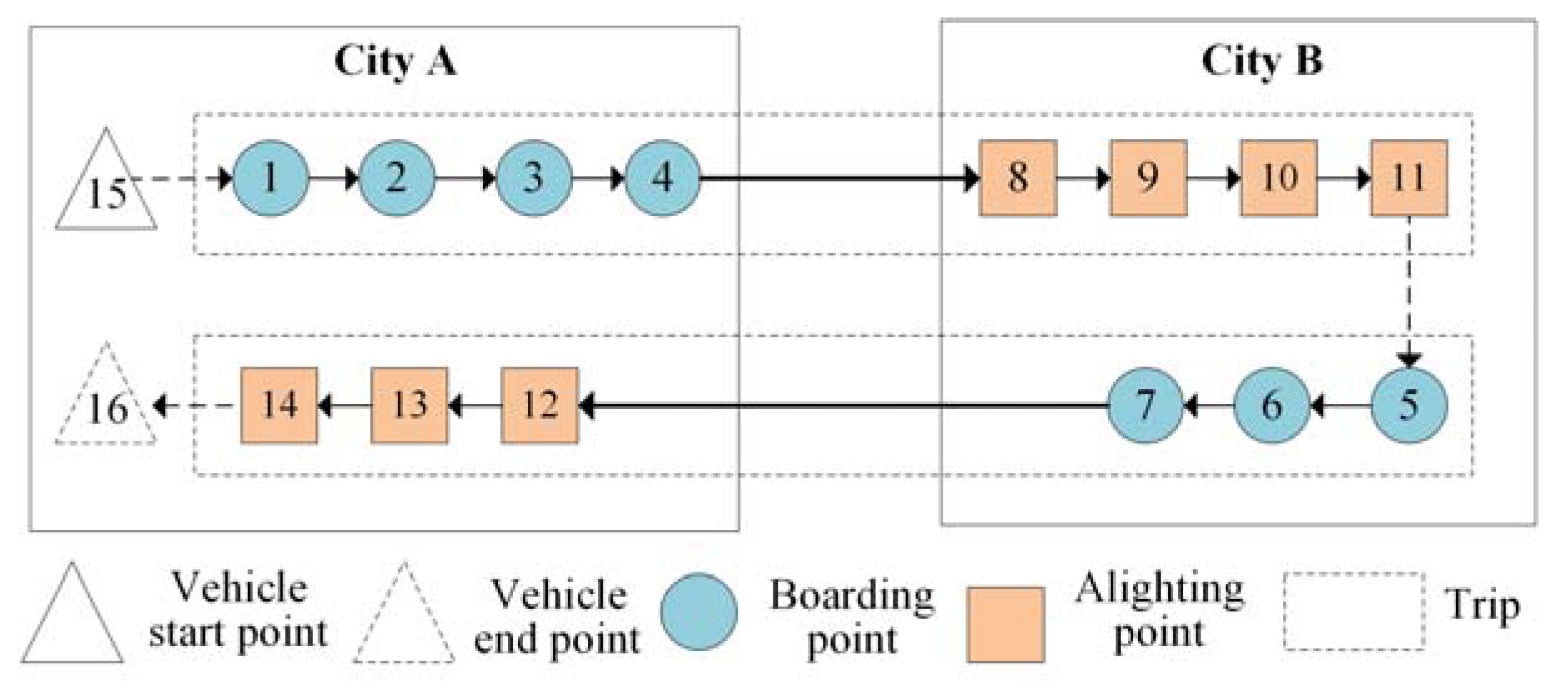
Intercity carpooling mainly includes four parts: platform, passengers, drivers, and government. The specific relationship is shown in Figure 1. Taking the carpooling between cities A and B as an example, it is assumed that there is a platform to provide carpooling services for the two cities. Travelers need to send carpooling demand to the platform in advance, including boarding and alighting points, time windows, etc. For travelers who cannot be served, the platform will inform them in advance. Therefore, this study is a static VRPTW [9]. The operation mode of intercity carpooling is to first pick up passengers from city A, and then transport them to city B. They cross the city, and boarding and alighting points appear in pairs.

It is assumed that the vehicle capacity is 4, and there is no empty driving between the two cities. There are two trips in Figure 2. Trip 1 is from city A to city B, and city A has one driver and four passengers. Trip 2 is from city B to city A, and city B has one driver and three passengers [2].

2.2. Assumptions

This paper is based on the following assumptions:

(1) The platform obtains the passengers boarding and alighting points, time window, etc. in advance according to the reservation information;

(2) Based on door-to-door transport, each boarding and alighting point has only one passenger;

(3) Using a single vehicle type, that is, the same passenger capacity of carpooling vehicles;

(4) Passengers can only drop off at the alighting point corresponding to the boarding point of the reservation information;

(5) Only considering the one-way operation from city A to city B, the vehicle does not return to the station after the operation, and the driving time and distance between the vehicle and the station are assumed to be 0;

(6) In good road conditions, the average speed of vehicles also remains constant;

(7) When the vehicle is served at each boarding and alighting point, the service time of each passenger is the same.

3. Model Construction

Notations and descriptions used in the model as shown in

Table A1. Notations and descriptions used in the model.

Sets	Definitions
V	Node set
A	Link set
P	Passenger demand point set
P+	Passenger boarding point number set
P−	Passenger alighting point number set
K	Vehicle set
Parameters	Descriptions
Z1	Passenger cost
Z2	Platform revenue
Z3	Carbon emission cost
C11	Passenger time cost in vehicle
C12	Passenger time cost outside vehicle
W1	Passenger waiting cost per unit time in vehicle
Tijk	Travelling time between point i and point j of vehicle k
WTik	Waiting time at point i of vehicle k
Ts	Average service time per passenger
Qi	Number of passengers in vehicle before arriving at point i
Tik	Arrival time at point i of vehicle k
FT0k	Vehicle departure time from the parking lot
W2	Passenger waiting cost per unit time outside vehicle
I	Platform income
C21	Fixed and variable costs of the platform
C22	Penalty cost of vehicle arriving later than time window
F	Fare for a single trip
W3	The fixed cost of a single trip
W4	Freeway toll per unit mileage
W5	Fuel consumption cost per unit mileage
dij	Distance between point i and point j
$V_{ij}^k$	Average speed between point i and point j
[ETi, LTi]	Time window at point i, ETi is the earliest arrival time and LTi is the latest arrival time
θ1	Penalty coefficient arriving later than time window
tik	Departure time of vehicle k from point i
f	Load limit of vehicle
w	Vehicle weight
fij	Real-time load
Pij	Fuel consumption between point i and point j
aij	Parameters related to links
β1	Parameters related to vehicle
ε	Carbon tax rate
δ	Fuel consumption factor
ε0	Fuel consumption rate at no-load
ε*	Fuel consumption rate at full load
$T_{\mathrm{i}}^{\max }$	Maximum travelling time for passenger at point i
Decision Variables	Definitions
Xijk	0–1 variable, Xijk = 1 if vehicle k travels from point i to point j; otherwise, Xijk = 0.
Xik	0–1 variable, Xik = 1 if the passenger at point i is transported by vehicle k; otherwise, Xik = 0.

. It is assumed that the platform can service up to n passengers with k cars. The vehicle set is $K=\left\{1,2,\cdots ,k\right\}$ and the vehicle is a 4-seater passenger car and can take up to 3 passengers. If the passenger gets on the car at the point i, he will get off at the point n + i corresponding to the boarding point. The passenger boarding point number set is $P^{+}=\left\{1,2,\cdots ,n\right\}$, and the alighting point number set is $P^{-}=\left\{n+1,n+2,\cdots ,2n\right\}$. So, the demand point set is.

The intercity carpooling path optimization can be described as a complete weighting graph $G\left(V,A\right)$ from the perspective of graph theory. $V=\left\{0,1,\cdots ,2n\right\}$ represents the node set, and 0 is the virtual parking lot, indicating the beginning and end of the trip. A represents the link set between points i and j.

3.1. Multi-Objective Function Determination

3.1.1. Passenger Perspective: Cost Minimization

Passenger cost includes passenger time cost in vehicle C₁₁, passenger time cost outside vehicle C₁₂, and fare for a single trip F. Passenger time cost in vehicle includes travelling time cost and waiting time cost at demand point, as shown in Equation (1)

$$C_{11}=W_1{\displaystyle \sum _{k\in K}{\displaystyle \sum _{i\in P}{\displaystyle \sum _{j\in P}{X}_{ijk}\left(T_{ijk}+W{T}_{ik}+T_s\right)}}\times Q_i}$$

(1)

where Q_i represents the number of passengers in vehicle before arriving at point i. The calculation is shown in Equation (2):

$$Q_i=\{\begin{array}{l}{\displaystyle \sum X_{ik}-1},\forall i\in P^{+},k\in K\\ {\displaystyle \sum X_{ik}+1,\forall i\in P^{-},k\in K}\end{array}$$

(2)

The waiting time is affected by the earliest arrival time, as shown in Equation (3):

$$W{T}_{ik}=\max \left[\left(E{T}_i-T_{ik}\right),0\right]$$

(3)

T_ik is arrival time at point i of vehicle k, as shown in Equation (4):

$$T_{ik}=F{T}_{0k}+{\displaystyle \sum _{i\in P^{+}}{\displaystyle \sum _{j\in \left\{0,1,\cdots ,i-1\right\}}\left(T_{jik}+T_s\right)}}$$

(4)

The waiting time cost of passengers at demand point is affected by the time window and vehicle service time at boarding point, as shown in Equation (5):

$$C_{12}=W_2{\displaystyle \sum _{k\in K}{\displaystyle \sum _{i\in p^{+}}\max \left(T_{ik}-L{T}_i,0\right)}}$$

(5)

3.1.2. Platform Perspective: Revenue Maximization

The platform revenue is income minus cost, and the income of the platform can be expressed as Equation (6):

$$I=F\times {\displaystyle \sum _{k\in K}{\displaystyle \sum _{i\in P}{X}_{ik}}}$$

(6)

Platform cost mainly includes fixed cost, variable cost, and penalty cost. The fixed cost consists of driver’s salary, vehicle depreciation fee, insurance maintenance fee etc. To simplify the analysis, a fixed value is taken according to the vehicle type. The variable cost consists of freeway toll and fuel cost as shown in Equation (7):

$$C_{21}=W_3+{\displaystyle \sum _{k\in K}{\displaystyle \sum _{i\in P}{\displaystyle \sum _{j\in P}\left(W_4+W_5\right)\times X_{ijk}\times d_{ij}}}}$$

(7)

If the vehicle arrives later than the passenger time window, there will be a certain penalty cost, as shown in Equation (8):

$$C_{22}=\{\begin{array}{ll}0\hspace{1em}\hspace{1em}& 0<T_{ik}\le L{T}_i\\ {\displaystyle \sum _{k\in K}{\displaystyle \sum _{\mathrm{i}\in P}{\theta }_1\times \frac{T_{ik}-L{T}_i}{L{T}_i-E{T}_i}}\hspace{1em}}& T_{ik}>L{T}_i\end{array}$$

(8)

3.1.3. Government Perspective: Carbon Emission Minimization

Because the greenhouse gas emissions of vehicles during driving are affected by many factors, it is very difficult to measure the greenhouse gases generated [16]. Carbon dioxide emissions are the main factors that aggravate the greenhouse effect. Thus, this paper only measures carbon emissions. A large number of studies have proven that carbon emissions are positively correlated with fuel consumption [25,26,27]. In order to facilitate the calculation, the fuel consumption is multiplied by the conversion factor to calculate carbon emissions. The fuel consumption model is based on the comprehensive fuel model constructed by Bektas et al. [28]. The model fully considers the influence of vehicle speed and load on vehicle fuel consumption. The load limit of vehicle is f, the vehicle weight is w, the real-time load is f_ij, and the fuel consumption expression is shown in Equation (9):

$$P_{ij}={\alpha }_{ij}\left(w+f_{ij}\right)d_{ij}+{\beta }_1{v}_{ij}^k{}^2{d}_{ij}$$

(9)

However, the model calculation data are too complicated, so the influence of load on fuel consumption is more specific. The fuel consumption rate of the vehicle at no-load and full load is ε₀ and ε*, respectively. The fuel consumption of the vehicle loads is shown in Equation (10):

$$S\left(f_{ij}\right)=\alpha \left(w+f_{ij}\right)+\beta$$

(10)

Assuming that the fuel consumption of the vehicle at no-load is ${\epsilon }_0=\alpha w+\beta$, and the fuel consumption at full load is ${\epsilon }^{*}=\alpha \left(w+f\right)+\beta$, then $\alpha =\frac{{\epsilon }^{*}-{\epsilon }_0}{f}$. Substituting into Equation (10) yields Equation (11):

$$S\left(f_{ij}\right)=\frac{{\epsilon }^{*}-{\epsilon }_0}{f}\left(w+f_{ij}\right)+\beta =\frac{{\epsilon }^{*}-{\epsilon }_0}{f}w+\beta +\frac{{\epsilon }^{*}-{\epsilon }_0}{f}{f}_{ij}={\epsilon }_0+\frac{{\epsilon }^{*}-{\epsilon }_0}{f}{f}_{ij}$$

(11)

The formula for calculating carbon cost by carbon tax method is Equation (12) by replacing the influence of load on vehicle fuel consumption in Equation (11) with Equation (9):

$$Z_3=\epsilon \times \delta \times {\displaystyle \sum _i{\displaystyle \sum _j{\displaystyle \sum _k\left({\epsilon }_0+\frac{{\epsilon }^{*}-{\epsilon }_0}{f}{f}_{ij}+{\beta }_1{V}_{ij}^k{}^2\right)d_{ij}{X}_{ijk}}}}$$

(12)

3.2. Multi-Objective Model Construction

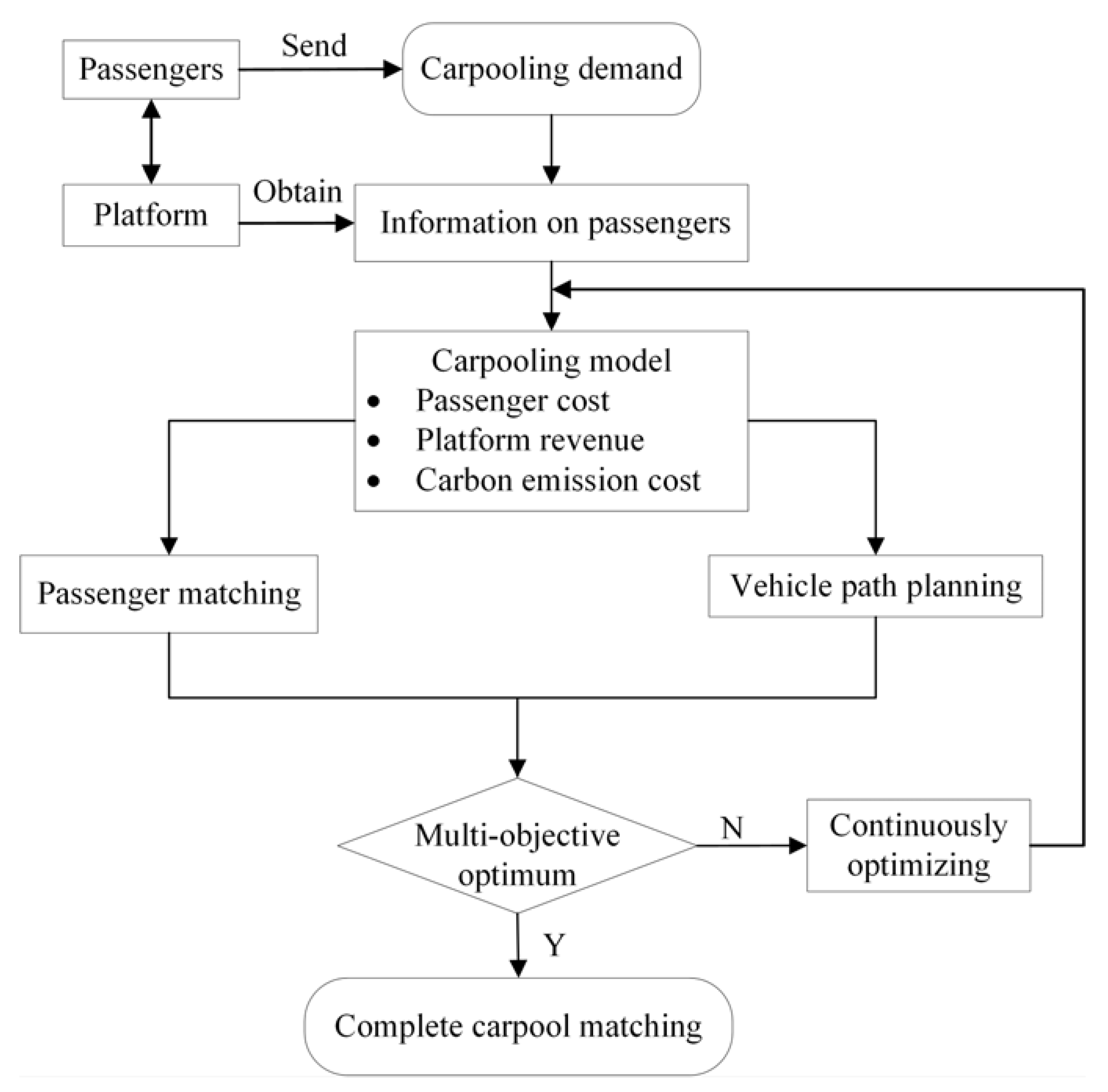
As shown in Figure 3, firstly, passengers send carpooling demand to the platform. Based on the obtained passenger information, the platform comprehensively considers passenger cost, platform revenue, and carbon emission cost for passenger matching and vehicle path planning to achieve multi-objective optimization.

Mathematically, this problem can be expressed as a multi-objective planning model.

Objective function:

$$Min{Z}_1=Min\left\{\begin{array}{l}{W}_1{\displaystyle \sum _{k\in K}{\displaystyle \sum _{i\in P}{\displaystyle \sum _{j\in P}{X}_{ijk}\left(T_{ijk}+\max \left[\left(E{T}_i-F{T}_{0k}-{\displaystyle \sum _{i\in P}{\displaystyle \sum _{j\in P}\left(T_{ijk}+T_s\right)}}\right),0\right]+T_s\right)}}}\times Q_i\\ +W_2{\displaystyle \sum _{k\in K}{\displaystyle \sum _{i\in p^{+}}\max \left(T_{ik}-L{T}_i,0\right)+F}}\end{array}\right\}$$

(13)

$$Max{Z}_2=Max\left\{F\times {\displaystyle \sum _{k\in K}{\displaystyle \sum _{i\in P}{X}_{ik}}}-W_3-{\displaystyle \sum _{k\in K}{\displaystyle \sum _{i\in P}{\displaystyle \sum _{j\in P}\left(W_4+W_5\right)\times X_{ijk}\times d_{ij}}}}-C_{22}\right\}$$

(14)

$$Min{Z}_3=Min\left\{\epsilon \times \delta \times {\displaystyle \sum _i{\displaystyle \sum _j{\displaystyle \sum _k\left({\epsilon }_0+\frac{{\epsilon }^{*}-{\epsilon }_0}{f}f+{\beta }_1{V}_{ij}^k{}^2\right)d_{ij}{X}_{ijk}}}}\right\}$$

(15)

Subject to:

$$1\le {\displaystyle \sum _{i\in P^{+}}{X}_{ik}}\le 3,\forall k\in K$$

(16)

$${\displaystyle \sum _{j\in P,j\ne i}{X}_{ijk}-}{\displaystyle \sum _{j\in P,j\ne n+i}{X}_{j,i+n,k}=0}, \forall i\in P^{+}$$

(17)

$${\displaystyle \sum _{k\in K}{\displaystyle \sum _{i\in P}{X}_{ijk}=1},\forall j\in P}$$

(18)

$${\displaystyle \sum _{j\in P}{X}_{ijk}\left(T_{ijk}+W{T}_{ik}+T_s\right)}\le T_{\mathrm{i}}^{\max },\forall i\in P^{+}$$

(19)

$$0<E{T}_i<L{T}_i\hspace{0.17em},\forall i\in P^{+}$$

(20)

$$X_{ijk}\in \left\{0,1\right\},\forall i,j\in P,k\in K$$

(21)

$$X_{ik}\in \left\{0,1\right\},\forall i\in P,k\in K$$

(22)

$$i,j,k\in N^{+}$$

(23)

where the objective function (13) represents the minimization of passenger cost; the objective function (14) represents the maximization of platform revenue; the objective function (15) represents the minimization of carbon emission cost; the constraint (16) is the vehicle capacity constraint, and the passenger capacity in the vehicle cannot exceed the maximum allowable passenger capacity; the constraint (17) is the boarding and alighting points constraint. If vehicle k serves passenger at point i, passenger will be picked up at boarding point i and transported to alighting point n + i; constraint (18) is the vehicle service constraint, indicating that e point i can only be served by vehicle k; constraint (19) is that the length of time for passengers to arrive at alighting point does not exceed the maximum travel time; constraint (20) is the time window constraint; the constraints (21) and (22) are the decision variable value constraints; the constraint (23) is non-negation.

4. Algorithm Design

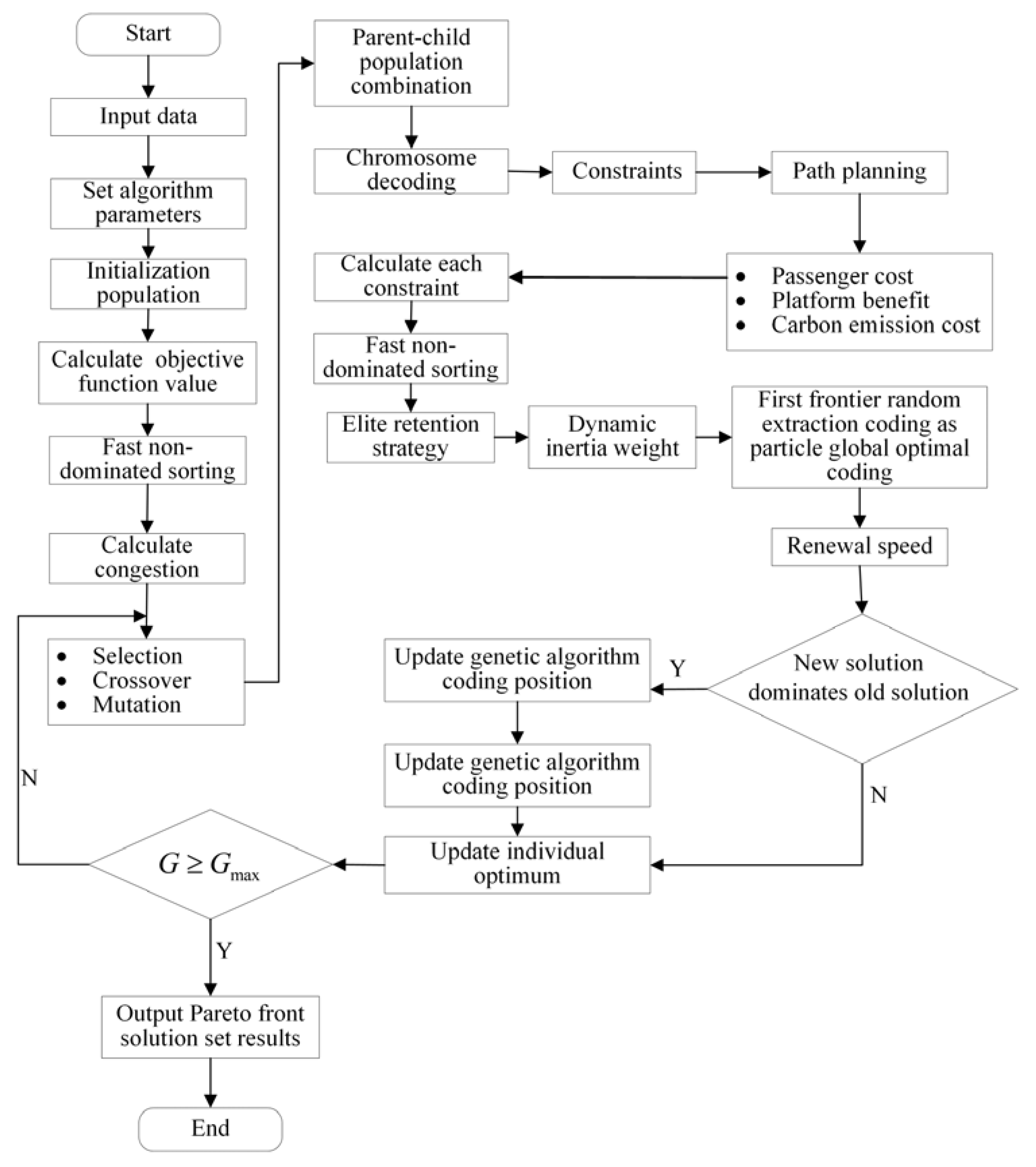
The PSO-NSGA-II algorithm is used to solve the multi-objective intercity carpooling problem. The particle swarm optimization algorithm is used to improve the operator to help the operator remember the previous search position and iterative information. It can improve the coordination ability between the operators and accelerate the search speed of the operator [19]. The overall process of the PSO-NSGA-II algorithm is shown in Figure 4.

(1)

Initialize population

First, the encoding of the vehicle–passenger assignment matrix is determined. It is usually a high-dimensional sparse matrix, so it is not appropriate to use binary matrix coding directly [18]. Especially in the design of crossover and mutation operation, the operation efficiency is very low, and most of the operation is invalid. Therefore, the coding method based on natural number fixed length is adopted, and the full arrangement of passenger boarding point numbers is used to represent the solution vector of the carpooling line. O and D represent the freeway entrances and exits of the origin and destination cities. The chromosome is composed of passenger demand points, vehicle intervals, and high-speed entrances and exits, ensuring that each passenger is served only once by one vehicle and all passengers are served. By examining the vehicle capacity constraints and the boarding and alighting point constraints, the full arrangement is cut to form a specific carpooling line. Figure 5 randomly generates an initial population of scale.

(2)

Fast non-dominated sorting

The population individuals are stratified according to the level of non-inferior solutions. Firstly, the non-dominated solution set of the population is found, which is placed in the first non-dominated layer and given a non-dominated sequence $i_{rank}=1$. Then, the assigned individuals are removed from the population, and the new non-dominated solution set is continued to be found. It is placed in the second non-dominated layer and given a non-dominated sequence $i_{rank}=2$. The above process is performed in turn, and the entire population is traversed until the entire population is stratified.

(3)

Crowded degree sorting

The distance between the individuals located in the same layer is initialized, that is $L{\left[i\right]}_d=0$, and the individuals in this layer are arranged according to the value of the objective function m. The individual crowded distance located on the edge of the sorting edge is given infinite, that is $L{\left[0\right]}_d=L{\left[i\right]}_d=\infty$. For the individuals in the middle, the crowding distance is $L{\left[i\right]}_d=L{\left[i\right]}_d+\left(L{\left[i+1\right]}_m+L{\left[i-1\right]}_m\right)/\left(Z_m^{\max }-Z_m^{\min }\right)$. $L{\left[i+1\right]}_m$ and $L{\left[i-1\right]}_m$ are the values of the objective function $m$ of the $i+1$ and $i-1$ individuals in the layer. $Z_m^{\max }$ and $Z_m^{\min }$ are the maximum and minimum values of the objective function $m$ in the layer. Repeat the above calculation for each objective function to obtain the crowding distance of the individual.

(4)

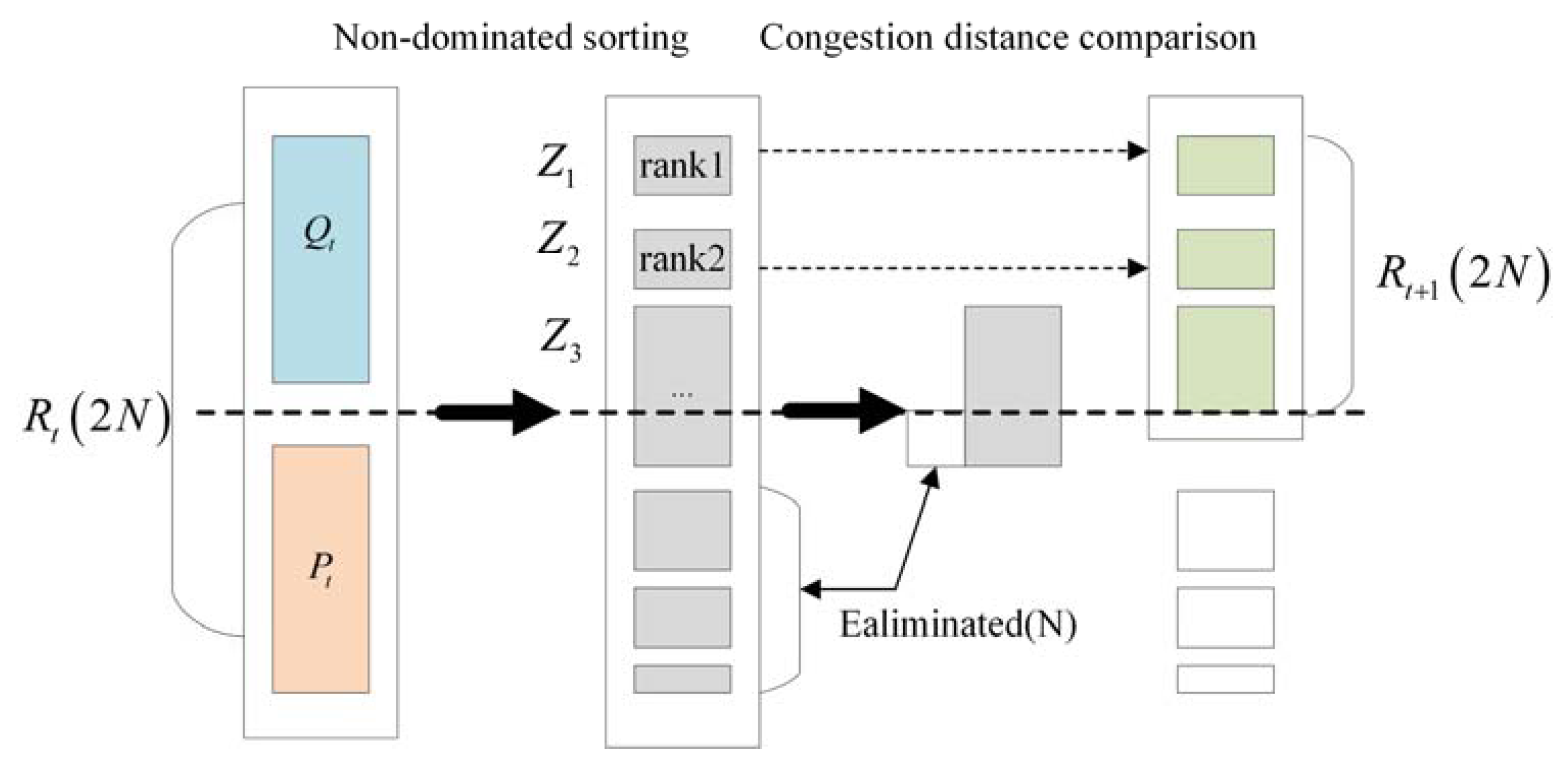
Elite retention strategy

Q_t is the child population, P_t is the parent population, and N is the set population size. The specific implementation of the elitist retention strategy is as follows.

Step 1: The individuals in the parent population and the individuals in the child population are merged and reorganized together to obtain a new population. The individuals in the new population are sorted from small to large according to the non-dominated level, and multiple non-dominated level sequences are obtained.

Step 2: The individuals in each non-dominated level sequence are sorted from large to small according to the individual crowding degree, so as to realize the sorting of the individuals in the new population.

Step 3: We choose to retain the previous individual in the new population into the next generation population.

The specific operation steps are shown in Figure 6.

(5)

Improved particle swarm optimization operator

Step 1: Set the parameters: the maximum inertia factor w_max, the minimum inertia factor w_min, the current number of iterations G, and the maximum iteration times G_max. The inertia weight w is calculated according to Equation (24):

$$w=w_{\max }-\frac{w_{\max }-w_{\min }}{G_{\max }}\times G$$

(24)

Step 2: Assuming that the coordinate position of each particle is $x_i=\left(x_{i1},x_{i1},\cdots x_{in}\right)$, and the velocity corresponding to each particle is $v_i=\left(v_{i1},v_{i2},\cdots v_{in}\right)$. The historical optimal value searched by the particle itself is $p_i=\left(p_{i1},p_{i2},\cdots p_{in}\right)$, and the historical optimal value searched by all particles is $p_m=\left(p_{m1},p_{m2},\cdots p_{mn}\right)$. The velocity of the particle is updated according to Equation (25):

$$v_{id}^{k+1}=w{v}_{id}^k+c_1\xi \left(p_{id}^k-x_{id}^k\right)+c_2\eta \left(p_{md}^k-x_{id}^k\right)$$

(25)

where ξ and η are random numbers uniformly distributed in the interval [0, 1]. i is particle, k is generation, and d is dimension. $v_{id}^k$ represents the velocity, $x_{id}^k$ represent the position, $p_{id}^k$ represents the individual optimal position, and $p_{md}^k$ represents the global optimal position. w can maintain the original velocity of the particle. c₁ represents the weight coefficient of the particle tracking its historical optimal value, that is the particle’s understanding of itself. c₂ represents the weight coefficient of the particle tracking the historical optimal value of the group, that is the particle’s understanding of the whole group.

Step 3: Update the particle position according to Equation (26):

$$x_{id}^{k+1}=x_{id}^k+v_{id}^{k+1}$$

(26)

If the solution corresponding to the new position generated by the particle update can dominate the solution corresponding to the original position, the original solution is replaced by the newly generated solution.

5. Example Analysis

5.1. Data Source

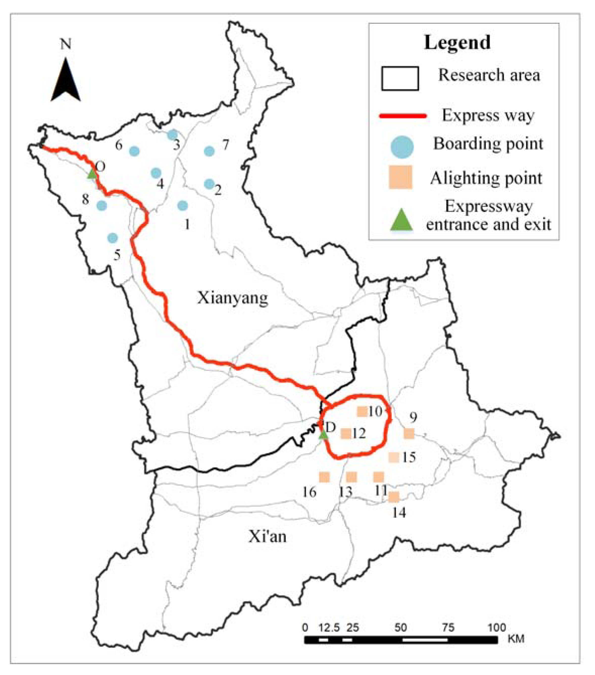
This paper selects the carpooling examples of Xi’an and Xianyang in Shaanxi Province to verify the effectiveness of this method. As shown in Figure 7, the main freeways between the two cities are the Ring Expressway and G70. The original map data of the road network are derived from the OpenStreetMap, processed and vectorized by ArcGIS 10.7 software.

(1)

Passenger information

We assume that there are 3 cars serving 8 passengers, and Xianyang City is origin and Xi’an City is destination. This paper obtains the longitude and latitude coordinates of each boarding and alighting point through the open platform of network map, as shown in

Table 1. Passenger information.

Boarding Point	Longitude and Latitude	Alighting Point	Longitude and Latitude	Time Window [ETi, LTi]/min	Maximum Travelling Time ${\mathit{T}}_{\mathbf{i}}^{\mathbf{max}}$/min
1	(108.24, 35.05)	9	(109.12, 34.21)	[15, 20]	50
2	(108.36, 35.06)	10	(108.94, 34.32)	[15, 20]	55
3	(108.26, 35.22)	11	(108.88, 34.10)	[10, 15]	55
4	(108.15, 35.12)	12	(108.89, 34.26)	[20, 25]	60
5	(108.01, 34.93)	13	(108.78, 34.11)	[20, 25]	55
6	(108.08, 35.19)	14	(109.01, 34.06)	[10, 15]	60
7	(108.36, 35.13)	15	(109.04, 34.15)	[5, 10]	45
8	(107.94, 35.03)	16	(108.71, 34.14)	[25, 30]	65

. The coordinates of the entrance and exit of the expressway are O (107.94, 35.11) and D (108.79, 34.25) respectively.

(2)

Node distance

According to the traffic network between the two points, the distance is shown in

Table 2. Distance matrix/km.

	1	2	3	4	5	6	7	8	…
1	0	3.45	6.39	4.12	8.23	7.21	4.72	9.32	…
2	3.45	0	6.53	6.80	11.49	9.67	2.68	12.77	…
3	6.39	6.53	0	4.96	13.07	5.78	4.35	12.22	…
4	4.12	6.80	4.96	0	8.21	3.09	6.47	7.35	…
5	8.23	11.49	13.07	8.21	0	9.57	12.90	4.06	…
6	7.21	9.67	5.78	3.09	9.57	0	8.81	7.31	…
7	4.72	2.68	4.35	6.47	12.90	8.81	0	13.41	…
8	9.32	12.77	12.22	7.35	4.06	7.31	13.41	0	…
…	…	…	…	…	…	…	…	…	…

Note: The number represents the boarding and alighting points.

.

(3)

Parameters value

To solve the example, the numerical values of the parameters required in the model are shown in

Table 3. Parameter value.

Parameter	Description	Value
W1	Passenger waiting cost per unit time in vehicle (RMB(USD)/min)	0.2
W2	Passenger waiting cost per unit time outside vehicle (RMB(USD)/min)	0.4
W3	The fixed cost of a single trip (RMB(USD))	10
W4	Freeway toll per unit mileage (RMB(USD)/km)	0.3
W5	Fuel consumption cost per unit mileage (RMB(USD)/km)	0.5
F	Fare for a single trip (RMB(USD))	30
Ts	Average service time per passenger (min)	1
θ1	Penalty coefficient arriving later than the time window	0.2
$V_{ij}^k$	The average speed between point i and point j (km/h)	50
w	Vehicle weight (kg)	1500
fij	Real-time load (kg)	100
ε	Carbon tax rate (RMB(USD)/t)	5
δ	Fuel consumption factor	2.544
ε0	Fuel consumption rate at no-load	0.254
ε*	Fuel consumption rate at full load	0.276

.

5.2. Results and Discussion

In the example, there are 3 vehicles and 8 passenger demand points. The parameters involved in the model are imported into the designed Python 3 program. The algorithm parameters are set as follows: initial population size $P=50$, crossover probability $P_c=0.8$, mutation probability $P_m=0.1$, the maximum inertia factor $w_{\max }=0.9$, the minimum inertia factor $w_{\min }=0.8$, the weight coefficient of the particle tracking its historical optimal value $c_1=1.5$, the weight coefficient of the particle tracking the historical optimal value of the group $c_2=1.2$, the number of iterations terminated $G_{\max }=100$.

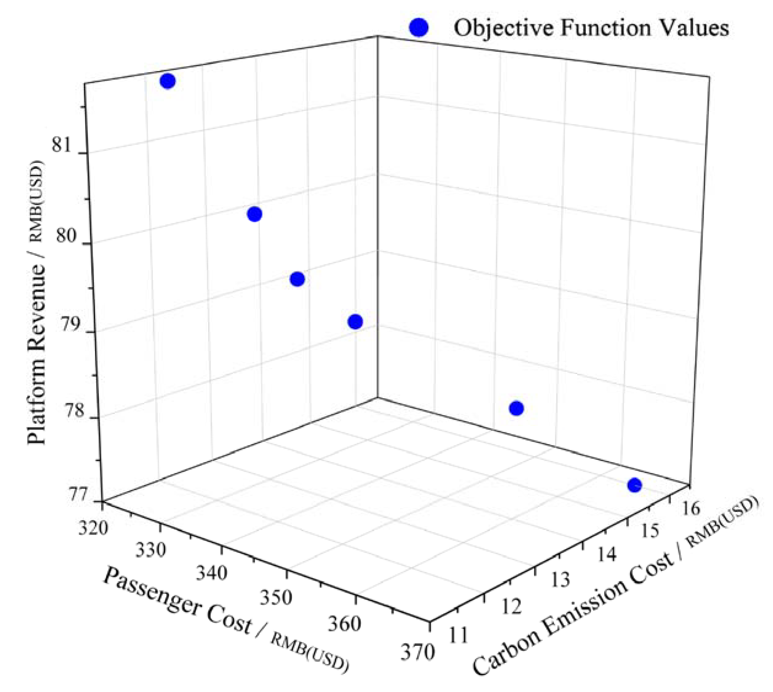
The Pareto iterates 100 times and the Pareto frontier graph is shown in Figure 8.

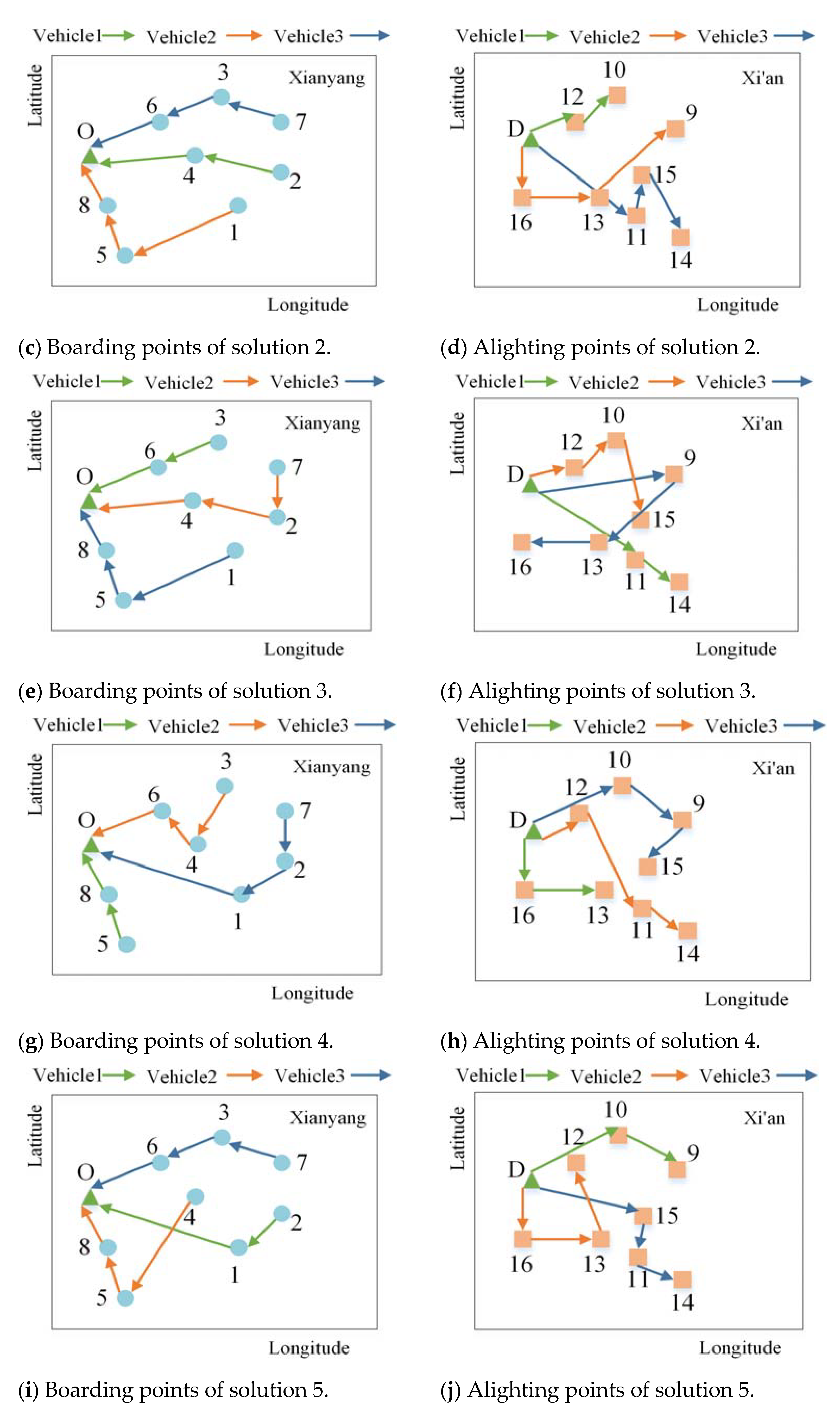
There are six non-dominated solutions, which together constitute the Pareto optimal solution set. The details of the six non-dominated solutions are shown in

Table 4. Sets of non-dominant solutions.

Number of Non-Dominated Solutions	Passenger Cost /RMB (USD)	Platform Revenue /RMB (USD)	Carbon Emission Cost/RMB (USD)
1	325.68	81.75	11.8
2	328.25	80.26	12.8
3	334.75	79.52	13.5
4	342.13	79.81	13.2
5	355.64	78.64	14.8
6	365.58	77.52	15.7

.

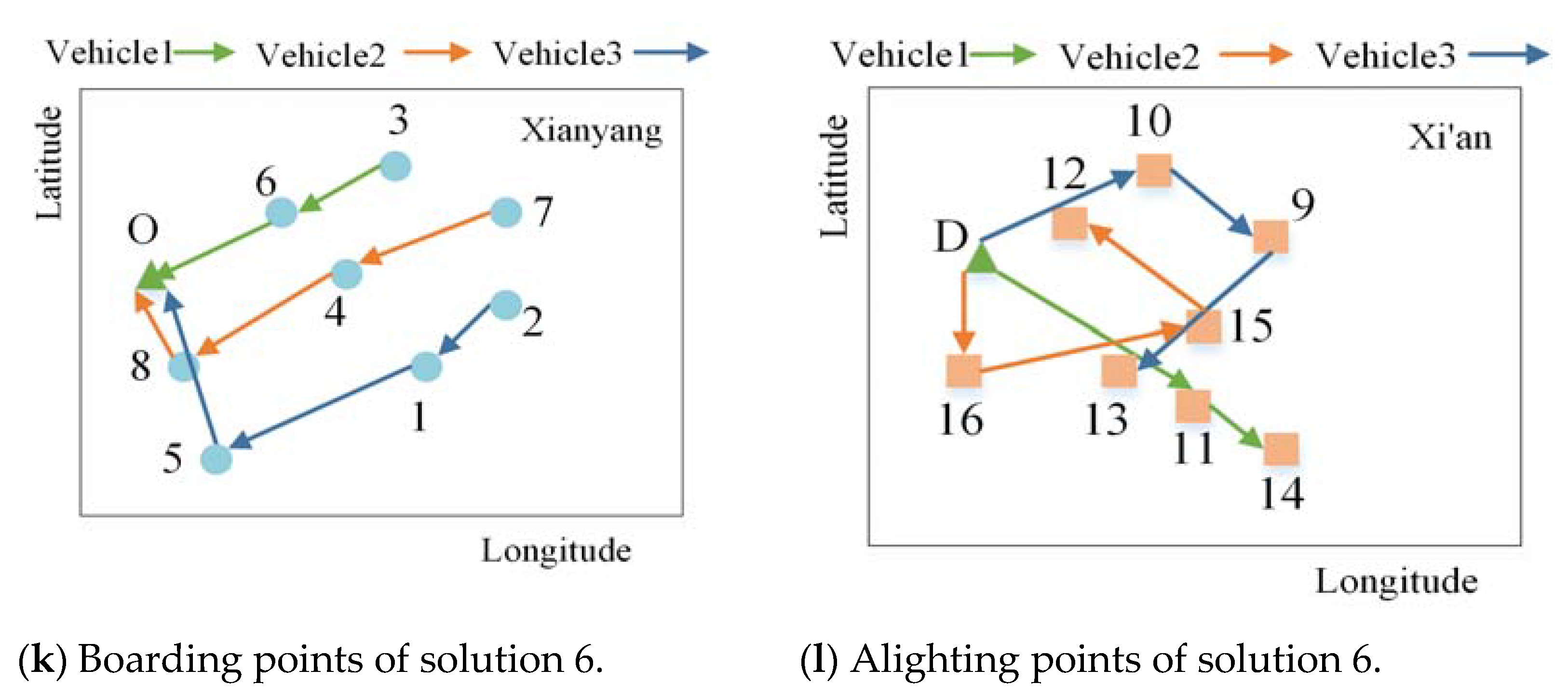
The vehicle route corresponding to each non-dominated solutions is shown in the Figure 9.

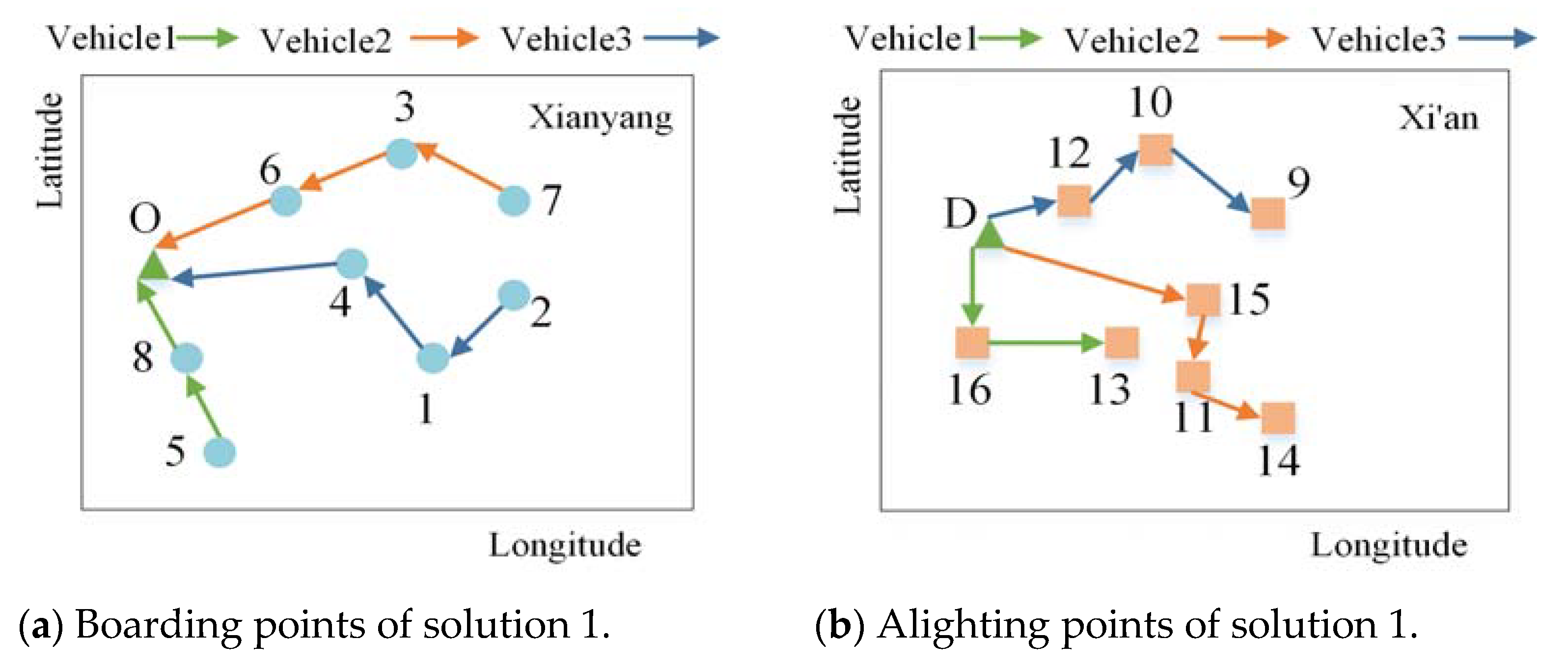
Considering the objective function, the optimal solution to this problem is selected in the Pareto optimal solution set 1. The passenger cost is RMB(USD) 325.68, the platform revenue is RMB(USD) 81.75, and the carbon emission cost is RMB(USD) 11.80. The results of intercity carpool route optimization are shown in

Table 5. Model solution results.

Vehicle Number	Path	Travel Time (min)	Passenger Cost/RMB (USD)	Platform Revenue/RMB (USD)	Carbon Emission Cost/RMB (USD)
Vehicle 1	5-8-O-D-16-13	59.08	75.26	14.58	3.39
Vehicle 2	7-3-6-O-D-15-11-14	81.60	126.15	28.32	4.36
Vehicle 3	2-1-4-O-D-12-10-9	72.35	124.27	38.85	4.05
Total		213.03	325.68	81.75	11.80

. The path of vehicle 1 is 5-8-O-D-16-13, the path of vehicle 2 is 7-3-6-O-D-15-11-14, and the path of vehicle 3 is 2-1-4-O-D-12-10-9. Vehicle 2 has the longest driving time of 81.60 min, and vehicle 1 has the shortest driving time of 59.08 min. The vehicle driving path is shown in Figure 10.

During the 100 iterations of the algorithm, it will gradually converge. The three objective functions established in the model will gradually stabilize with the increase in the number of iterations. To verify the performance of the PSO-NSGA-II algorithm proposed in this paper, the NSGA-II algorithm is used to solve the problem. The numerical change process of the objective function is shown in Figure 11.

As for passenger cost iteration curve in Figure 11a, the NSGA-II algorithm converges to RMB(USD) 330.25 around the 50th generation. The PSO-NSGA-II algorithm has a significantly higher decline rate than the NSGA-II algorithm. It begins to converge around the 40th generation and converges to RMB(USD) 325.68, which is RMB(USD) 4.57 lower than that.

Platform revenue iteration curve in Figure 11b, the PSO-NSGA-II algorithm and the NSGA-II algorithm begin to converge at about 50 generations, and converge at RMB(USD) 81.75 and RMB(USD) 80.14 respectively. Therefore, the optimal solution of the PSO-NSGA-II algorithm is better than that of the NSGA-II algorithm

Carbon emission cost iterative curve in Figure 11c, the PSO-NSGA-II algorithm began to decline at a faster rate, tended to be flat after 5 iterations, and converged to RMB(USD) 11.80 around the 60th generation. The NSGA-II algorithm fluctuated greatly in the first 10 iterations, then tended to be flat, and converged to RMB(USD) 12.15 around the 50th generation. In summary, the PSO-NSGA-II algorithm is superior to the NSGA-II algorithm in both convergence speed and convergence value, so the algorithm proposed in this study is effective.

6. Conclusions

This paper defines the intercity carpooling path optimization problem with time window. Firstly, based on the passenger-platform-government perspective, a multi-objective optimization model of intercity carpooling considering carbon emissions is constructed. The three objective functions are the minimization of passenger cost, the maximization of platform revenue and the minimization of carbon emission cost, and the constraints are vehicle capacity, boarding and alighting points and vehicle services. Secondly, in order to further improve the coordination ability and search speed of the operator, the PSO-NSGA-II algorithm is designed to solve the model by using the particle swarm optimization algorithm to help the operator to memorize the previous search position and iterative information. Finally, taking Xi’an–Xianyang intercity carpooling as an example, the validity of the model and algorithm is verified.

In the example, the PSO-NSGA-II algorithm is used to obtain six non-dominated solution sets. In the case of comprehensive consideration of the objective function, the optimal solution of this problem is selected. Passenger cost is RMB(USD) 325.68, platform revenue is RMB(USD) 81.75, and carbon emission cost is RMB(USD) 11.80. The corresponding intercity carpool path optimization results: the path of vehicle 1 is 5-8-O-D-16-13, the path of vehicle 2 is 7-3-6-O-D-15-11-14, and the path of vehicle 3 is 2-1-4-O-D-12-10-9. Compared with the NSGA-II algorithm, the passenger cost obtained by the PSO-NSGA-II algorithm proposed in this paper is reduced by RMB(USD) 4.57, the platform revenue is increased by RMB(USD) 1.61, the carbon emission cost is reduced by RMB(USD)0.35, and the convergence speed is also significantly better than the NSGA-II algorithm.

However, this study still has shortcomings. It only verifies the effectiveness of the model and algorithm. The research on the impact of model parameter changes on the results is insufficient. The next step can focus on the impact of fare changes, government subsidies, and platform cost increases on the optimal solution.

References

1. CIR. China Intercity Travel Industry Present Situation Investigation and Future Development Trend Analysis Report. 2022. Available online: https://www.cir.cn/7/33/ChengJiChuXingHangYeXianZhuangYu.html (accessed on 10 January 2023).
2. Rey-Merchán, M.D.C.; López-Arquillos, A.; Pires Rosa, M.; Gómez-de-Gabriel, J.M. Proposal for an institutional carpooling system among workers from the public-education sector. Sustainability 2022, 14, 14601. [Google Scholar] [CrossRef]
3. Liu, X.; Yan, X.; Liu, F.; Wang, R.; Leng, Y. A trip-specific model for fuel saving estimation and subsidy policy making of carpooling based on empirical data. Appl. Energy 2019, 240, 295–311. [Google Scholar] [CrossRef]
4. Dantzig, G.B.; Ramser, J.H. The truck dispatching problem. Manag. Sci. 1959, 6, 80–91. [Google Scholar] [CrossRef]
5. Sabar, N.R.; Bhaskar, A.; Chung, E.; Turky, A.; Song, A. A self-adaptive evolutionary algorithm for dynamic vehicle routing problems with traffic congestion. Swarm Evol. Comput. 2019, 44, 1018–1027. [Google Scholar] [CrossRef]
6. He, Y.; Wang, X.; Zhou, F.; Lin, Y. Dynamic vehicle routing problem considering simultaneous dual services in the last mile delivery. Kybernetes 2020, 49, 1267–1284. [Google Scholar] [CrossRef]
7. Bruglieri, M.; Mancini, S.; Pezzella, F.; Pisacane, O. A new mathematical programming model for the green vehicle routing problem. Electron. Notes Discret. Math. 2016, 55, 89–92. [Google Scholar] [CrossRef] [Green Version]
8. Solomon, M.M.; Desrosiers, J. Time window constrained routing and scheduling problems. Transp. Sci. 1988, 22, 1–13. [Google Scholar] [CrossRef] [Green Version]
9. Truden, C.; Maier, K.; Armbrust, P. Decomposition of the vehicle routing problem with time windows on the time dimension. Transp. Res. Procedia. 2022, 62, 131–138. [Google Scholar] [CrossRef]
10. Wang, Y.; Zhe, J.; Wang, X.; Sun, Y.; Wang, H. Collaborative multidepot vehicle routing problem with dynamic customer demands and time windows. Sustainability 2022, 14, 6709. [Google Scholar] [CrossRef]
11. Schaap, H.; Walther, G.; Schiffer, M.; Schneider, M. A large neighborhood search for the vehicle routing problem with multiple time windows. Transp. Sci. 2022, 56, 1369–1392. [Google Scholar] [CrossRef]
12. Zhang, M.; Wang, N.; He, Z.; Yang, Z.; Guan, Y. Bi-Objective vehicle routing for hazardous materials transportation with actual load dependent risks and considering the risk of each vehicle. IEEE Trans. Eng. Manag. 2019, 66, 429–442. [Google Scholar] [CrossRef]
13. Liu, X.; Titheridge, H.; Yan, X.; Wang, R.; Tan, W.; Chen, D.; Zhang, J. A passenger-to-driver matching model for commuter carpooling: Case study and sensitivity analysis. Transp. Res. Part C Emerg. Technol. 2020, 117, 102702. [Google Scholar] [CrossRef]
14. De Carvalho, V.R.; Golpayegani, F. Satisfying user preferences in optimised ridesharing services: A multi-agent multi-objective optimisation approach. Appl. Intell. 2022, 52, 11257–11272. [Google Scholar] [CrossRef]
15. Ma, N.; Zeng, Z.; Wang, Y.; Xu, J. Balanced strategy based on environment and user benefit-oriented carpooling service mode for commuting trips. Transportation 2021, 48, 1241–1266. [Google Scholar] [CrossRef]
16. Asghari, M.; Al-e-hashem, S.M.J.M.; Rekik, Y. Environmental and social implications of incorporating carpooling service on a customized bus system. Comput. Oper. Res. 2022, 142, 105724. [Google Scholar] [CrossRef]
17. Shen, J.; Liu, K.; Ma, C.; Zhao, Y.; Shi, C. Bibliometric analysis and system review of vehicle routing optimization for emergency material distribution. J. Traffic Transp. Eng. 2022, 9, 893–911. [Google Scholar] [CrossRef]
18. Beed, R.S.; Biswas, S.D.; Biswas, S.; Sarkar, S.; Roy, A. A hybrid multi-objective carpool route optimization technique using genetic algorithm and A* algorithm. Comput. Res. Model. 2021, 13, 67–85. [Google Scholar] [CrossRef]
19. Hsieh, F.S.; Zhan, F.M.; Guo, Y.H. A solution methodology for carpooling systems based on double auctions and cooperative coevolutionary particle swarms. Appl. Intell. 2019, 49, 741–763. [Google Scholar] [CrossRef]
20. Huang, S.C.; Lin, J.J.; Jiau, M.K. Global and local pareto optimality in coevolution for solving carpool service problem with time windows. IEEE Trans. Intell. Transp. Syst. 2020, 21, 934–946. [Google Scholar] [CrossRef]
21. Yu, Y.; Wang, S.; Wang, J.; Huang, M. A branch-and-price algorithm for the heterogeneous fleet green vehicle routing problem with time windows. Transp. Res. Part B Methodol. 2019, 122, 511–527. [Google Scholar] [CrossRef]
22. Wu, X.; Wang, L.; Chen, B.; Feng, Z.; Qin, Y.; Liu, Q.; Liu, Y. Multi-objective optimization of shield construction parameters based on random forests and NSGA-II. Adv. Eng. Inform. 2022, 54, 101751. [Google Scholar] [CrossRef]
23. Brahami, M.A.; Dahane, M.; Souier, M.; Sahnoun, M. Sustainable capacitated facility location/network design problem: A Non-dominated Sorting Genetic Algorithm based multiobjective approach. Ann. Oper. Res. 2022, 311, 821–852. [Google Scholar] [CrossRef]
24. Wang, Y.; Zhou, J.; Zhe, J.; Sun, Y.; Wang, X.; Wang, H. Electric vehicle charging Station location-routing problem with time windows and resource sharing. Sustainability 2022, 14, 11681. [Google Scholar] [CrossRef]
25. Xu, A.; Chen, J.; Liu, Z. Exploring the effects of carpooling on travelers’ behavior during the COVID-19 pandemic: A case study of metropolitan city. Sustainability 2021, 13, 11136. [Google Scholar] [CrossRef]
26. Guan, D.; Cong, X.; Li, J.; Wang, P.; Yang, Z.; Jing, X. Theoretical modeling and optimal matching on the damping property of mechatronic shock absorber with low speed and heavy load capacity. J. Sound Vibr. 2022, 535, 117113. [Google Scholar] [CrossRef]
27. Guan, D.; Pan, B.; Chen, Z.; Li, J.; Shen, H.; Pang, H. Quantitative modeling and bio-inspired optimization the clamping load on the bipolar plate in PEMFC. Energy 2023, 263, 125951. [Google Scholar] [CrossRef]
28. Bektaş, T.; Lapote, G. The pollution-routing problem. Transp. Res. Part B Methodol. 2011, 45, 1232–1250. [Google Scholar] [CrossRef]
Figure 1. Intercity carpooling mode.
Sustainability 15 02261 g001
Figure 2. An intercity carpooling example.(Note: The number represents the boarding and alighting points).
Sustainability 15 02261 g002
Figure 3. Diagram of carpooling matching steps.
Sustainability 15 02261 g003
Figure 4. Flowchart of PSO-NSGA-II algorithm.
Sustainability 15 02261 g004
Figure 5. Chromosome encoding and decoding.
Sustainability 15 02261 g005
Figure 6. Elite retention strategy.
Sustainability 15 02261 g006
Figure 7. Research area map.
Sustainability 15 02261 g007
Figure 8. Pareto frontier graph.
Sustainability 15 02261 g008
Figure 9. Vehicle routing diagram of all non-dominant solutions.
Sustainability 15 02261 g009aSustainability 15 02261 g009bSustainability 15 02261 g009c
Figure 10. Vehicle routing diagram.
Sustainability 15 02261 g010
Figure 11. Iteration curve diagram.
Sustainability 15 02261 g011