Abstract
Building energy consumption accounts for about 40% of global primary energy use and 30% of worldwide greenhouse gas (GHG) emissions. Among the energy-related factors present in buildings, heating, cooling, and air-conditioning (HVAC) systems are considered major contributors to whole-building energy use. To improve the energy efficiency of HVAC systems and mitigate whole-building energy consumption, accurately predicting the building energy consumption can play a significant role. Although many prediction approaches are available for building energy use, a machine learning-based modeling approach (i.e., black box models) has recently been considered to be one of the most promising building energy modeling techniques due to its simplicity and flexibility compared to physics-based modeling techniques (i.e., white box models). This study presents a building energy load forecasting method based on long-term short-term memory (LSTM) and transfer learning (TL) strategies. To implement this approach, this study first conducted raw data pre-processing analysis to generate input datasets. A hospital building type was considered for a case study in the first stage. The hospital prototype building model, developed by the U.S. department of energy (DOE), was used to generate an initial input training and testing dataset for source domain tasks before the transfer learning process. For the transfer learning process in a target domain, a simulation-based analysis was also conducted to obtain target datasets by assuming limited data lengths in different weather conditions. The training and testing procedures were performed using separate cooling and heating periods with and without the transfer learning process for source and target domain tasks, respectively. Lastly, a comparative analysis was carried out to investigate how the accuracy of LSTM prediction can be enhanced with the help of transfer learning strategies. The results from this study show that the developed LSTM-TL model can achieve better performance than the prediction model, which only uses LSTM under different weather conditions. In addition, accurate performance can vary according to different transfer learning methods with frozen and fine-tuning layers and locations.
1. Introduction
Buildings make up 40% and 30% of the global primary energy use and greenhouse gas emissions, respectively [1]. As buildings are major contributors to global energy use and environmental issues, enhancing energy efficiency and energy savings in buildings has been imperative recently worldwide. Among the energy use factors present in buildings, lighting, cooling, and heating have been the primary energy consumers for residential and commercial buildings, according to the US EIA [2]. Achieving high energy-efficiency in buildings requires that engineers understand the dynamic thermal behaviors of buildings with non-stationary environments and occupants [3]. According to the ASHRAE green guide report [4], understanding the energy sources and flows is crucial for identifying major aspects of building energy operations with the most significant energy-saving opportunities. This report [4] also represents a breakdown of commercial buildings’ energy use. The investigation shows that space heating and cooling, lighting, ventilation, plug-load, and water heating make up 70% and 87% of average energy end-use for US and European buildings, respectively. Such aspects are crucial for setting appropriate energy use goals and target savings. There are various energy-related technologies for achieving high energy efficiency in buildings, including both passive and active system measures [5]. For an example of a passive system, Kim et al. [6] investigated the thermal and daylighting effects of a double skin façade passive system by comparing interior and exterior blinds on building energy use. This comparative analysis was carried out based on simulated data from EnergyPlus. For an example of an active system, Kim et al. [7] evaluated the performance of variable refrigerant flow and rooftop variable air volume systems in simulation-based analysis. Based on their conclusions, advanced energy-related technologies could save building cooling, heating, and lighting consumption and improve entire-building energy efficiency and performance.
To achieve the greatest possible energy reductions, energy modeling needs to be considered to appropriately predict building energy consumption and behavior during the early stages of the design and maintenance processes after the completion of building construction [4]. The modeling techniques used to predict building thermal load and energy end-use can be broken down into three categories: white box, gray box, and black box models [8]. Engineers can adopt these prediction techniques to predict thermal and electric energy use patterns and investigate interacting behaviors between buildings and their connected energy systems during their analysis processes [9]. The physics-based methods (i.e., white box models) are based on physical principles and are used to calculate thermal and energy flows. In contrast, gray box models are known as semi-physical or hybrid models and work by combining the physics-based model with data-driven modeling approaches. The data-driven models (i.e., black box models) are good alternatives to implementing recent building energy prediction technologies, as building energy data is becoming more accessible and abundant [10]. Accurately predicting the demands affected by a building’s diverse factors with nonlinear and uncertain temporal patterns is challenging. However, the rapid development of smart sensors and devices for big data collection has led to the acceleration of data-driven model adaptation for thermal load and energy prediction in buildings [11]. Because of their flexibility, simplicity, and relative ease of access, such prediction models have recently gained much attention. Many algorithms and models have been developed to predict and analyze building energy demands and their patterns [12]. In general, building energy prediction algorithms can be classified into statistical analysis and artificial intelligence models. Statistical models estimate a building’s thermal aspects by reflecting the basis of linear regression analysis. Common statistical models include autoregressive integrated moving averages (ARIMA), multiple linear regression (MLR), and autoregressive with exogenous inputs (ARX) models [13]. Although statistical models are relatively simple for practical applications, it can be challenging for those models to detect abrupt changes and nonlinear relationships with overly complicated system configurations, such as the energy-related systems in a building [14]. To deal with such complexities in an easier manner, artificial intelligence (AI) models have been applied to building thermal load prediction and the analysis of building energy use.
Among available AI methods, machine learning (ML)-based models have become one of the most frequently used approaches for complex prediction problems due to their strong self-learning ability and nonlinear fitting ability [15]. The most common ML models include artificial neural networks (ANN), support vector machines (SVM), and random forests (RF). ANN has been explored extensively in the existing studies because of its ability to handle and generalize data, its ease of use, and the vast support present in software libraries [16]. Cox et al. [17] developed an ANN-based novel approach to predict building thermal load and determine the control strategy of thermal energy storage. Their results showed that the optimal control scheme with ANN-based thermal load prediction could effectively adapt to varying thermal loads and electricity prices to reduce cooling operation costs. Afram et al. [18] provided an overview of ANN-based model predictive control techniques. They concluded that determining the appropriate ANN architecture was crucial to performing better thermal prediction and designing the supervisory model predictive system control scheme. The taxonomy of a data-driven algorithm can be varied based on the criteria of a dataset for ANN architecture and the ability to model linear or nonlinear behaviors with and without an advanced data mining process. A hybrid framework or architecture is also considered in response to such ANN features. Yu et al. [19] proposed an ANN-based prediction model by combining the concept of nonlinear autoregression with exogenous inputs (NARX). Based on their case study’s results, the proposed NARX-ANN model could provide an accurate and robust prediction performance by addressing nonlinear HVAC behaviors in their thermal load prediction. Deep neural networks (DNN) with larger datasets, better learning algorithms, and higher computational speed have recently become more attractive with hybrid architectures or topologies [20]. Zhou et al. [21] proposed a new hybrid framework for urban daily water demand with multiple variables by combining a convolutional neural network (CNN), long short-term memory (LSTM), attention mechanism (AM), and encoder-decoder network. Unlu [22] presented multistep daily electricity load forecasting in Turkey. This study compared 1-day to 7-day ahead predictions of daily electricity consumption based on the LSTM, Gated Recurrent Network, and CNN. In addition, Hajiabotorabi et al. [23] presented a combined recurrent neural network (RNN) model to improve a high-frequency time series prediction using an efficient discrete wavelet transform (DWT).
Recurrent neural networks (RNN) can be used to design sequential data analysis, especially by learning long-term nonlinear behaviors using time series data [24]. RNN architecture networks can range from partly recurrent to fully recurrent based on a layered network with distinct input and output layers [25]. This method has been adopted in various research fields, including energy pattern analysis, speech recognition, machine translation, and image captioning [24]. With time series data features, selecting an appropriate algorithm of data-driven models is critical for accurate building energy use prediction. A long short-term memory (LSTM) method can characterize the long-term memory of sequence data behaviors with its unique memory performance and gate structure [26]. Compared with RNN, LSTM considers forgetting gates, input gates, output gates in the hidden layer, and information flow memory [27]. With the benefit of the three control gates and memory cells, LSTM can keep, read, reset, and update long-term sequence information to effectively overcome the defect that is not available for other algorithms (e.g., RNN) to remember long-term details [28]. Choi et al. [29] developed a novel custom power demand-forecasting algorithm based on the LSTM deep learning method regarding recent power demand patterns. Li et al. [30] compared LSTM with different LSTM-based hybrid models. Many existing studies have demonstrated the remarkable effect of LSTM algorithms in building thermal load and energy use forecasting. However, without sufficient historical data, it is hard to expect high prediction accuracy and difficult to accurately forecast the combined thermal and energy use patterns of a building [21].
To overcome such limitations, the transfer learning process with LSTM has been implemented to improve the performance accuracy of newly given target tasks with a limited dataset. Due to remarkable performance despite low training dataset samples, transfer learning has been widely adopted in graphics recognition, text classification, web page classification, and many other areas [31]. Transfer learning (TL) is a learning mechanism that can address such issues by reusing the information obtained when solving related tasks in the past and applying prebuilt models from other domains to help solve new tasks [32]. Peng et al. [33] proposed a multi-source transfer learning guided ensemble LSTM method by combining TL and fine-tuning technology. Results from their practical applications showed that the proposed model could enhance load forecasting performance with TL with relatively few measured data. Ma et al. [34] presented the hybrid LSTM model with bi-directional imputation and TL. Their comparative analysis demonstrated that LSTM with bi-directional imputation and TL gave outperforming outcomes compared to other data-driven models under different missing rates. Li et al. [35] compared three different deep TL strategies. Their results provided insights into the practical applications of TL approaches when building energy performance models with insufficiently measured data. Ahn and Kim [36] presented building power use forecasting based on the LSTM with TL (LSTM-TL) method using simulated and measured data 24 h ahead. The developed LSTM-TL model outperformed alternatives by presenting higher office building power consumption accuracy. Based on the literature review, many existing studies have adopted TL-based prediction techniques with the LSTM algorithm for building applications. The features of datasets and TL design can vary according to the case studies and their assumptions. For example, Mocanu et al. [37] used hourly measured datasets recorded over seven years from residential and commercial buildings for a different time horizon forecasting with two standard reinforcement learning algorithms. Fang et al. [38] used open-source datasets of about 100 days for the source period and ten days of datasets for the target period train and test periods. The domain adoption-based TL model was used for building energy use prediction. Ahn and Kim [36] considered simulated data for source datasets, and they predicted the hourly energy consumption of an office building type 24 h ahead of the target dataset of measured data. A small-sized office prototype model developed by the Pacific Northwest National Laboratory (PNNL) with support from the US Department of Energy (DOE) was used to create simulated datasets for their case study. As demonstrated in the current literature review, the advancement of LSTM-TL models has been explored based on many case studies. However, there are still several concerns about the adoption of such data-driven models for practical applications, such as lack of awareness and data collection, specifically when different building types are considered without sufficient data measured in a detailed manner.
In response to these challenges, this study presents the development of the LSTM-based transfer learning model to enhance the prediction performance of building energy end-use and the validation process for target task values. The trained model based on simulated data in the source domain was reused to transfer to the target domain with insufficient data from the limited simulation data. As in Ahn’s study [35], which adopted the prototype building model, this study also used the prototype model to obtain simulated data for the source domain. However, this study considered a different building type: a hospital building. In addition to building simulation, this study conducted clustering analysis to capture major input variables for source and target task datasets. After the cluster analysis, the input variables were determined by considering practically available data conditions, even if this study assumes all the datasets are based on simulation-based analysis. The rest of the paper is organized as follows. Section 2 provides the development of LSTM and TL models. This section also presents the simulation description and pre-processing data based on the simulated data under different weather conditions. As a results and discussion section, Section 3 offers compared outcomes for cooling and heating energy predictions and comparison for source and target domain tasks. Finally, Section 4 gives conclusions based on the key findings from the results and discussion section.
2. Methodology
2.1. Long Short-Term Memory (LSTM) Model with Transfer Learning (TL)
The long short-term memory (LSTM) model is a recurrent neural network designed to avoid the exploding and vanishing gradient problem. The information from the previous moment is closely related to the current and next steps, typically when sequential data is considered. Although the traditional networks commonly used in the time series are independent of each other, LSTM is composed of several storage gates using both sigmoid activation functions, i.e., , and hyperbolic tangent activation function, i.e., . The sigmoid activation function handles any x-axis coordinate between 0 and 1. In contrast, the hyperbolic tangent activation function takes any x-axis coordinate and turns it into a y-axis coordinate between −1 and 1. With the storage gates using such processes, the information remembered from the previous moment can be reflected to determine current outputs. The basic structure of a single LSTM unit is illustrated in Figure 1. There are three gates (i.e., forget, input, and output), and each gate protects and controls the long- and short-term memory information in a time horizon.
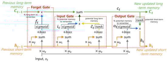
Figure 1.
The basic structure of a single LSTM unit.
In Figure 1, the green line that runs across the top of the unit is called the cell state and represents long-term memory. Although long-term memory can be modified by this multiplication and later by this addition, it should be noticed that there are no weights or biases that can alter it directly. The orange line is called the hidden state and represents short-term memories. Short-term memories are directly connected to consequences that can modify them. The forget gate stage in this LSTM unit determines what percentage of the long-term memory is remembered. The forget gate, , can be expressed as follows:
where is the weight matrix, is the bias, and is the sigmoid function.
The input gate has two blocks with blue and yellow lines. The block with the yellow line combines the short-term memory and the input to create a potential long-term memory. The block with the blue line determines what percentage of that potential memory to add to the long-term memory. The percentage and potential long-term memory (i.e., and ) can be calculated using Equations (2) and (3), respectively. The current updated long-term memory can be obtained using Equation (4).
where and are the weight matrixes, and and are the biases for each memory function.
With the updated long-term memory through the input gate, the final stage in this LSTM can be updated. The final stage updates the short-term memory. It can start with the updated long-term memory and use it as input to the tanh activation function. After the tanh activation function, the LSTM unit determines how much of the potential short-term memory to pass on. It thus creates the new short-term memory by multiplying the possible short-term memory and the percentage of potential long-term memory. Because of the recently updated short-term memory from this entire LSTM unit, this stage is called the output gate. The output gate can be calculated using Equation (5), and the recently updated short-term memory can be obtained using Equation (6).
where is the weight matrix, and is the bias. Among the hidden and cell states in the three gates, and represent the output of the currently updated and previous short-term memories, respectively. and represent the current and previously updated long-term memories. is the input variable in the LSTM unit. LSTM networks can avoid the exploding vanishing gradient problem by using separate paths for long-term and short-term memories. In addition, with the help of the three gates, an LSTM unit can read, reset, and update short- and long-term information for better performance of sequence prediction.
The concept of transfer learning (TL) involves a learning mechanism that reuses the weights obtained from related tasks in the past to solve new target tasks. TL mainly includes two domains: (1) a source domain and (2) a target domain. A source domain can be expressed as , and a target domain task can be expressed as . Domains consist of the feature space (i.e., ) and the marginal probability of the feature space (i.e., ). Among them, the feature space can be expressed as . Given the source and target domains (i.e., ), the domains’ tasks consist of the label space (i.e., ) and its conditional probability (i.e., ), which can be expressed as . is the learned knowledge from a source task (i.e., ), and it can be transferred to help solve new tasks (i.e., ) in a target domain. With the transfer learning method, fine tuning is the most effective transfer learning technique to update the weights of domain tasks already solved in the past and later migrate a portion of the weights to new tasks in a target domain. In the neural network layers, frozen and fine-tuning parts are described in detail in the later section. The backpropagation method is used when the fine-turned part is updated.
2.2. Description of the Building Model
This study used the prototype hospital building model [39] in the whole-building energy modeling software program, EnergyPlus [40], developed by the US Department of Energy (DOE) to create input and test datasets for LSTM-TL implementation. The prototype model complies with the minimum energy code requirements prescribed in ASHRAE Standard 90.1-2019 [41]. Figure 2 shows a three-dimensional perspective view of the prototype hospital model. The building model is configured as a five-story building with a rectangular floor plan, as shown in Figure 2. The construction of this building consists of a concrete block wall, wall insulation, and a gypsum board. Table 1 summarizes hospital building model characteristics. All input values and schedules regarding internal heat gains were directly obtained from the original version of a prototype hospital building model without modifications. The zone thermostat setpoint is set to 24 °C and 21 °C for cooling and heating, respectively. There is no thermostat setback operation during nighttime because many spaces are mostly occupied except for some office zones. Based on the outputs (e.g., lighting and plug-load electricity consumption) from this simulation model, the input dataset of LSTM-TL in a source domain was determined.
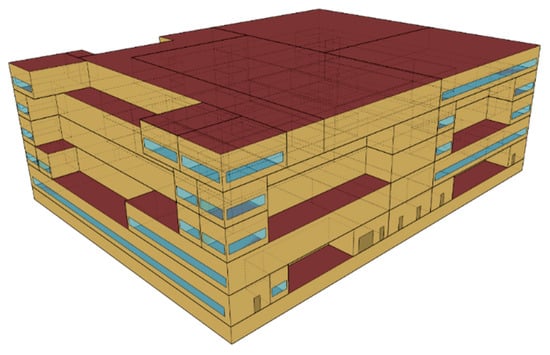
Figure 2.
Prototype hospital building model [39].

Table 1.
Prototype hospital building model characteristics.
The prototype hospital building model has VAV-type HVAC systems with natural gas boilers and chillers for thermal zones mostly. This VAV system is an air conditioning system that varies the supply air volume flow rate through the air handling units (AHUs) using dampers located in the VAV thermal box to curtail heating and cooling loads and meet the setpoint temperature. Figure 3 depicts HVAC zoning and its system types in the hospital building model. Except for the kitchen zone, all thermal zones use VAV-type systems. VAV 1 and 2 consist of typical AHUs with VAV reheat boxes. Humidifiers, extra water, and electric heating coils were added to the AHUs of other VAV systems (i.e., VAV ER, OR, ICU, Patient Room, and Laboratory). All the heating and cooling energy end-usages by gas boilers and chillers were considered for the training and testing datasets of the LSTM-TL predictions.
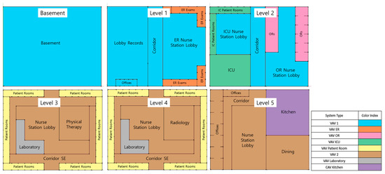
Figure 3.
HVAC zoning and system types [42].
2.3. Initial Source Data and Pre-Processing with Clustering Analysis
Because buildings can involve many associated energy factors, it is challenging to capture the information hidden under numerical data directly [43]. Thus, before conducting cluster analysis, we needed to ensure which subentry energy consumption was valuable to be analyzed. To carry out this purpose, the time series data associated with building energy consumption was investigated. Figure 4 presents the normalized data patterns of each energy-related value. Fifteen different types of data obtained from the simulation of the prototype hospital model are shown in this figure.
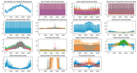
Figure 4.
Normalized raw data of the prototype hospital model.
Based on the data patterns above, cluster analysis was conducted via the following steps:
- Define an appropriate dataset format for time series data.
- Conduct scale standardization.
- Calculate appropriate inertia numbers.
- Conduct clustering analysis using the K-mean algorithm.
The cluster analysis was carried out as follows. Each time series dataset was considered in the first step. For example, the datasets from the EnergyPlus simulation were formed as , and the length of each data was based on the length of cooling and heating periods. N indicated the number of output variables. The initial numbers were output sets of 351 columns, but similar output types were grouped and shortened based on similar schedules and thermal zone conditions. Data standardization was carried out using Python language’s mean removal and variance scaling. Figure 5 presents the appropriate inertia number option. Four was considered the optimal K value for this study by considering the available measurement conditions and decreased inertia points. Based on the defined K number, the centroid was determined at random. The elements to the corresponding type are then described based on the distance between elements and the centroid. Finally, the centroid was recalculated according to the new aspects using expectation maximization and EM algorithms. The steps were iterated until the data converges with the defined value.
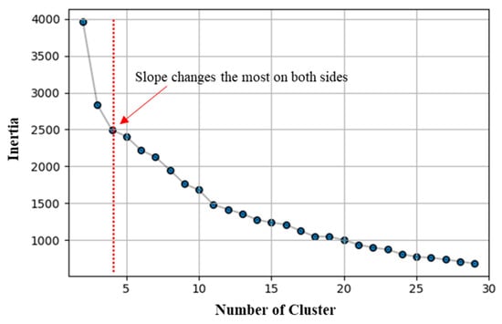
Figure 5.
Inertia results and selected K value calculated by the elbow method.
Based on the K value, this study conducted a pattern analysis to determine appropriate input variables for the energy consumption output layer, as shown in Figure 6. There were four distinguished patterns with normalized values. Based on this figure, it can be recognized that Cluster 1 indicates the internal heat gain patterns that have regular daily and weekly energy patterns. Cluster 2 shows relatively constant patterns except for during the middle of the summer period. The continual operation schedules (e.g., always on) are one of the factors that make these patterns relatively constant. In addition, the patterns of Cluster 3 and Cluster 4 seem to be heating- and cooling-related energy end-use. As described earlier, the major HVAC systems are VAV-type with chillers and boilers. However, some specific thermal zones include extra heating coils, air-to-air energy recovery units, and consistent operation schedules. Based on such patterns, this study distinguished the simulated data with similar patterns and grouped them for the data-driven model’s architecture and input/output layers.
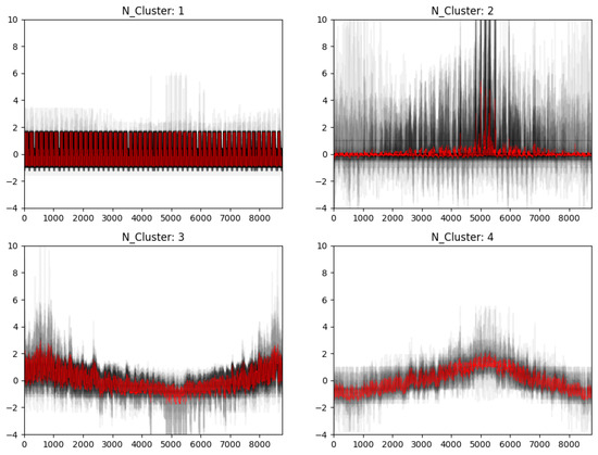
Figure 6.
Grouped patterns of clustering analysis.
Because cooling- and heating-related patterns highly depend on the outdoor conditions (e.g., outdoor air temperature and solar radiation), this study considered outdoor air temperature, humidity, and horizontal solar irradiation values as input variables. In addition, internal heat gain patterns (e.g., lighting and plug electricity usages) were also considered as input variables in the initial LSTM model.
2.4. Development of LSTM-TL Model
It is challenging to establish a high-accuracy forecasting model without sufficient data, especially with data-driven models. This study assumed that the target building has few current energy consumption data, making it difficult to train a load forecasting model independently and accurately. In addition, if there is a strong similarity between the simulated source buildings and the target buildings, the data that can be used for the target building prediction is relatively sufficient. With such assumptions, the simulated information was considered to build the input and output datasets in a source domain.
This section presents how this study developed the LSTM model and applied it to the transfer learning method. A data-driven model for building energy forecasting requires an input dataset with various variables, such as non-stationary outdoor weather conditions and relatively constant input patterns (e.g., scheduled lighting and base plug-loads). Although many factors affect building energy end-use, three main categories of input datasets, based on the cluster analysis in Section 2.3, can be considered for the building energy prediction, including (1) environmental, (2) historical, and (3) time-related data variables. Environmental data commonly depends on outdoor weather data, such as outdoor air temperature, relative humidity, and outside solar radiation. Historical data refers to past data measured and/or simulated that affects current indoor thermal behaviors due to some internal heat gain factors, such as occupant behaviors. This study did not consider occupant behaviors but reflected used internal heat gain demands (e.g., lighting and plug loads) based on scheduled occupant behaviors in a simulation environment. Time-related information refers to the data length, time, and seasons, which can be expressed in hours or months. Time-related data is also important because it can reflect the HVAC operation time during daytime and nighttime and operation seasons (e.g., cooling and heating).
Figure 7 shows the architecture of the number of input, hidden, and output layers and each node of the model. The number of layers and nodes was directly obtained from Ahn’s study [36], but the input parameters were modified based on the current clustering analysis. The architecture used for this study included five LSTM layers with 8, 16, 32, 32, and 64 nodes. The final dense layer was then one node. The input variables were set to the outside temperature, relative humidity, solar irradiation, month, time, scheduled internal heat gains, and temperature differences between outdoor and indoor air temperatures.
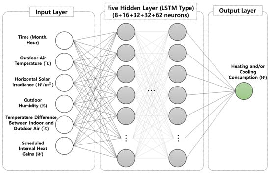
Figure 7.
Input, hidden, and output layers architecture used for LSTM.
This study used scikit-learn and Keras in Python to implement the stacked LSTM. With the scikit-learn and Keras modules in Python, Numpy, pandas, and matplotlib modules were also used to process the time series data organization, data frame, and visualization. The major parameters for the establishment of the initial stacked LSTM prediction models were set as follows (1) Learning rate: 0.001, (2) Batch size: 10, (3) Sequence length: 3, (4) Training rate: 0.8, (5) Epochs: 100, and (6) Dropout: 0.5. Based on a similar study in the literature review [35,36], these hyper-parameters were empirically determined to obtain a suitable combination that could result in higher performance.
This study used the Adam optimization function with a learning rate value of 0.001 and the Sigmoid activation function. Based on the literature [32,35,36], a dropout rate of 0.5 was used to prevent overfitting, and the dropout could only be applied to the LSTM 5 layers. The LSTM model was trained for 100 epochs with ten as the batch size. In addition, MinMaxScaler was used to reflect that pre-processing and post-processing were performed to unify the energy units of the output. The training and test datasets were divided into 80% and 20% for training and test datasets, respectively.
For the source domain, the model was trained using four months of simulated data from the source datasets and verified against one month of the datasets. Transfer learning (TL) was used for the target domain to combine the target dataset with the learned knowledge obtained from the source domain. Figure 8 represents the workflow of LSTM with a transfer learning application used for this study. Each target data of cooling and heating was also trained and tested using the LSTM models for comparison before and after the transfer learning application.
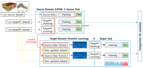
Figure 8.
Workflow of LSTM with a transfer learning method.
Regarding the TL process, the three different layers applied in this study were frozen, fine-turning, and partially frozen to reuse the weights for comparative analysis. Figure 9 depicts the LSTM-TL options for the comparative analysis. The frozen layer option can be considered as the same LSTM model because the all-frozen layer indicates that the trainable parameters are zero, which means the fine tuning does not occur during the TL process. These options can be further used for comparative analysis with the LSTM model.
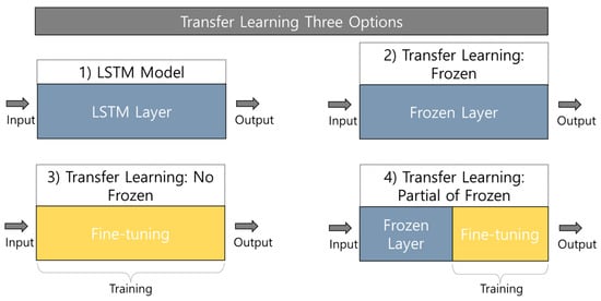
Figure 9.
LSTM-TL options for comparative analysis.
2.5. The Location Selection of Target Tasks
The hospital prototype building models were placed in four cities in South Korea to generate testing data for target domain tasks. This study considered the four weather data locations that the EnergyPlus weather data website officially provides [44]. The EnergyPlus website provides typical meteorological year version 3 (TMY3) for hourly weather files of the city, which is based on design conditions from the climate design data ASHRAE Handbook [45], to calculate heating and cooling loads [45]. Figure 10 and Figure 11 show the compared values of each city’s weather data for cooling and heating periods, respectively, including global horizontal irradiance (GHI) with units, W/m², outdoor air-dry bulb temperature, and relative humidity. The cooling period graph was created based on the weather data values for August, while the heating period used for this weather graph was January. The box and whisker diagram of each comparison indicates the maximum, minimum, mean, and other values, as shown in the figures. The three values (i.e., GHI, OA temperature, and relative humidity) were directly used for the input dataset of the developed LSTM model. Daejeon was used for source domain tasks, and other locations were thus used for target domain tasks in this study.
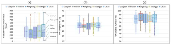
Figure 10.
Weather data comparison of representative cities for cooling period (August): (a) global horizontal irradiance, (b) outdoor air-dry bulb temperature, and (c) outdoor air relative humidity values.
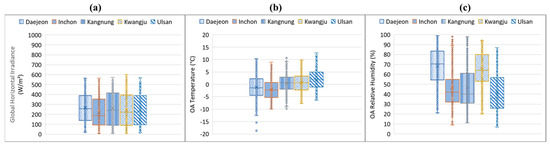
Figure 11.
Weather data comparison of representative cities for heating period (January): (a) global horizontal irradiance, (b) outdoor air-dry bulb temperature, and (c) outdoor air relative humidity values.
Figure 12 presents an example of the raw input dataset used for target domain tasks in the Inchone location. Six variables, including time data (i.e., month and hour), were used as input datasets, and the one output was the hourly building energy end-use value, as mentioned earlier. As seen in this figure, the internal heat gain energy use, such as plug load and lighting, shows regularly similar patterns throughout the period. In contrast, other input variables (e.g., temperature difference and energy end-use) present significantly different patterns depending on outdoor weather conditions. The building energy end-use data was used for the prediction output, and the test period is shown within a rectangular dot box, which was determined based on the training rate, 0.8. The target domain tasks were performed using LSTM TL analysis based on such datasets.
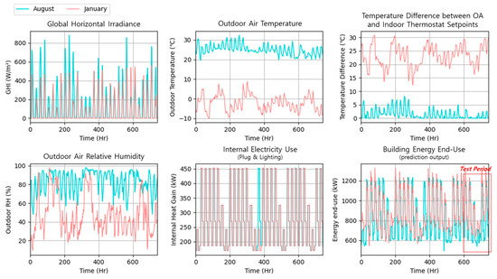
Figure 12.
An example of the raw input dataset used for a target domain task of TL analysis for the simulated prototype hospital model in the Inchon location.
2.6. Performance Metrics for Validation and Testing Models
For statistical evaluation, this study used three criteria—the coefficient of variation of the root means squared error (CVRMSE), normalized mean bias error (NMBE), and the coefficient of determination ()—to validate the developed LSTM-TL models and determine how well they fit with the measured data based on ASHRAE Guideline 14 [46]. The calculation equations are as follows:
where is the measured data sample, is the predicted data sample, is mean values, and is the number of data samples, with . is a measure of the extent to which the regression model explains variations in the dependent variable from its mean value [46]. Based on three criteria, the LSTM-LT models were tested and validated for this study.
3. Results and Discussion
This section presents the results and discussion obtained from the cooling and heating predictions using the LSTM model with a transfer learning method. For the data used as a source domain, the simulated data of the prototype hospital building model was used. The simulated data in other locations were then used to implement the LSTM-transfer learning (TL) model for the cooling and heating predictions in the target domain. The first part of this section compares energy consumption predictions of source domain tasks for cooling and heating periods using the initial LSTM model. Target domain tasks with LSTM-TL options are then compared to investigate how the TL techniques can change the performance accuracy of building energy consumption for cooling and heating periods with different location data sources.
3.1. Comparison of Source Data Predictions without Transfer Learning for the Cooling and Heating Periods
Figure 13 and Figure 14 show a comparison of the hospital building’s energy consumption for the representative cooling and heating periods using the 5-month simulated data. The 5-month simulated data was first used for training and testing using the initially developed LSTM model for each season. This study assumes that the cooling period is from May to September, and the heating period is from November to March. During the cooling period, the building energy end-use used for this analysis did not include heating-related energy consumption, such as natural gas usage consumed by heating boilers. Therefore, the building energy consumption for this period indicates the internal heat gain-related electricity use (e.g., lighting and plug demands) and cooling-related electricity use (e.g., chillers, AHU fans, and extra electrical reheat coils). In contrast, for the heating period, the main heating coils in AHUs associated with heating boilers and extra electrical reheat coils are the main energy parts in the building’s energy consumption instead of the cooling-related components. The internal heat gain-related electricity end-use is also one of the contributors to building energy consumption with the heating-related energy components.
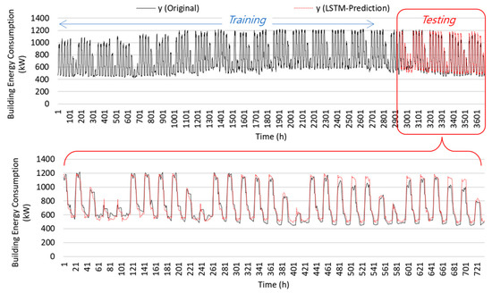
Figure 13.
Comparison of source data prediction without transfer learning for the cooling period.
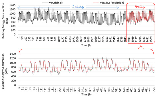
Figure 14.
Comparison of source data prediction without transfer learning for the heating period.
With the simulated data, the LSTM model was trained using 80% of the data and results in 20% of the test results. About four and a half weeks were considered for the testing period. Figure 13 shows the compared patterns of the hospital building’s energy prediction with the simulated data. Because the building type is a hospital, many baseloads are always on in operation during daytime and nighttime for occupants (e.g., patients). Overall, the compared results show that the initially developed LSTM model has an acceptable prediction accuracy with good agreements with the CV(RMSE) value of 24.96 % and value of 0.90. Examining Figure 13’s pattern comparison, the LSTM model shows good energy load forecasting results in the first and second weeks. On the contrary, some overpredicted patterns were observed during the daytime and nighttime two and half weeks into the testing period. The overpredictions tended to occur at the middle and end of September, during relatively cool and low-humidity outdoor air conditions compared to the training period. Although the internal heat gain-related energy end-use has similar patterns throughout all seasons, cooling-related energy components highly depend on non-stationary outdoor weather conditions. Each month used for the training and testing data had different outdoor conditions and patterns, even if they are in the cooling-dominant period, which could reduce the performance accuracy of predicted values. For example, the energy end-use for air-to-air energy recovery units and some cooling coils tend to be less during that period with such mild weather conditions.
Figure 14 compares building energy predictions for the heating period when the LSTM model used the 5-month simulated data. The same training and testing periods were also used for the LSTM heating prediction. As expected, using simulated data with sufficient data lengths can show good performance of the time series forecasting. The overall comparison patterns present good prediction accuracy for the heating period in the source domain task, with a CV(RMSE) value of 16.62% and an value of 0.89. CV(RMSE) values of less than 30% indicate acceptable prediction performance with an hourly database. Because this study assumes that the heating period is between November and March, the testing period of the heating domain task was mostly in March, during which the weather conditions were relatively mild. Compared to the cooling period’s CV(RMSE) value, the heating period comparison shows relatively high prediction accuracy. Except for some weekends, the prediction patterns show good fits against the original simulation data. During weekends of the heating period, overpredicted points usually occurred because this study did not consider separate indexing for weekdays and weekends, which can lead to less accurate predictions.
Table 2 shows the overall statistical results, which include the number of accurate prediction performances with differently compared seasons. As expected, examining this table, the simulated data-based training and testing cases present acceptable prediction accuracy in the cooling and heating comparison. The estimated values were 0.90 and 0.89 for cooling and heating periods, respectively. Table 2 also shows the CV(RMSE) values for each period. Although the CV(RMSE) value of the heating period was higher than the cooling period value, the comprehensive CV(RMSE) values of both periods were acceptable for building energy prediction. This trend indicates that predicted outputs can be expected to demonstrate good accuracy when sufficient datasets are used for the data-driven model. Based on such results, this study considered a transfer learning technique, assuming that limited input datasets are only available for target domain tasks. The next two sections compare target data predictions with transfer learning options for the cooling and heating periods.
Table 2.
Statistical results of LSTM prediction performance.
3.2. Comparison of Target Data Predictions with Transfer Learning Options for the Cooling Period
This section presents transfer learning (TL)-based analysis for the cooling and heating periods. As can be seen in Figure 8, there were the source and target domains. For the source domain, the basic LSTM models for each season were initially developed with the source domain dataset. Based on the developed LSTM models, the target domain datasets were reflected for TL’s potential in the different locations, presented in Section 2.5. Three other TL options were considered for this comparative analysis, including all frozen layers, fine-tuning layers, and partially frozen layers, as shown in Figure 9. In the graph, the frozen layer option is expressed as “y(LSTM-Option 2)” because the presence of all frozen layers indicates that the trainable parameters are zero. The “y(LSTM-TL Option 3)” is the fine-tuning option, which suggests that all the trainable params are considered for the fine tuning of the prediction model. The partially frozen layer is expressed as “y(LSTM-TL Option 4)” in graphs. For this option, three layers are considered for fine tuning, and other layers are frozen when the machine updates the prediction model.
Figure 15 shows the prediction comparison of the target data with TL options for each selected location. As mentioned earlier, a 1-month dataset from August was used in this target domain task. Similar to the source task, 80% and 20% of the same dataset lengths were considered for training and testing, respectively. A comparison of testing results using the target data is shown in Figure 15 for about six days (i.e., 20% of the test dataset).
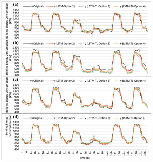
Figure 15.
Comparison of the target prediction with transfer learning options for the cooling period: (a) Inchon, (b) Kangnung, (c) Kwangju, and (d) Ulsan cities.
Overall, the prediction accuracy of building energy end-use prediction can be improved by implementing the TL process for the compared cooling period in all locations. As seen in this figure, it can be observed that the developed LSTM-TL model significantly improves the accuracy of the building energy prediction compared to the LSTM model with a newly given target task based on the limited datasets. For example, examining Figure 14a, the hourly prediction patterns of the LSTM-TL models show closer matches in most hours to the originally simulated data compared to the only LSTM-used prediction (i.e., LSTM-Option 2). In addition, high improvement patterns can be typically observed during the afternoon on weekdays in most locations when the full and partial fine-tuning processes are reflected.
Table 3 summarizes the statistical results for each prediction scenario of each city. Examining this table, although the LSTM predictions of all locations show acceptable results, the TL process can make more prediction improvements with the relatively sufficient source datasets but limited target datasets that this study assumed. For example, the Ulsan location showed a 22.5% CV(RMSE) value for LSTM-Option 2. However, when the TL process was considered, the prediction accuracy improved, producing CV(RMSE) values of 17.3% and 15.3% for TL-Option 3 and TL-Option 4, respectively. In addition, the estimated values improved using the TL options in most locations. An value of 0.9 was captured for LSTM-Option 2, and its value was then improved to 0.95 for both TL options. For the cooling period, TL-Option 4, which was based on the partial fine-tuning strategy, showed better improvement for all locations than TL-Option 3.
Table 3.
Statistical results of LSTM prediction performance with transfer learning for the cooling period.
3.3. Comparison of Target Data Predictions with Transfer Learning Options for the Heating Period
Figure 16 compares the predicted energy end-use results for the target domain tasks during heating when the TL process was adopted with limited target data in different locations. The prototype hospital building was simulated using four other locations to generate a 1-month dataset in January. As mentioned earlier, this heating energy analysis used the same training rate.
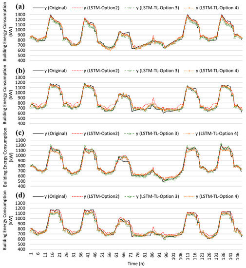
Figure 16.
Comparison of the target prediction with transfer learning options for the heating period: (a) Inchon, (b) Kangnung, (c) Kwangju, and (d) Ulsan cities.
The compared patterns of prediction results are shown in Figure 16a–d for Inchon, Kangnung, Kwangju, and Ulsan locations, respectively. As expected, this study identifies that with the help of the TL process, the prediction accuracy of the LSTM-TL model can be improved for heating energy end-use in all locations. For example, in the Kangnung location, LSTM-Option 2 model mostly underpredicted the energy end-use during nighttime. However, when the TL process was used for the target tasks, the hourly prediction patterns of the LSTM-TL models (i.e., LSTM-Option 3 and 4) presented closer matches in most time steps to the original baseline data. For Kwangju, different patterns of prediction improvement were captured compared to the Kangnung location. The LSTM-Option 2 model presented some overpredicted patterns during the daytime for the first three days, but the prediction became gradually more accurate with the TL process. In addition, some spike data patterns can be flattened to match the patterns closer to the baseline during weekends with the help of the TL strategy, which improved overall prediction accuracy in most locations.
Table 4 summarizes the statistical results of prediction performance with TL options for the heating period. All locations show acceptable prediction accuracy with good agreements for LSTM-Option 2, producing CV(RMSE) values of 11.54%, 20.2%, 13.86%, and 13.97% for Inchon, Kangnung, Kwangju, and Ulsan, respectively. The predicted values for LSTM-Option 2 also achieve good results, presenting values of 0.955, 0.896, 0.946, and 0.932 for Inchon, Kangnung, Kwangju, and Ulsan, respectively. Prediction performance can thus be improved when the full fine-tuning and partial fine-tuning strategies are reflected for the prediction. The improvement rate can vary according to the location. For example, the CV(RMSE) values were 11.05% and 11.13% for LSTM-Options 3 and 4, respectively, in Kangnung, which were about 45% higher compared to LSTM-Option 2. For the Inchon location, even though the performance accuracy tended to improve with the help of TL strategies, the increased CV(RMSE) values shown were lower than in other locations. However, based on the observed results, this study identifies that the TL strategies achieved improved prediction performance for all sites with the 1-month datasets from the only LSTM-used prediction.
Table 4.
Statistical results of LSTM prediction performance with transfer learning for the heating period.
4. Conclusions
To effectively solve the prediction problem of the time series prediction model under a practically insufficient dataset, this paper presented the implementation of a data-driven model with a transfer learning method. The prototype hospital building type model was used to create sequential input and output datasets in source and target domains for the data-driven model. Two simulation periods were considered to separate cooling and heating predictions under the simulated analysis environment: (1) the cooling period was between May and September, and (2) the heating period was between November and March. The basic LSTM models were initially developed using the simulated cooling and heating datasets for a source domain task. After the development of the LSTM model, the shortened simulation data for cooling and heating periods was also used with transfer learning in the target domain to effectively overcome the prediction problem with practically insufficient datasets in different weather conditions. Based on full and partial fine-tuning techniques of a transfer learning method, a basic LSTM model was improved for better prediction accuracy.
The results showed that, with the help of transfer learning technology, the LSTM model improved hourly building energy use prediction accuracy with relatively limited datasets. When the LSTM model used sufficient simulation datasets, the prediction model showed good accuracy in the sequence energy forecasting, as expected, for source tasks. With 1-month of simulated datasets, the predictions of the LSTM model also presented acceptable prediction accuracy by showing close matches in most compared time steps. When TL strategies were reflected in the prediction process for target domain tasks, the prediction accuracy was significantly improved with a better coefficient of determination and better CV(RMSE) values. Although the improvement range can vary according to different weather conditions, all locations selected in this paper experienced improved prediction accuracy with the help of TL strategies. It should be noted that because this analysis was based on simulation-based analysis to set up input parameters and their datasets, the improvement could be significant without practically occurring uncertainties. Furthermore, if actual field measurements were considered for target domain tasks, the improved ranges of prediction accuracy could be varied according to the analysis conditions.
Even though the transfer learning model can markedly improve the accuracy of the prediction model with relatively small datasets, there are still concerns about practical applications considering various building types and weather conditions. In addition, such prediction work based on data-driven methods is still a beginning step toward solving the complicated building load forecasting problem with insufficient data. Although this study conducted clustering analysis to capture major input variables for the prediction model, it has some limited assumptions, such as the details of the separate week and weekend days, occupant behaviors, and hyper-parameter optimization. Based on the current research, the detailed analysis of energy simulation and measurement methods for various building types and conditions for time series data is another research topic based on optimized input parameters in the future to further improve prediction accuracy under non-stationary conditions.
Author Contributions
Conceptualization, D.K., Y.L. and H.C.; methodology, D.K., K.C., Y.L. and H.C.; formal analysis, D.K., H.C. and J.Z.; investigation, D.K., Y.L. and H.C.; data curation, D.K. and H.C.; writing—original draft preparation, D.K., H.C., P.J.M. and J.Z.; writing—review and editing, D.K., K.C., Y.L., P.J.M., J.Z. and H.C.; visualization, D.K. and H.C.; supervision, D.K., Y.L. and H.C.; funding acquisition, D.K. and Y.L. All authors have read and agreed to the published version of the manuscript.
Funding
This work was supported by the Korea Agency for Infrastructure Technology Advancement (KAIA) grant funded by the Ministry of Land, Infrastructure and Transport (Grant RS-2019-KA153277).
Institutional Review Board Statement
Not applicable.
Informed Consent Statement
Not applicable.
Data Availability Statement
Not applicable.
Conflicts of Interest
The authors declare no conflict of interest.
Nomenclature
| AHU | air-handling unit |
| AI | artificial intelligence |
| AM | attention mechanism |
| ANN | artificial neural networks |
| ARIMA | autoregressive integrated moving averages |
| ARX | exogenous inputs |
| ASHRAE | the American Society of Heating, Refrigerating, and Air-Conditioning Engineers |
| CNN | convolutional neural networks |
| CV(RMSE) | the coefficient of variation of the root means squared error |
| DOE | department of energy |
| DWT | discrete wavelet transform |
| EIA | energy information administration |
| GHG | greenhouse gas |
| HVAC | cooling, heating, and air-conditioning |
| LSTM | long short-term memory |
| ML | machine learning |
| MLR | multiple linear regression |
| NMBE | normalized mean bias error |
| RNN | recurrent neural networks |
| TL | transfer learning |
| VAV | variable air volume |
References
- U.S. EIA. Global Energy & CO2 Status Report: The Latest Trends in Energy and Emissions in 2018; U.S. EIA: Washington, DC, USA, 2018.
- U.S. EIA. EIA: International Energy Outlook 2019 with Projections to 2050; U.S. EIA: Washington, DC, USA, 2019.
- Zhao, H.X.; Magoulès, F. A Review on the Prediction of Building Energy Consumption. Renew. Sustain. Energy Rev. 2012, 16, 3586–3592. [Google Scholar] [CrossRef]
- Lawrence, T.; Abdel, K.; Darwich, J.K.M. ASHRAE GreenGuide: Design, Construction and Operation of Sustainable Buildings; ASHRAE: Peachtree Corners, GA, USA, 2018; ISBN 9781939200808. [Google Scholar]
- Kim, D.; Yoon, Y.; Lee, J.; Mago, P.J.; Lee, K.; Cho, H. Design and Implementation of Smart Buildings: A Review of Current Research Trend. Energies 2022, 15, 4278. [Google Scholar] [CrossRef]
- Kim, D.; Cox, S.J.; Cho, H.; Yoon, J. Comparative Investigation on Building Energy Performance of Double Skin Façade (DSF) with Interior or Exterior Slat Blinds. J. Build. Eng. 2018, 20, 411–423. [Google Scholar] [CrossRef]
- Kim, D.; Cox, S.J.; Cho, H.; Im, P. Evaluation of Energy Savings Potential of Variable Refrigerant Flow (VRF) from Variable Air Volume (VAV) in the U.S. Climate Locations. Energy Rep. 2017, 3, 85–93. [Google Scholar] [CrossRef]
- Hong, T.; Chou, S.; Bong, T. Building Simulation: An Overview of Developments and Information Sources. Build. Environ. 2000, 35, 347–361. [Google Scholar] [CrossRef]
- Afroz, Z.; Shafiullah, G.M.; Urmee, T.; Higgins, G. Modeling Techniques Used in Building HVAC Control Systems: A Review. Renew. Sustain. Energy Rev. 2018, 83, 64–84. [Google Scholar] [CrossRef]
- Wang, Z.; Hong, T. Reinforcement Learning for Building Controls: The Opportunities and Challenges. Appl. Energy 2020, 269, 115036. [Google Scholar] [CrossRef]
- Hajjaji, Y.; Boulila, W.; Farah, I.R.; Romdhani, I.; Hussain, A. Big Data and IoT-Based Applications in Smart Environments: A Systematic Review. Comput. Sci. Rev. 2021, 39, 100318. [Google Scholar] [CrossRef]
- Norouziasl, S.; Jafari, A.; Zhu, Y. Modeling and Simulation of Energy-Related Human-Building Interaction: A Systematic Review. J. Build. Eng. 2021, 44, 102928. [Google Scholar] [CrossRef]
- Chen, Y.; Guo, M.; Chen, Z.; Chen, Z.; Ji, Y. Physical Energy and Data-Driven Models in Building Energy Prediction: A Review. Energy Rep. 2022, 8, 2656–2671. [Google Scholar] [CrossRef]
- Pedersen, L.; Stang, J.; Ulseth, R. Load Prediction Method for Heat and Electricity Demand in Buildings for the Purpose of Planning for Mixed Energy Distribution Systems. Energy Build. 2008, 40, 1124–1134. [Google Scholar] [CrossRef]
- Ahmad, T.; Chen, H.; Guo, Y.; Wang, J. A Comprehensive Overview on the Data Driven and Large Scale Based Approaches for Forecasting of Building Energy Demand: A Review. Energy Build. 2018, 165, 301–320. [Google Scholar] [CrossRef]
- Bourdeau, M.; Zhai, Q.X.; Nefzaoui, E.; Guo, X.; Chatellier, P. Modeling and Forecasting Building Energy Consumption: A Review of Data-Driven Techniques. Sustain. Cities Soc. 2019, 48, 101533. [Google Scholar] [CrossRef]
- Cox, S.J.; Kim, D.; Cho, H.; Mago, P. Real Time Optimal Control of District Cooling System with Thermal Energy Storage Using Neural Networks. Appl. Energy 2019, 238, 466–480. [Google Scholar] [CrossRef]
- Afram, A.; Janabi-Sharifi, F.; Fung, A.S.; Raahemifar, K. Artificial Neural Network (ANN) Based Model Predictive Control (MPC) and Optimization of HVAC Systems: A State of the Art Review and Case Study of a Residential HVAC System. Energy Build. 2017, 141, 96–113. [Google Scholar] [CrossRef]
- Yu, B.; Kim, D.; Cho, H.; Mago, P. A Nonlinear Autoregressive with Exogenous Inputs Artificial Neural Network Model for Building Thermal Load Prediction. J. Energy Resour. Technol. Trans. ASME 2020, 142, 050902. [Google Scholar] [CrossRef]
- Gao, Y.; Ruan, Y.; Fang, C.; Yin, S. Deep Learning and Transfer Learning Models of Energy Consumption Forecasting for a Building with Poor Information Data. Energy Build. 2020, 223, 110156. [Google Scholar] [CrossRef]
- Zhou, S.; Guo, S.; Du, B.; Huang, S.; Guo, J. A Hybrid Framework for Multivariate Time Series Forecasting of Daily Urban Water Demand Using Attention-Based Convolutional Neural Network and Long Short-Term Memory Network. Sustainability 2022, 14, 11086. [Google Scholar] [CrossRef]
- Ünlü, K.D. A Data-Driven Model to Forecast Multi-Step Ahead Time Series of Turkish Daily Electricity Load. Electronics 2022, 11, 1524. [Google Scholar] [CrossRef]
- Hajiabotorabi, Z.; Kazemi, A.; Samavati, F.F.; Maalek Ghaini, F.M. Improving DWT-RNN Model via B-Spline Wavelet Multiresolution to Forecast a High-Frequency Time Series. Expert Syst. Appl. 2019, 138, 112842. [Google Scholar] [CrossRef]
- Deb, C.; Schlueter, A. Review of Data-Driven Energy Modelling Techniques for Building Retrofit. Renew. Sustain. Energy Rev. 2021, 144, 110990. [Google Scholar] [CrossRef]
- Gers, F. Long Short-Term Memory in Recurrent Neural Networks. Ph.D. Thesis, École Polytechnique Fédérale de Lausanne (EPFL), Lausanne, Switzerland, 2001; p. 2366. [Google Scholar]
- Zhou, Y.; Wang, L.; Qian, J. Application of Combined Models Based on Empirical Mode Decomposition, Deep Learning, and Autoregressive Integrated Moving Average Model for Short-Term Heating Load Predictions. Sustainability 2022, 14, 7349. [Google Scholar] [CrossRef]
- Durand, D.; Aguilar, J.; R-Moreno, M.D. An Analysis of the Energy Consumption Forecasting Problem in Smart Buildings Using LSTM. Sustainability 2022, 14, 13358. [Google Scholar] [CrossRef]
- Cao, J.; Li, Z.; Li, J. Financial Time Series Forecasting Model Based on CEEMDAN and LSTM. Phys. A Stat. Mech. Its Appl. 2019, 519, 127–139. [Google Scholar] [CrossRef]
- Choi, E.; Cho, S.; Kim, D.K. Power Demand Forecasting Using Long Short-Term Memory (LSTM) Deep-Learning Model for Monitoring Energy Sustainability. Sustainability 2020, 12, 1109. [Google Scholar] [CrossRef]
- Li, G.; Zhao, X.; Fan, C.; Fang, X.; Li, F.; Wu, Y. Assessment of Long Short-Term Memory and Its Modifications for Enhanced Short-Term Building Energy Predictions. J. Build. Eng. 2021, 43, 103182. [Google Scholar] [CrossRef]
- Liu, J.; Ma, C.; Gui, H.; Wang, S. Transfer Learning-Based Thermal Error Prediction and Control with Deep Residual LSTM Network. Knowl.-Based Syst. 2022, 237, 107704. [Google Scholar] [CrossRef]
- Park, H.; Park, D.Y.; Noh, B.; Chang, S. Stacking Deep Transfer Learning for Short-Term Cross Building Energy Prediction with Different Seasonality and Occupant Schedule. Build. Environ. 2022, 218, 109060. [Google Scholar] [CrossRef]
- Peng, C.; Tao, Y.; Chen, Z.; Zhang, Y.; Sun, X. Multi-Source Transfer Learning Guided Ensemble LSTM for Building Multi-Load Forecasting. Expert Syst. Appl. 2022, 202, 117194. [Google Scholar] [CrossRef]
- Ma, J.; Cheng, J.C.P.; Jiang, F.; Chen, W.; Wang, M.; Zhai, C. A Bi-Directional Missing Data Imputation Scheme Based on LSTM and Transfer Learning for Building Energy Data. Energy Build. 2020, 216, 109941. [Google Scholar] [CrossRef]
- Li, G.; Wu, Y.; Liu, J.; Fang, X.; Wang, Z. Performance Evaluation of Short-Term Cross-Building Energy Predictions Using Deep Transfer Learning Strategies. Energy Build. 2022, 275, 112461. [Google Scholar] [CrossRef]
- Ahn, Y.; Kim, B.S. Prediction of Building Power Consumption Using Transfer Learning-Based Reference Building and Simulation Dataset. Energy Build. 2022, 258, 111717. [Google Scholar] [CrossRef]
- Mocanu, E.; Nguyen, P.H.; Kling, W.L.; Gibescu, M. Unsupervised Energy Prediction in a Smart Grid Context Using Reinforcement Cross-Building Transfer Learning. Energy Build. 2016, 116, 646–655. [Google Scholar] [CrossRef]
- Fang, X.; Gong, G.; Li, G.; Chun, L.; Li, W.; Peng, P. A Hybrid Deep Transfer Learning Strategy for Short Term Cross-Building Energy Prediction. Energy 2021, 215, 119208. [Google Scholar] [CrossRef]
- US DOE Building Energy Codes Program-Prototype Building Models. Available online: https://www.energycodes.gov/prototype-building-models (accessed on 16 June 2021).
- US DOE. EnergyPlus. Available online: https://energyplus.net (accessed on 30 September 2021).
- US DOE. Energy Savings Analysis: ANSI/ASHRAE/IES Standard 90.1-2019; US DOE: Washington, DC, USA, 2021.
- DOE Prototype Building Models-Building Energy Codes Program. Available online: https://www.energycodes.gov/prototype-building-models#Commercial (accessed on 3 January 2023).
- Liu, X.; Sun, H.; Han, S.; Han, S.; Niu, S.; Qin, W.; Sun, P.; Song, D. A Data Mining Research on Office Building Energy Pattern Based on Time-Series Energy Consumption Data. Energy Build. 2022, 259, 111888. [Google Scholar] [CrossRef]
- US DOE Weather Data by Country. Available online: https://energyplus.net/weather-region/asia_wmo_region_2/KOR (accessed on 16 June 2020).
- ASHRAE. ASHRAE Fundamentals (SI); ASHRAE: Peachtree Corners, GA, USA, 2017; ISBN 6785392187. [Google Scholar]
- ASHRAE. Guideline 14-2014 Measurement of Energy, Demand, and Water Savings; ASHRAE: Peachtree Corners, GA, USA, 2014; Volume 4, pp. 1–150. [Google Scholar]


Disclaimer/Publisher’s Note: The statements, opinions and data contained in all publications are solely those of the individual author(s) and contributor(s) and not of MDPI and/or the editor(s). MDPI and/or the editor(s) disclaim responsibility for any injury to people or property resulting from any ideas, methods, instructions or products referred to in the content. |
© 2023 by the authors. Licensee MDPI, Basel, Switzerland. This article is an open access article distributed under the terms and conditions of the Creative Commons Attribution (CC BY) license (https://creativecommons.org/licenses/by/4.0/).