A Contamination Predictive Model for Escherichia coli in Rural Communities Dug Shallow Wells

Abstract

In Brazilian rural communities, the lack of treated water leads their residents to seek individual and alternative solutions, in which dug shallow wells (DSW) are quite widespread. However, water quality may not be fitted for human consumption. For this reason, the current study aimed to predict the contamination of DSW water in rural communities in the Brazilian state of Goiás. For this, secondary data related to water quality, the distance to possible contamination sources, structural conditions, and local geology were evaluated. Therefore, a generalized linear model was applied, and its predictors were evaluated by stepwise methods (Akaike information criterion—AIC and Bayesian information criterion—BIC), generating an intermediate model. After the analysis, turbidity parameter was chosen to be removed resulting in a final, submitted to leave-one-out cross-validation method, and its performance was measured by a confusion matrix. The final model resulted in four predictive variables: well diameter, contour paving width, poultry, and swine husbandry existence. The model accuracy was 82.61%, with a true positive predictor of 82.18% and a negative predictor of 85.71%.

1. Introduction

In rural communities, using alternative water supply sources is common. Among these are dug shallow wells (DSW) or simply excavated wells locally known as cacimba, cacimbão, poço raso, poço Amazonas, cisterna, among others [1]. However, elsewhere in the world, other terms are used, such as dug wells [2], shallow wells [3], and hand-dug wells [4].

These water sources use groundwater, and its contamination due microorganisms is frequently reported in the literature, reporting the presence of rudimentary cesspools [2,3,4], pigsties [5,6,7], corrals [8,9,10], poultry [11], among others [12,13].

Contaminated water consumption can cause a series of waterborne diseases, mainly infections related to pathogenic organisms’ presence in humans and animals [14,15,16]. Identifying these microorganisms and the inactivate pathogens present in water is the subject of several studies [17,18,19]. However, verifying the level of contamination is usually done through physical-chemical and microbiological analyses [20,21], demanding high costs and time to obtain adequate information. Therefore, predicting the contamination of a given water source can often be less expensive and offer better efficiency [22,23,24].

However, it is necessary to select possible contamination sources and their characteristics, related to water quality. In this context, predictors associated with land use, population density, livestock and poultry densities, sanitary condition, antecedent precipitation, groundwater quality, aquifer characteristics, and groundwater hydrology are generally used [25].

For water contamination prediction, generalized linear models (GLM) can be applied, in which the coefficients related to each predictor provide a probability forecast, allowing parametric and non-parametric models to use. However, the research deficit of contamination prediction by GLM in DSW waters is notorious, in which few studies related to this subject use a binomial model, through grouped binary data (yes or no), being adequate to apply logistic regression [26,27].

Thus, the present study aimed to adjust a GLM, capable of predicting the probability of contamination by Escherichia coli in DSW located in rural communities in the State of Goiás, as a function of predictive environmental variables.

2. Materials and Methods

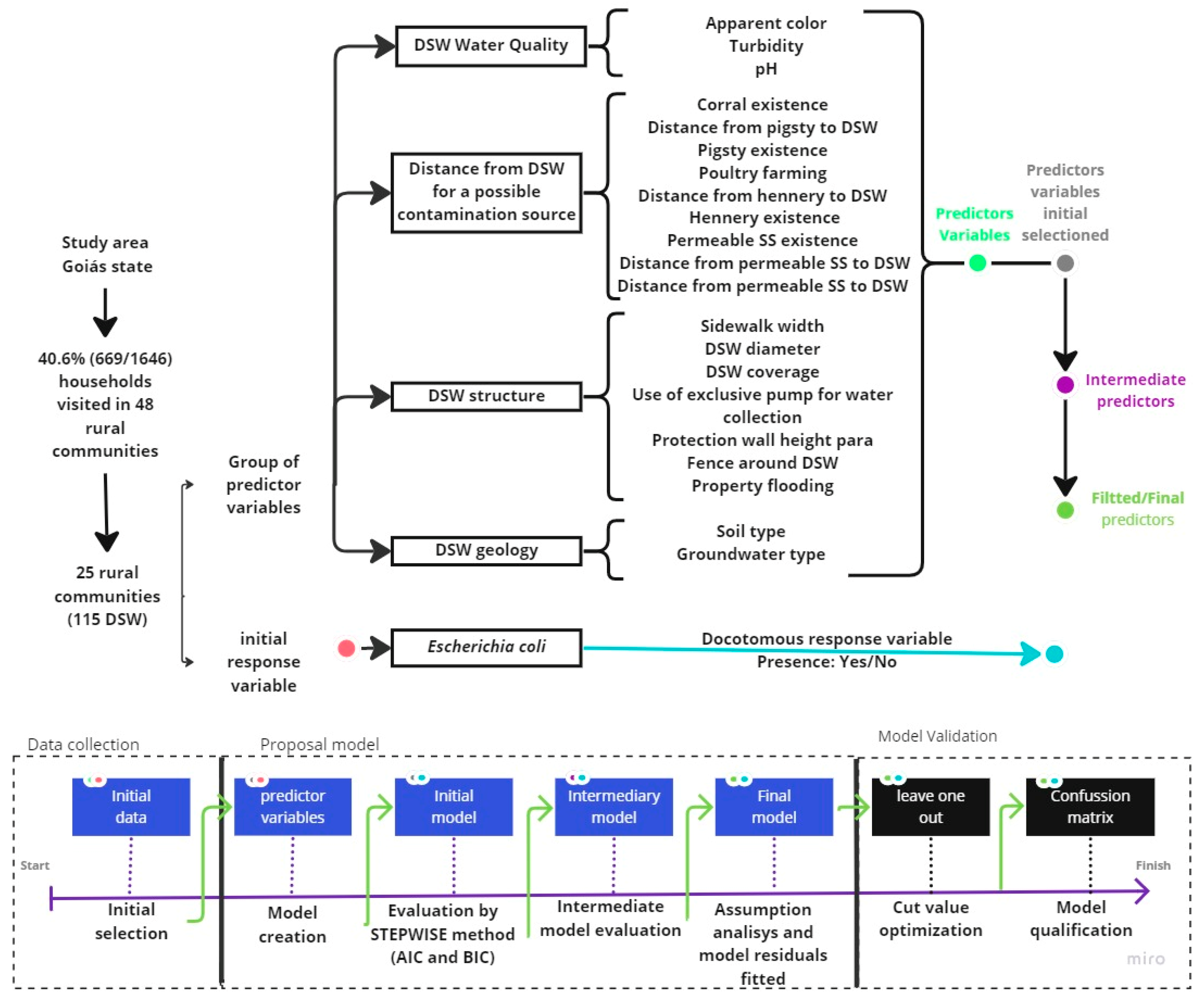
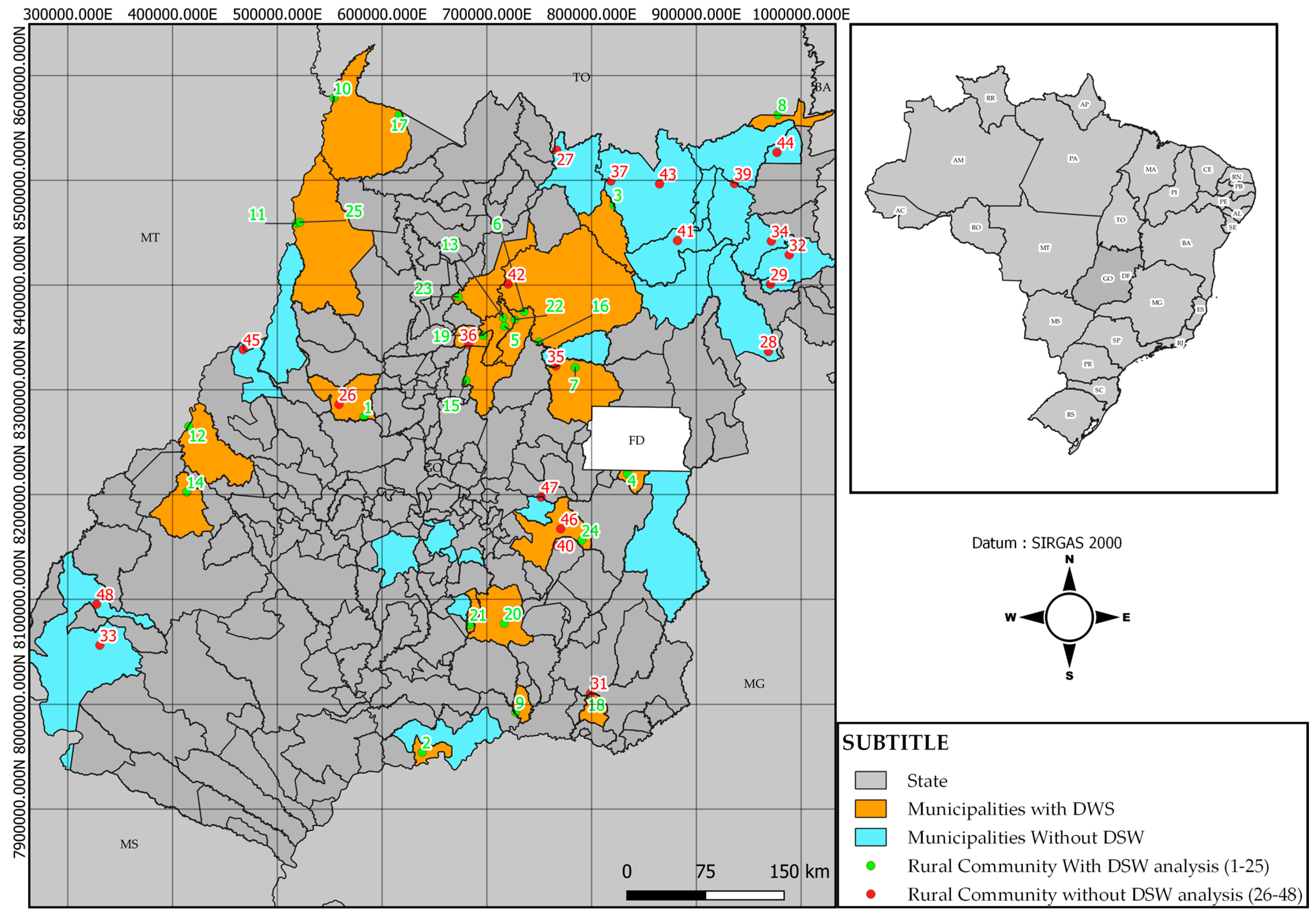
The current research was developed in 48 communities, in the Goiás state of Brazil, in two stages. The first one was the selection of the significant variables among a universe of 23 variables registered in loco. For that, each one was related, pair-by-pair, with the presence/absence of the E. coli variable, selecting those with p-values lower than 0.3 on the statistical test, to then compose the initial model. Subsequently, the variables were evaluated by the stepwise method (Akaike information criterion—AIC and Bayesian information criterion—BIC), aiming to obtain an intermediate model, then a model assumptions analysis was applied, resulting in and confirming the final model. Therefore, the second step was the model validation, performed using the leave-one-out method, thus model performance was evaluated using the confusion matrix, optimizing the cut-off point using the Matthews correlation. In Figure 1, a flowchart describing the present research development can be seen.

2.1. Study Area

The household selection started from 48 rural communities distributed in 36 municipalities (Figure 2), with 40.6% of the households visited (669/1646). Water sources varied in each household, with 37.7% being served using collective solution (from a deep tube well, surface shallow spring, or water eye) and 62.3% using an alternative individual solution (AIS) (14.8% DSW, 7.8% deep tube well, 19.1% shallow excavated well, 3.3% rainwater cistern, 7.8% surface shallow spring, 9.5% water eye). Hence, data from the response variable (Escherichia coli) and the predictive environmental variables (

Table 1. Initial predictive variables identification and characterization to propose a general linear model (GLM).

DSW Water Quality	DSW Estruture	Distance between DSW and a Possible Contamination Source	DSW Geology
Apparent color (1)	Sidewalk width (1)	Distance from the corral to DSW (1)	Soil type (2)
Turbidity (1)	DSW diameter (1)	Corral existence (2)	Groundwater type (2)
pH (1)	DSW coverage (2)	Distance from pigsty to DSW (3)
Total coliforms (1)	Use of exclusive pump for water collection (2)	Pigsty existence (2)
	Protection wall height (1)	Poultry farming (2)
	Fence around DSW (2)	Distance from hennery to DSW (1)
	Property flooding (2)	Hennery existence (2)
		Permeable SS existence (2)
		Distance from permeable SS to DSW (1)
		Distance from permeable SS to DSW (3)

Note: dug shallow wells = DSW; sewage solution = SS; continuous predictor variable = (1); dichotomous predictor variable = (2); ordinal qualitative variable = (3).

) related to 115 DSW, from 128 DSW, were obtained in 25 rural communities located in 22 municipalities in the state of Goiás, Brazil (Figure 2). It must be pointed out that in 13 DSW, it was not possible to obtain all necessary information for analysis, resulting in 115 DSW analyzed, all DSW existing in whole 669 households, from which the geographic coordinates were obtained during data collection, were plotted on a map presented in Supplementary Material Figure S1.

2.2. Data Collection

Data collection was developed in loco from April/2019 to October/2019, cooperatively with the project called Saneamento e Saúde Ambiental em Comunidades Rurais e Tradicionais de Goiás (SanRural). Due to resources and time availability, as well as access to locations, the chosen units were obtained using simple random sampling of a master households’ sample in 17 communities and also by the census in 31 communities, that is, in all households.

Data related to a response variable (Escherichia coli) and 23 predictor variables were collected, being grouped into (i) DSW water quality; (ii) DSW structure; (iii) distance from the DSW to a possible contamination source, and (iv) local geology (Table 1).

Water samples collection and physical-chemical and microbiological analyses were carried out according to standard methods (APHA, AWA, WEF, 2012). Each sample was collected in the discharge pipe before the water arrived at a domestic reservoir when in the pump’s absence, the collection was executed with the aid of a rope and bucket. The samples were stored in flasks packed in a thermal box and transported to the Water Analysis Laboratory (LAnA), located at the School of Civil and Environmental Engineering (EECA) at the Federal University of Goiás (UFG), Goiânia (G), where analyzes were performed.

DSW structural predictor variables: DSW contour sidewalk width, DSW diameter, coverage, the height of the protection wall and depth, way of withdrawing water (manual or pumping), protection fence presence, and possible flooding. The data, as well as the distances from possible contamination sources, were registered in loco, through visual observations and/or mensuration with the aid of measuring tape. The soil and aquifer type were obtained from a free database, provided by the State System of Geoinformation (SIEG) of the state of Goiás, then subsequently processed and analyzed with the aid of the QGIS Software.

2.3. Predictor Variables Initial Selection

The variables (Table 1) were analyzed according to their nature, being classified into three categories: continuous quantitative variables, dichotomous and ordinal qualitative variables. This is due to the fact that there are suitable statistical methods for each kind of variable.

It is relevant to point out that some continuous predictor variables were transformed into ordinal qualitative variables, where intervals recommended in the literature were used, separating them into classes: class 1 (≤100 m), class 2 (>100 m), and absent [28,29,30].

The evaluation between continuous variables and the presence/absence of E. coli was performed using two different methodologies, due to the fact that some variables may be parametric and others non-parametric. Continuous predictor variables were evaluated using the Shapiro-Wilk test (normality test). Variables with normal distribution were submitted to the t-test, while non-parametric variables were studied by the Mann-Whitney test.

The relationships between the qualitative variables and the presence/absence of the E. coli response variable were analyzed using non-parametric independence tests. For this purpose, Fisher’s exact test was applied due to the amount of data (n), based on the hypothesis (h0) that there is the contamination of the DSW due to the applied variable. In both cases, predictive variables with p-values below 0.30 were selected to compose the initial model.

2.4. Model Proposal

GLM is considered a linear model extension, where the data distribution belongs to the exponential distribution families, which can be composed of: normal, binomial, negative binomial, gamma, Poisson, inverse normal, multinomial, beta, logarithmic, among others [31].

In GLM, the dependent variable (response variable y) has a probability density function f represented by Equation (1), where $b(.) e c(.)$ are known functions, meanwhile, $\theta$ e $\Phi$ are parameters.

$$f\left(y;\theta ;\varphi \right)=exp\left\{{\varphi }^{-1}\left[y\theta -b\left(\theta \right)\right]+c\left(y;\varphi \right)\right\}$$

(1)

The density function is expressed in different ways and depends on the response variable assumed distribution.

Table 2. Relationship between the density function and the main distributions belonging to the exponential family.

Distribution	b(θ)	θ	ϕ	$\mathit{c}\left(\mathit{y};\mathit{\varphi }\right)$
Normal (µ,σ2)	θ2/2	µ	σ2	$-\left(\frac{1}{2}\right)\left[\frac{y^2}{{\sigma }^2}+log\left(2\pi {\sigma }^2\right)\right]$
Poisson (µ)	eθ	log(µ)	1	−log(y!)
Binomial (m,$\pi$)	m log(1 + eθ)	log(µ/(m − µ))	1	log$\left(\begin{array}{c}m\\ y\end{array}\right)$
Gama (µ,ν)	−log(−θ)	−1/µ	ν−1	νlog(νy) − log(y) − log($\Gamma \left(\nu \right)$)
Inverse Normal (µ,σ2)	−$\sqrt{-2\theta }$	−1/2µ2	σ2	$-\frac{1}{2}\left[log\left(2\pi {\sigma }^2{y}^3\right)+\frac{1}{{\sigma }^{2}y}\right]$

Note: b(.) e c(.) are known functions, meanwhile, $\theta$, $\Phi$, µ, m, $\pi$, ν, and σ are parameters and $\Gamma (.)$ is gamma function. Font: [31].

shows a summary of the variations attributed to the main distributions belonging to the exponential family.

The relationship between the linear predictor (η), responsible for adhering information to the response variable, and the mean of the variable µ is provided by the link function (g(.)), from equation: $g\left({\mu }_i\right)={\eta }_i$.

Thus, the canonical link function is a particular case of it, in which the canonical parameter (θ) coincides with the linear predictor. It must be noted that each exponential family distribution has its own canonical link function, the main ones are shown in

Table 3. Canonical link function belonging to the main distributions of the exponential family.

Distribution	Normal	Binomial	Poisson	Gama	N. Inverse
Canonical link	µ = η	log{µ/(1 − µ)} = η	logµ = η	µ−1 = η	µ−2 = η

Note: µ is the average of the response variable and η is the linear predictor. Font: [31].

.

The response variable (E. coli) was evaluated according to its distribution with the aid of the easyfit 5.5 software. This software is able to verify more than 50 distribution models from selected data, and its performance is measured by three statistical methods: Kolmogorov-Smirnov, Anderson Darling, and Chi-square. Then the distribution models were ranked according to the p-value obtained.

Subsequently, model selection with the best fit by response variable distribution was executed. It must be emphasized that model creation and all analyzes were performed in Rstudio software.

To assist in choosing the predictor variables to conform to the model, sequential methods were used, in which the most used procedure is the stepwise method, due to its automation and simplicity, in which a sequence of possible models is formed and statistically evaluated until the best combination of predictor variables is found. Hence, to choose the fitted model, four criteria can be used: sum of squared errors, information criterion, partial correlation coefficient, or F statistic.

In the stepwise method, variables can be selected using forward and/or backward selection. In the first case, the method starts only with the intercept (α) and later the predictor variables are added and evaluated until all are used. Subsequently, obtained models are compared and the one that best fits the study is chosen. In the backward selection method, the reverse procedure occurs, in which the model starts full, with all the predictor variables, and later they are removed until they are exhausted.

The stepwise method with Akaike (AIC) and Schwartz (BIC), used in the evaluation of the models, departs from the same principle as the previous ones, however, the objective here is to select a parsimonious model, reducing the number of parameters without taking into account statistical tests, but based on minimum AIC and BIC values.

The Neperian (natural) logarithm model of chance for binomial distribution [32] can be described according to the equation:

$$ln\left(\frac{\mu }{1-\mu }\right)={\beta }_0+{\beta }_1{X}_1+{\beta }_2{X}_2+\cdots +{\beta }_m{X}_m$$

(2)

where: µ indicates the probability that an event will occur; ${\beta }_i$, with i = 1, 2, …, m, are the regression coefficients obtained by likelihood method, X_i the predictor variable, and m is the number of explanatory variables.

Multicollinearity evaluation was developed in the final model, using the variance inflation factor (VIF) and Pearson’s correlation. In both cases, values considered to be strongly correlated with each other were removed from the model, with values greater than 5 for VIF and 0.8 for Pearson’s correlation.

In order to verify the existence of a linear relationship between independent continuous variables with dependent variable logit, the Box-Tindewell test was adopted [33]. Other model assumptions were also verified, which should present mutually exclusive categories, observations independence, and outlier absence. It should be noted that the generated and final model had its residuals analyzed using graphics.

The model fit was evaluated using the Hosmer and Lemeshow method, with the creation of ten groups (G = 10). The null hypothesis refers to a good fit of the model, considering a significance level of 5%.

The probability of occurrence of the event of interest can be formulated by the equation:

$$P\left(Y=1\right)={\left[1+e^{-{(}^{{\beta }_0+{\beta }_1\ast X_1+\cdots +{\beta }_m\ast X_m})}\right]}^{-1}$$

(3)

where: Y = 1 when the event of interest occurs, ${\beta }_i$, with i = 1, 2, …, m, are the regression coefficients obtained by likelihood method, X_i the predictor variable, and m is the number of explanatory variables.

Subsequently, the model is validated by the leave-one-out cross-validation method, in which the model is trained and evaluated, using observations within the research sample universe and predicted data [34].

2.5. Model Validation and Performance

Final model validation was accomplished using the Leave-One-Out cross-validation method, which takes n-1 data from a total of data to train the model and perform the prediction of the nth data. This process is repeated for all variables.

Once the prediction of the n data was performed, the final model performance on predictions was evaluated using the Confusion Matrix. This method evaluates (i) accuracy: the proportion of correct predictions; (ii) sensitivity: the proportion of true positives in relation to positives; (iii) specificity: the presented proportion of true negatives in relation to negatives; (iv) true positive predictors: proportion of true positives in relation to the total number of positive predictions; and (v) true negative predictors: proportion of true negatives compared to the total number of negative predictions.

With the aid of the confusion matrix, it was also possible to optimize the predicted cut-off probability by the final model using the Matthews correlation (MCC). In this process, the cut-off points varied between 0.01 to 0.99 with jumps of 0.01; and for each cut-off point, the Confusion Matrix was calculated and the MCC was derived from it. The chosen cut-off point was the one that maximizes the MCC [35]. both validation and performance calculations were performed using R software with caret package.

3. Results

Considering the results of the response variable and whole 23 predictor variables, obtained for the 115 DSW (supplementary material Table S1) the distribution of continuous and qualitative variables was evaluated, highlighting those where the p-value was less than 0.3, with a total of 13 variables (

Table 4. Statistical analysis result for predictor variables selection to be used in the initial model.

Group of Predictor Variables	Parameter	Normal Distribution	Continuous Variable	Qualitative Variable
		T Student	Mann-Whitney	Fisher
		p-Values	p-Values	p-Values
DSW water quality	Apparent color (1)	NA	0.070 (*)	NA
	Turbidity (1)	NA	0.062 (*)	NA
	pH (1)	0.103 (*)	NA	NA
	Total coliforms (1)	NA	0.000 (*)	NA
DSW Structure	Sidewalk width (1)	NA	0.002 (*)	NA
	DSW depth (1)	NA	0.467	NA
	DSW diameter (1)	NA	0.096 (*)	NA
	Use of exclusive pump for water collection (2)	NA	NA	1
	Protection wall height (1)	NA	0.776	NA
	DSW coverage (2)	NA	NA	0.571
	Fence around DSW (2)	NA	NA	1
	Property flooding (2)	NA	NA	0.395
Distance between DSW and a possible contamination source	Distance from the corral to DSW (1)	NA	0.199 (*)	NA
	Corral existence (2)	NA	NA	0.181 (*)
	Distance from pigsty to DSW (3)	NA	0.803	NA
	Pigsty existence (2)	NA	NA	0.001 (*)
	Poultry farming (2)	NA	NA	0.000 (*)
	Distance from hennery to DSW (1)	NA	0.626	NA
	Hennery existence (2)	NA	NA	0.428
	Distance from permeable SS to DSW (1)	NA	0.654	NA
	Permeable SS existence (2)	NA	NA	0.034 (*)
DSW Geology	Soil type (2)	NA	NA	0.046 (*)
	Groundwater type (2)	NA	NA	0.045 (*)

Note: dug shallow wells = DSW; sewage solution = SS; not applicable = NA; variables selected for the initial model = (*); continuous predictor variable = (1); dichotomous predictor variable = (2); ordinal qualitative variable = (3).

), which were used to propose the initial model.

Among the variables studied, the DSW depth, the use of pumping to remove water from the DSW, the DSW coverage, the DSW protection wall height, the existence of a fence around the DSW, property flooding, the distance from the pigsty to the DSW, the distance from the hennery to the DSW or hennery existence, and the distance from the permeable SS to the DSW, did not compose the initial model because they did not present statistical relationship with the water quality, at a significance level of 0.3, for the studied sample.

3.1. Model Proposal

3.1.1. Initial Model

When evaluating the data distribution of the response variable (E. coli), it was verified that it differed from other evaluated distributions, in which the Pareto generalized distribution was the one that came closest to the values, assuming p-values of 4.971 × 10⁻² and 3.601 × 10⁻³, for the Kolmogorov-Smirnov and Chi-Square tests, respectively. However, the Anderson-Darling test did not calculate a p-value, but a statistical value corresponding to 8.856. However, the R software did not contemplate the generalized Pareto distribution for formulating a GLM. Thus, was chosen to dichotomize the response variable, assuming a binomial distribution, which in turn fits into a logistic regression model.

In

Table 5. Predictive variables selected for the initial model and for the intermediate model indicated as YES according to the AIC and BIC selection criteria.

Group of Predictor Variables	Code	Parameter	Selection Criteria
			AIC	BIC
DSW water quality	AC	Apparent color (1)	No	No
	TURB	Turbidity (1)	Yes	Yes
	pH	pH (1)	No	No
	TC	Total coliforms (1)	No	No
DSW structure	SW	Sidewalk width (1)	Yes	Yes
	DD	DSW diameter (1)	Yes	Yes
Distance between DSW and possible contamination source	Cr	Corral existence (2)	No	No
	Pe	Pigsty existence (2)	Yes	Yes
	Pe class	Distance from pigsty to DSW (3)	No	No
	Po	Poultry farming (2)	Yes	Yes
	SS	Permeable SS existence (2)	No	No
DSW Geology	ST	Soil type (2)	No	No
	GWT	Groundwater type (2)	No	No

Note: sewage solution = SS; continuous predictor variable = (1); dichotomous predictor variable = (2); ordinal qualitative variable = (3); Akaike information criterion = AIC; Bayesian information criterion = BIC; Prioritized variables (highlighted in green).

, it is possible to observe 13 predictor variables selected for the initial model, with six continuous variables, six dichotomous, and one ordinal qualitative. It also presents the five prioritized variables (highlighted in green), both by the AIC and BIC criteria, which will be part of the intermediate predictive model.

3.1.2. Intermediate Model

When the intermediate model was tested, all predictors—DSW diameter (DD), sidewalk width (SW), pigsty existence (Pe), and poultry farming (Po)—showed to be significant, less or equal to 10.0%, excepting turbidity, with 12.73%. In this way, the model could be better fitted without turbidity as a predictor variable, generating an adjusted model with only four predictor variables.

3.1.3. Final Model

Regarding the model multicollinearity, none of the response variables demonstrated a correlation coefficient greater than 0.8. The result for this criterion was confirmed when VIF was estimated, in which all values were less than 5. However, slightly greater than 1 (DD: VIF = 1.073525; SW: VIF = 1.028049; Pe: VIF = 1.063128 and Po: VIF = 1.100042), hence, keeping all predictor variables. Therefore, it is possible to confirm that the predictors used are moderately correlated.

Using the Box-Tindewell method, the present research found for the continuous variables DD and SW, the absence of a linear relationship between independent continuous variables with dependent variable logit at a significance level of 5%, with p-values of 0.526 for DD and 0.758 for SW.

According to the Hosmer and Lemeshow test, the model may be well adjusted, since the null hypothesis was not rejected, with an x² value of 4.1073, and a p-value of 0.8473.

In Figure 3, leverage points or final model influence and its residue are presented, with the aim of verifying the influence of collected observations and adjusting in the generated statistical model.

In the model diagnostic analysis, four sample points were found that are possible leverage points (5, 19, 28, 35), characterized for demonstrating values higher than 2p/n [36], where p is the number of free parameters of the model and n is the sample size. On the other hand, no cases showed Cook’s distance greater than 1 [37], indicating no evidence of influential points. In this way, it was decided not to remove samples fitting the final model, since exclusion points can cause significant changes within the model’s statistical analysis.

In this way, the probability (P) that the DSW is contaminated with E. coli was expressed by Equation (4):

$$P\left(Y=1\right)={\left\{1+e^{-\left[\left(-2.7647)+\left(1.5476\times DD\right)-\left(1.5171\times SW\right)+\left(1.1677\times Pe\right)+(1.4799\times Po\right)\right]}\right\}}^{-1}$$

(4)

where: Y = 1 represents contamination of the DSW by E. coli; DSW diameter = DD; sidewalk width = SW; pigsty existence = Pe; poultry farming = Po.

The model intercept (β₀ at Equation (2)) can be seen in

Table 6. Final model fitted summary.

	Estimate (βm)	Standard Error	Z Value	Pr (>Z)	OR
Intercept (β0)	−2.7647	1.3995	−1.976	0.0482 *	0.0630
DD	1.5476	0.8754	1.768	0.0771 **	4.7001
SW	−1.5171	0.6654	−2.280	0.0226 *	0.2193
Pe	1.1677	0.5256	2.222	0.0263 *	3.2147
Po	1.4799	0.6415	2.307	0.0211 *	4.3925

Note: (*) Significance level between 0.01 and 0.05, (**) significance level between 0.05 and 0.1. DSW diameter = DD; sidewalk width = SW; pigsty existence = Pe; poultry farming = Po; odds ratio = OR.

, as well as regression coefficient estimates (β_m at Equation (2)), the standard error, statistical values for estimates significance analysis, and reasons for chance.

3.2. Model Validation

For final model validation, the cut-off point calculated by the Matthews correlation was used, which generated a value of 0.49. This value means that DSW, through the final model, had a probability greater than 49.0% to be considered contaminated.

When evaluating the reference values (obtained in the experimental phase of this research) the values predicted by the final model composed the confusion matrix, presented in

Table 7. Confusion matrix for the final model.

		Present	Absent
Prediction	Present	83	18
	Absent	2	12

.

In this way, the final model has an adequate accuracy of 82.61%. This reflects its capacity to accurately predict 95 sample points from a sample universe with 115 DSW.

The final model showed good sensitivity since it is capable of predicting the presence of E. coli in 97.65% of cases in which this microorganism is present. On the other hand, the model specificity was 40.0%, indicating its magnitude to predict 40.0% of negative cases that actually exist as negative; therefore, the model omits 60.0% of the negative cases.

However, the final model’s true positive and true negative predictions showed values of 82.18% and 85.71%, respectively. Briefly, 82.18% of positive result predictions are correct and 85.71% of negative result predictions are correct. Both the negative and the positive predictors present important results due to the final model since in the case of organisms that indicate fecal contamination, an error in indicating that a microorganism does not exist in the water from the DSW could represent a risk to consumer health.

4. Discussion

Pairwise evaluation between E. coli presence/absence and the rest of the variables enabled the removal of 10 variables, of which the extracting water method from DSW had no influence. This analysis might be influenced by pumping water removal, observed in 96.5% (111/115) of the DSW, in contrast to the other 3.5% (4/115) characterized water extraction using a bucket. Electric pump and bucket methods were associated with DSW low and high contamination, respectively [38]. Even though the current study demonstrated that DSW depth was not related to E. coli presence, this may happen sometimes [39,40,41], as well as with other variables here studied.

Among all evaluated variables tested in the initial model using the stepwise method, eight variables were removed, with an emphasis on the SS (permeable SS existence) predictor, whose AIC and BIC values were not adequate to keep it in the model. In a similar study, when assessing contamination by E. coli, it was concluded that the microorganism presence was a consequence of another contamination source; therefore, there was no bacteria transport through groundwater flow [2]. In other places, relations between such contamination sources were found [42,43], justifying that the water quality is influenced by underground geological conditions existing in the area [22,44,45]. In this same context, cattle presence (ruminants) near DSW can also influence water quality [42], however, in this study, this variable was discarded to compose the model. For the sample, the universe of the research, the other discarded predictive variables (apparent color, pH, total coliforms, DSW coverage, and distance from pigsty to DSW) were related to water contamination, hence, their variation was not sufficient to predict the probability, or odds ratio, for E. coli presence, in other words, the model can be more efficient when those variables are rejected by the stepwise method.

The proposed model can be used to verify that DSW low chance to be contaminated (0.063). Even in an ideal case, where the absence of pavement (SW) is verified, with very small diameters (DD), drilled in households without pigsty (Pe) and without poultry local farming (Po).

At Jardim Santo Antonio settlement, São Paulo, Brazil, the most related characteristics of contaminated wells were the lid presence and its integrity; gaps between the lid and its entrances; the paving around it and its proximity to contamination sources [2], corroborating the predictive variables found in this research.

DSW diameter variable (Figure 4) had a significant regression coefficient and reflects the increase in the chance of contamination by 4.70001 times, for each 1 meter of horizontal dimension. Although this parameter has a high odds ratio, it does not mean that this parameter mostly influences water quality, since this variable has a low standard deviation, varying in diameter from 1.00 to 4.00 m. It is also noted that of 58 DSW with diameters greater than 1.3 m, 47 contained bacteria in their waters, representing about 81.03%. This situation is relevant and does not imply that DSW with diameters of less than 1.3 m were not contaminated.

On the other hand, for each metric unit of paving (Figure 5) added around DSW, a decrease of 0.2193 times in the chance of contamination is expected, proving that this device is relevant in protecting water against contamination by E. coli. However, their presence should not be disaggregated from other protection devices, since this study is not discussing their efficiency against contamination, but the contamination chances in the studied sample universe.

In the communities, swine farming (Figure 6) proved to be significant for water contamination in DSW, in which the presence of animals in confinement generated a 3.2147-fold increase in the chance that the water was contaminated when compared to the absence of pig farming. This predictor refers only to the mechanism’s existence, disregarding its distances, the number of confined animals, or the existence of effluent management. The results corroborate the occurrence of contamination by E. coli from styes [5,42], as an additional concern of resistant antibiotics organisms [6,46,47], which can be an aggravating factor, since water consumption is common, especially without prior treatment in rural communities.

Similarly, poultry farming in households affects water quality, increasing the chance of contamination 4.3925 times compared with households that do not farm poultry. This situation may be linked to the fact that hens, when free-range, circulate close to the DSW with great ease, in some cases even climbing onto them (Figure 7). This fact can lead to well contamination. A similar result has already been found, where poultry farming was one of the environmental factors promoting a high level of DSW fecal pollution [25,48]. In this way, special attention should be paid to raising these birds without proper management, especially when the water destination from DSW is for human consumption. The presence of microorganisms in chicken feces is a reality, and this is the main reason it is reported in the literature [49,50,51], however, its relationship with water contamination presence is little studied, even though the presence of these birds released in the backyard, or in confinement, is common.

Finally, despite the excellent accuracy of the final model, it cannot predict 100% of the cases and, therefore, it is recommended not to replace water sampling for the purpose of identifying the studied microorganism, but rather be used only for measurements of prioritization and prevention. Furthermore, numerical methods are also prone to errors due to various simplifying assumptions [43,45].

5. Conclusions

With the present study, it was possible to conclude that:

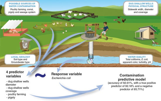
• Shallow well diameter, the paving around it, the presence of pigsties and poultry farming were the predictors that best described (or explained) dug shallow well water contamination;
• For the final model, the pavement in the contour region had a negative relationship with the chance of water contamination of dug shallow wells (OR < 1), and, consequently, there was a probability reduction of water contamination with larger sidewalks, while the well width had a positive relationship (OR > 1), the chance of water contamination was greater in wells with larger diameters when compared to dug shallow wells with small diameters;
• Paving around dug shallow wells can help protect water coming from the well;
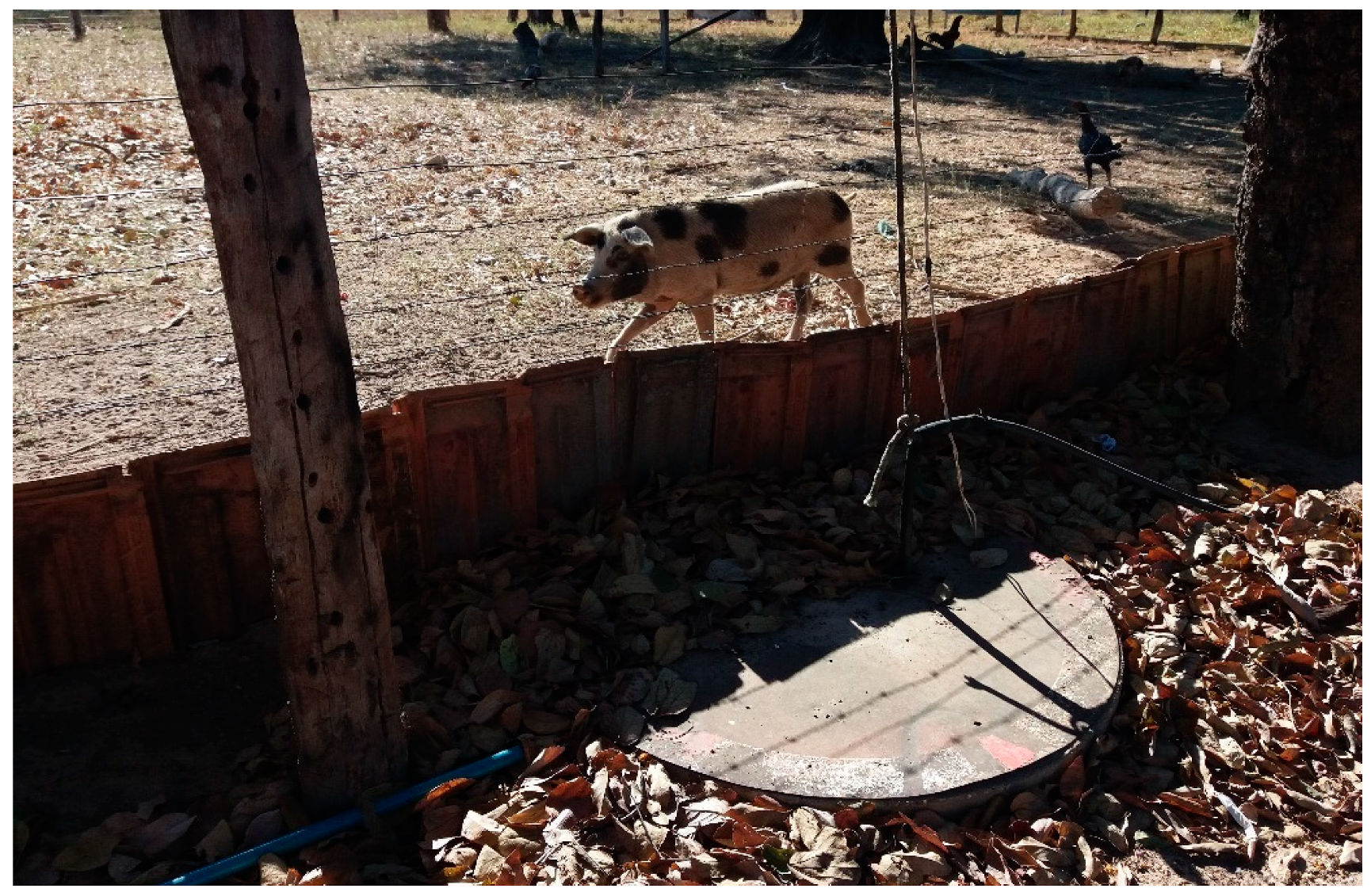
• Rearing pigs and chickens in the peridomicile can harm the quality of the dug shallow wells water;
• The final model showed excellent accuracy in prediction assertiveness.

References

1. Vasconcelos, M.B. What are wells? Overview of the terms used to groundwater abstraction. Águas Subterrâneas 2017, 31, 44–57. [Google Scholar] [CrossRef] [Green Version]
2. Suhogusoff, A.V.; Hirata, R.; Ferrari, L.C.K.M. Water quality and risk assessment of dug wells: A case study for a poor community in the city of São Paulo, Brazil. Environ. Earth Sci. 2013, 68, 899–910. [Google Scholar] [CrossRef]
3. Ocheli, A.; Otuya, O.B.; Umayah, S.O. Appraising the risk level of physicochemical and bacteriological twin contaminants of water resources in part of the western Niger Delta region. Environ. Monit. Assess. 2020, 192, 324–339. [Google Scholar] [CrossRef] [PubMed]
4. Braimah, J.A.; Yirenya-Tawiah, D.R.; Gordon, C. Hand-dug Well Water Quality: The Case of Two Peri-Urban Communities in Ghana. West Afr. J. Appl. Ecol. 2021, 29, 24–34. [Google Scholar]
5. Casey, F.X.M.; Hakk, H.; Desutter, T.M. Free and conjugated estrogens detections in drainage tiles and wells beneath fields receiving swine manure slurry. Environ. Pollut. 2020, 256, 113384. [Google Scholar] [CrossRef] [PubMed]
6. Gao, F.Z.; Zou, H.Y.; Wu, D.L.; Chen, S.; He, L.Y.; Zhang, M.; Bai, H.; Ying, G.G. Swine farming elevated the proliferation of Acinetobacter with the prevalence of antibiotic resistance genes in the groundwater. Environ. Intern. 2020, 136, 105484. [Google Scholar] [CrossRef]
7. Santos, C.E.; Medeiros, R.C.; Mancurso, M.A. Groundwater from rural wells in frederico westphalen: Quality, environmental aspects and legal compliance. An. Do Inst. De Geocienc. 2020, 43, 330–340. [Google Scholar] [CrossRef]
8. Borchardt, M.A.; Stokdyk, J.P.; Kieke, B.A.; Muldoon, M.A.; Spencer, S.K.; Firnstahl, A.D.; Bonness, D.E.; Hunt, R.J.; Burch, T.R. Sources and risk factors for nitrate and microbial contamination of private household wells in the fractured dolomite aquifer of Northeastern Wisconsin. Environ. Health Perspect. 2021, 129, 067004. [Google Scholar] [CrossRef]
9. Wendee, N. Farm to faucet Agricultural waste and private well contamination in Kewaunee county, Wisconsin. Environ. Health Perspect. 2021, 129, 11401. [Google Scholar] [CrossRef]
10. Cherry, J.L. Recent Genetic Changes Affecting Enterohemorrhagic Escherichia coli Causing Recurrent Outbreaks. Microbiol. Spectr. 2022, 10, e00501-22. [Google Scholar] [CrossRef]
11. Abioye, O.M.; Adeniran, K.A.; Abadunmi, T. Poultry Wastes Effect on Water Quality of Shallow Wells of Farms in Two Locations of Kwara State, Nigeria. Nat. Environ. Pollut. Technol. 2022, 21, 303–308. [Google Scholar] [CrossRef]
12. Lwimbo, Z.D.; Komakech, H.C.; Muzuka, A.N.N. Impacts of Emerging Agricultural Practices on Groundwater Quality in Kahe Catchment, Tanzania. Water 2019, 11, 2263. [Google Scholar] [CrossRef] [Green Version]
13. Nyilitya, B.; Mureithi, S.; Boeckx, P. Tracking Sources and Fate of Groundwater Nitrate in Kisumu City and Kano Plains, Kenya. Water 2020, 12, 401. [Google Scholar] [CrossRef] [Green Version]
14. Reynolds, C.; Checkley, S.; Chui, L.; Otto, S.; Neumann, N. Evaluating the risks associated with shiga-toxin-producing Escherichia coli (Stec) in private well waters in Canada. Can. J. Microbiol. 2020, 33, 337–350. [Google Scholar] [CrossRef] [PubMed]
15. Burch, T.R.; Stokdyk, J.P.; Arroz, N.; Andersonanita, C.; Walshjames, F.D.; Spencer, S.K.; Firstahl, A.D.; Borchardt, M.A. Statewide Quantitative Microbial Risk Assessment for Waterborne Viruses, Bacteria, and Protozoa in Public Water Supply Wells in Minnesota. Environ. Sci. Technol. 2021, 56, 6315–6324. [Google Scholar] [CrossRef]
16. Olalemi, A.O.; Ige, O.M.; James, G.A.; Obasoro, F.I.; Okoko, F.O.; Ogunleye, C.O. Detection of enteric bacteria in t w o groundwater sources a n d associated microbial health risks. J. Water Health 2021, 19, 322–335. [Google Scholar] [CrossRef]
17. Chuah, J.C.; Ziegler, A.D. Temporal Variability of Faecal Contamination from On-Site Sanitation Systems in the Groundwater of Northern Thailand. Environ. Manag. 2018, 61, 939–953. [Google Scholar] [CrossRef] [PubMed]
18. Egbueri, J.C.; Ezugwu, C.K.; Ameh, P.D.; Unigwe, C.O.; Ayejoto, D.A. Appraising drinking water quality in Ikem rural area (Nigeria) based on chemometrics and multiple indexical methods. Environ. Monit. Assess. 2020, 192, 308. [Google Scholar] [CrossRef] [PubMed]
19. Lima, F.S.; Scalize, P.S.; Gabriel, E.F.M.; Gomes, R.P.; Gama, A.R.; Demoliner, M.; Spilki, F.R.; Vieira, J.D.G.; Carneiro, L.C. Escherichia coli, Species C Human Adenovirus, and Enterovirus in Water Samples Consumed in Rural Areas of Goiás, Brazil. Food Environ. Virol. 2021, 14, 77–88. [Google Scholar] [CrossRef]
20. Scalize, P.S.; Barros, E.F.S.; Soares, L.A.; Hora, K.E.R.; Ferreira, N.C.; Baumann, L.R.F. Avaliação da qualidade da água para abastecimento no assentamento de reforma agrária Canudos, Estado de Goiás. Rev. Ambient Água 2014, 9, 696–707. [Google Scholar] [CrossRef] [Green Version]
21. Olasoji, S.O.; Oyewole, N.O.; Abiola, B.; Edokpayi, J.N. Water Quality Assessment of Surface and Groundwater Sources Using a Water Quality Index Method: A Case Study of a Peri-Urban Town in Southwest, Nigeria. Environments 2019, 6, 23. [Google Scholar] [CrossRef]
22. Foster, T.; Willetts, J.; Kotra, K.K. Faecal contamination of groundwater in rural Vanuatu: Prevalence and predictors. J. Water Health 2019, 17, 737–748. [Google Scholar] [CrossRef] [PubMed]
23. Park, S.; Kim, J. The Predictive Capability of a Novel Ensemble Tree-Based Algorithm for Assessing Groundwater Potential. Sustainability 2021, 13, 2459. [Google Scholar] [CrossRef]
24. Jenifer, M.A.; Jha, M.K.; Khatun, A. Assessing Multi-Criteria Decision Analysis Models for Predicting Groundwater Quality in a River Basin of South India. Sustainability 2021, 13, 6719. [Google Scholar] [CrossRef]
25. Jang, C.S. Aquifer vulnerability assessment for fecal coliform bacteria using multi-threshold logistic Regression. Environ. Monit. Assess. 2022, 194, 800–815. [Google Scholar] [CrossRef] [PubMed]
26. Kulinkina, A.V.; Sodipo, M.O.; Schultes, O.L.; Osei, B.G.; Agyapong, E.A.; Egorov, A.I.; Naumova, E.N.; Kosinski, K.C. Rural Ghanaian households are more likely to use alternative unimproved water sources when water from boreholes has undesirable organoleptic characteristics. Int. J. Hyg. Environ. Health 2020, 227, 113514. [Google Scholar] [CrossRef] [PubMed]
27. Jang, C.S. Using multi-threshold regression techniques to assess river fecal pollution in the highly urbanized Tamsui River watershed. Environ. Monit. Assess. 2021, 193, 113–126. [Google Scholar] [CrossRef]
28. Otabbong, E.; Arkhipchenko, I.; Orlova, O.; Barbolina, I.; Shubaeva, M. Impact of piggery slurry lagoon on the environment: A study of groundwater and river Igolinka at the Vostochnii Pig Farm, St. Petersburg, Russia. Acta Agric. Scand. B Soil Plant Sci. 2007, 57, 74–81. [Google Scholar] [CrossRef]
29. Tonetti, A.L.; Brasil, A.L.; Madrid, F.J.P.L.; Figueiredo, I.C.S.; Schneider, J.; Cruz, L.M.O.; Duarte, N.C.; Fernandes, P.M.; Coasaca, R.L.; Garcia, R.S.; et al. Tratamento de Esgotos Domésticos em Comunidades Isoladas: Referencial Para a Escolha de Soluções, 1st ed.; Biblioteca/Unicamp: Campinas, SP, Brazil, 2018; 153p. [Google Scholar]
30. Chukwuma, O.M.; Ifeanyichukwu, M.K. Influence of environmental factors on the physico-chemical andbacteriological quality of well and borehole water in rural communities of udenu lga of Enugu State, Nigeria. Pak. J. Nutr. 2018, 17, 596–608. [Google Scholar] [CrossRef]
31. Myers, R.H.; Montgomery, D.C.; Vining, G. Generalized Linear Models: With Applications in Engineering and the Sciences; John Willey: New York, NY, USA, 2012; 520p. [Google Scholar]
32. Sperandei, S. Understanding Logistic Regression Analysis. Biochem. Med. 2013, 24, 12–18. [Google Scholar] [CrossRef]
33. Box, G.E.P.; Tidwell, P.W. Transformation of the Independent Variables. Technometrics 1962, 4, 531–550. [Google Scholar] [CrossRef]
34. Cunha, J.P.Z. Um Estudo Comparativo das Técnicas de Validação Cruzada Aplicadas a Modelos Mistos. Dissertação (Mestrado), Programa de Estatística; Instituto de Matemática e Estatística—Universidade de São Paulo: Butantã, SP, Brazil, 2019; Volume 1, p. 59. [Google Scholar] [CrossRef] [Green Version]
35. Chicco, D.; Jurman, G. The advantages of the Matthews correlation coefficient (MCC) over F1 score and accuracy in binary classification evaluation. BMC Genom. 2020, 21, 6. [Google Scholar] [CrossRef] [PubMed] [Green Version]
36. Belsley, D.A.; Kuh, E.; Welsch, R.E. Regression Diagnostics: Identifying Influential Data and Sources of Collinearity; John Wiley: New York, NY, USA, 1980; 300p. [Google Scholar]
37. Nurunnabi, A.A.R.; Imon, A.H.M.R.; Nasser, M. Identification of multiple influential observations in logistic regression. J. Appl. Stat. 2010, 37, 1605–1624. [Google Scholar] [CrossRef]
38. Machado, A.; Amorim, E.; Bordalo, A.A. Spatial and Seasonal Drinking Water Quality Assessment in a Sub-Saharan Country (Guinea-Bissau). Water 2022, 14, 1987. [Google Scholar] [CrossRef]
39. O’dwyer, J.; Hynds, P.D.; Byrne, K.A.; Ryan, M.P.; Adley, C.C. Development of a hierarchical model for predicting microbiological contamination of private groundwater supplies in a geologically heterogeneous region. Environ. Pollut. 2018, 237, 329–338. [Google Scholar] [CrossRef]
40. Munyebvu, F.; Mujere, N.; Isaac, R.K.; Eslamian, S. Assessing the microbiological quality of potable groundwater from selected protected and unprotected wells in Murehwa district, Zimbabwe. In Advances in Hydrogeochemistry Research, 1st ed.; Nova Science Publishers: New York, NY, USA, 2020; 387p. [Google Scholar]
41. Kazama, S.; Takizawa, S. Evaluation of Microbial Contamination of Groundwater under Different Topographic Conditions and Household Water Treatment Systems in Special Region of Yogyakarta Province, Indonesia. Water 2021, 13, 1673. [Google Scholar] [CrossRef]
42. Malla, B.; Shrestha, R.G.; Tandukar, S.; Bhandari, D.; Inoue, D.; Sei, K.; Tanaka, Y.; Sherchand, J.B.; Haramoto, E. Identificação de Contaminação Fecal Humana e Animal em Fontes de Água Potável no Vale de Kathmandu, Nepal, Usando Ensaios de PCR Quantitativos Bacteroidales Associados ao Hospedeiro. Água 2018, 10, 1796. [Google Scholar] [CrossRef] [Green Version]
43. Díaz-Alcaide, S.; Martínez-Santos, P. Mapping fecal pollution in rural groundwater supplies by means of artificial intelligence classifiers. J. Hydrology 2019, 577, 124006. [Google Scholar] [CrossRef]
44. Wickramasooriya, A.; Gunarathne, S.; Ekanayaka, S. Effect of Subsurface Geological Conditions on Variation of Groundwater Quality in Part of Kurunegala, Sri Lanka; Abrunhosa, M., Chambel, A., Peppoloni, S., Chaminé, H.I., Eds.; Advances in Geoethics and Groundwater Management: Theory and Practice for a Sustainable Development; Springer: Berlin/Heidelberg, Germany, 2021; pp. 233–237. [Google Scholar] [CrossRef]
45. Nasir, M.J.; Tufail, M.; Ayaz, T.; Khan, S.; Khan, A.Z.; Lei, M. Groundwater quality assessment and its vulnerability to pollution: A study of district Nowshera, Khyber Pakhtunkhwa, Pakistan. Environ. Monit. Assess. 2022, 194, 692–719. [Google Scholar] [CrossRef]
46. He, L.Y.; Ying, G.G.; Liu, Y.S.; Su, H.C.; Chen, J.; Liu, S.S.; Zhao, J.L. Discharge of swine wastes risks water quality and food safety: Antibiotics and antibiotic resistance genes from swine sources to the receiving environments. Environ. Int. 2016, 92–93, 210–219. [Google Scholar] [CrossRef]
47. Brisola, M.C.; Crecencio, R.B.; Bitner, D.S.; Frigo, A.; Rampazzo, L.; Stefani, L.M.; Faria, G.A. Escherichia coli used as a biomarker of antimicrobial resistance in pig farms of Southern Brazil. Sci. Total Environ. 2019, 647, 362–368. [Google Scholar] [CrossRef] [PubMed]
48. Lu, Y.; Philp, R.P.; Biache, C. Assessment of Fecal Contamination in Oklahoma Water Systems through the Use of Sterol Fingerprints. Environments 2016, 3, 28. [Google Scholar] [CrossRef] [Green Version]
49. Amir, M.; Riaz, M.; Chang, Y.-F.; Ismail, A.; Hameed, A.; Ahsin, M. Antibiotic Resistance in Diarrheagenic Escherichia coli Isolated from Broiler Chickens in Pakistan. J. Food Qual. Hazards Control 2021, 8, 78–86. [Google Scholar] [CrossRef]
50. van den Bogaard, A.E.; Londres, N.; Driessen, C.; Stobberingh, E.E. Antibiotic resistance of faecal Escherichia coli in poultry, poultry farmers and poultry slaughterers. J. Antimicrob. Chemother. 2021, 47, 763–771. [Google Scholar] [CrossRef]
51. Bamidele, O.; Yakubu, A.; Joseph, E.B.; Amole, T.A. Antibiotic Resistance of Bacterial Isolates from Smallholder Poultry Droppings in the Guinea Savanna Zone of Nigeria. Antibiotics 2022, 11, 973. [Google Scholar] [CrossRef] [PubMed]
Figure 1. Flowchart of the methodology used in the present research.
Sustainability 15 02408 g001
Figure 2. Location of communities participating in presente study. Note: Água Limpa community = (1); Córrego do Inhambú community = (2), José de Coleto community = (3), Mesquita community = (4), Pombal community = (5), Fazenda Santo Antônio da Laguna community = (6), Sumidouro community = (7), Taquarussu community = (8), Arraial da Ponte = (9), Fio Velasco = (10), Landi = (11), Registro do Araguaia = (12), Engenho da Pontinha = (13), Fortaleza = (14), Itajá II = (15), Julião Ribeiro = (16), Lageado = (17), Madre Cristina = (18), Monte Moriá = (19), Piracanjuba = (20), Rochedo = (21), Santa Fé da Laguna = (22), São Lourenço = (23), São Sebastião = (24), Tarumã = (25), Arraial da Antas II = (26), Céu Azul = (27), Canabrava community = (28), Castelo/Retiro e Três Rios community = (29), Pelotas community = (30), Povoado Veríssimo = (31), Baco Pari community = (32), Cedro community = (33), Extrema community = (34), Mimoso community = (35), Porto Leocádio community = (36), Quilombo de Minaçu community = (37), Forte community = (38), Quilombo do Magalhães community = (39), Almeidas community = (40), Povoado Moinho community = (41), Rafael Machado community = (42), São Domingos community = (43), Vazante community = (44), Itacaiú = (45), João de Deus (46), Olho d’Agua = (47), Pouso Alegre = (48).
Sustainability 15 02408 g002
Figure 3. Diagnosis graph for final model, residual vs fitted values (a); normal Q-Q (b); standardized Pearson residue (c); cook’s distance (d).
Sustainability 15 02408 g003
Figure 4. DSW illustration with smaller (a) and larger (b) diameter.
Sustainability 15 02408 g004
Figure 5. DSW illustration with smaller (a) and larger (b) shoes.
Sustainability 15 02408 g005
Figure 6. Household with extensive swine rearing illustration, with DSW close to circulation areas.
Sustainability 15 02408 g006
Figure 7. DSW illustration with smaller (a) and larger (b) shoes with contamination.
Sustainability 15 02408 g007