
Frequency Regulation for State-Space Model-Based Renewables Integrated to Multi-Area Microgrid Systems


Abstract
:1. Introduction
- Derivation of SS models for solar and wind systems for the given specifications.
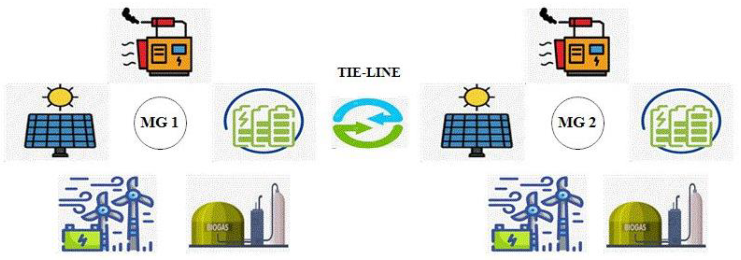
- Development of identical two area microgrid model fed with standard functions for DEG, BGP, and BESS.
- The proposed higher degree polynomials of PV and wind are inserted into the system for rigorous testing of its behavior and impact.
- Simultaneous operation of different controllers such as PID, FOPID, 2DOF-FOPID, and 3DOF-FOPID controller in both the areas.
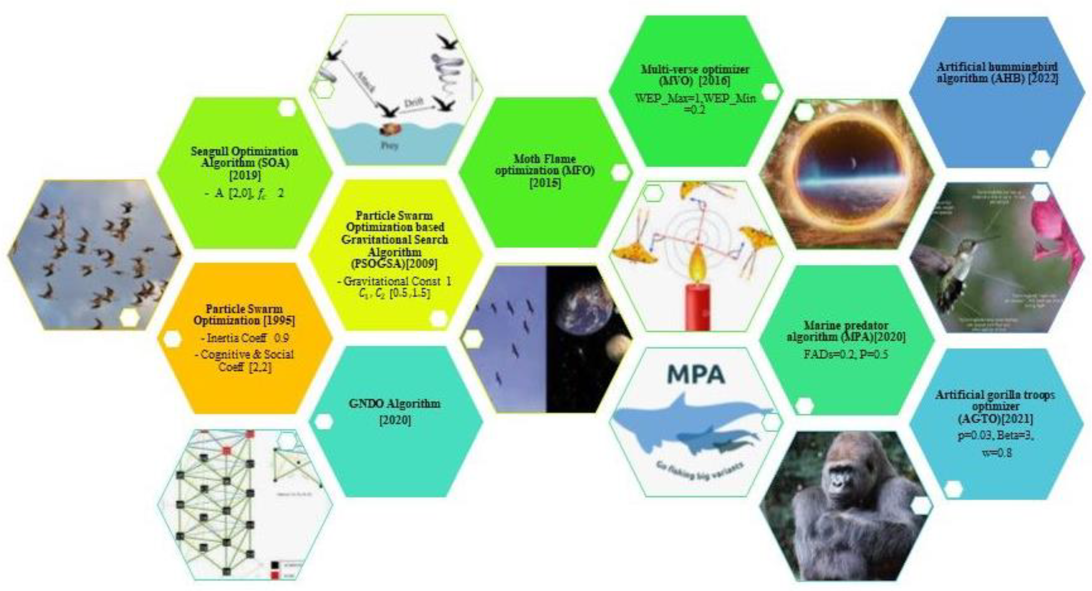
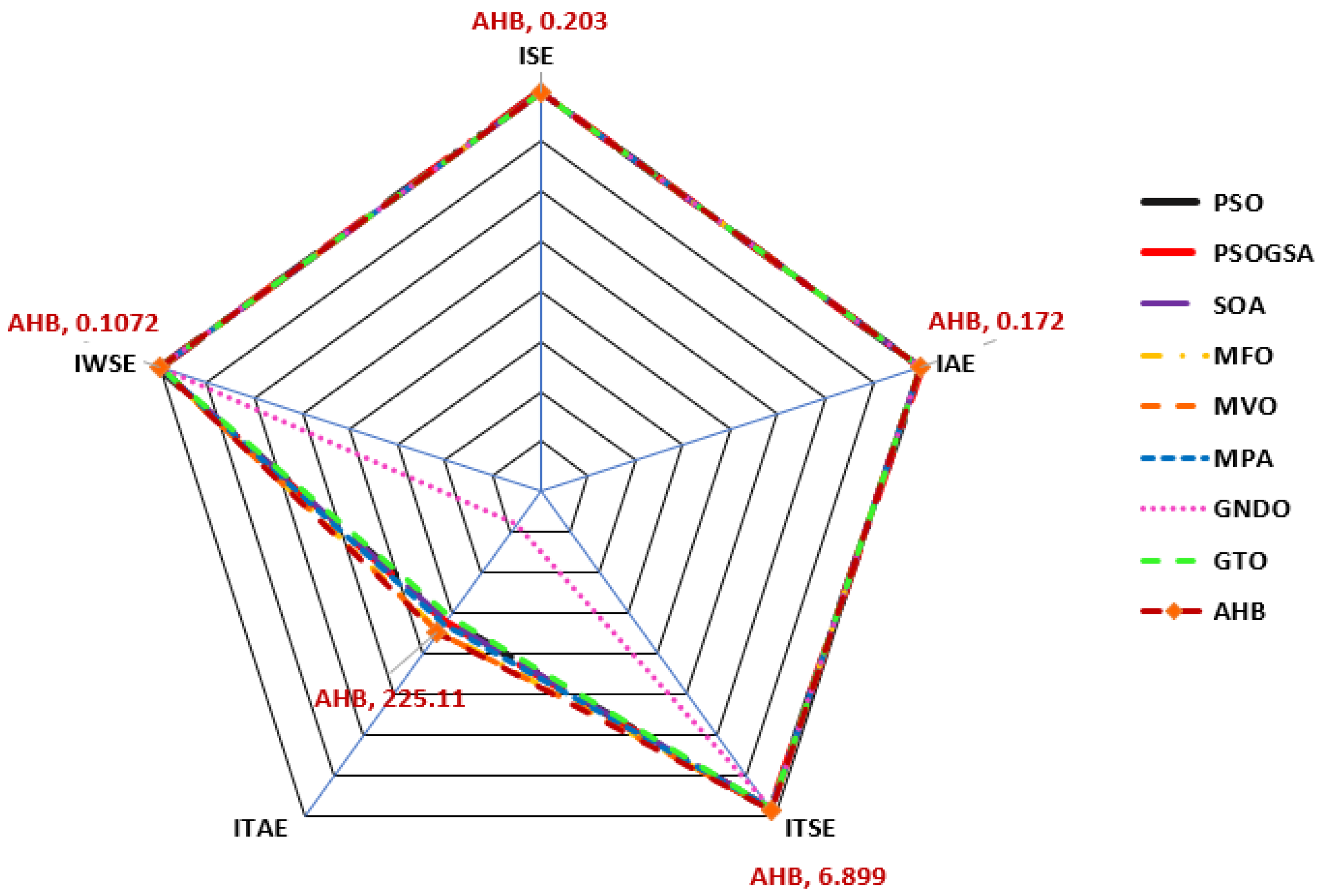
- Proposed network subjected to step perturbations and compared with PSO, PSO-GSA, SOA, MFO, MVO, MPA, GNDO, and GTO. The evident simulation results justify the proposed system to be more preferable when compared with the existing stigma.
- Procuring transient and sensitivity analysis under thermal constraints (GRC, GDB) and variable operating conditions (±25%, ±50% tolerance), respectively, which confines the feasibility and compatibility of the proposed network.
2. Microgrid System Model
2.1. Discrete Representation of the Components
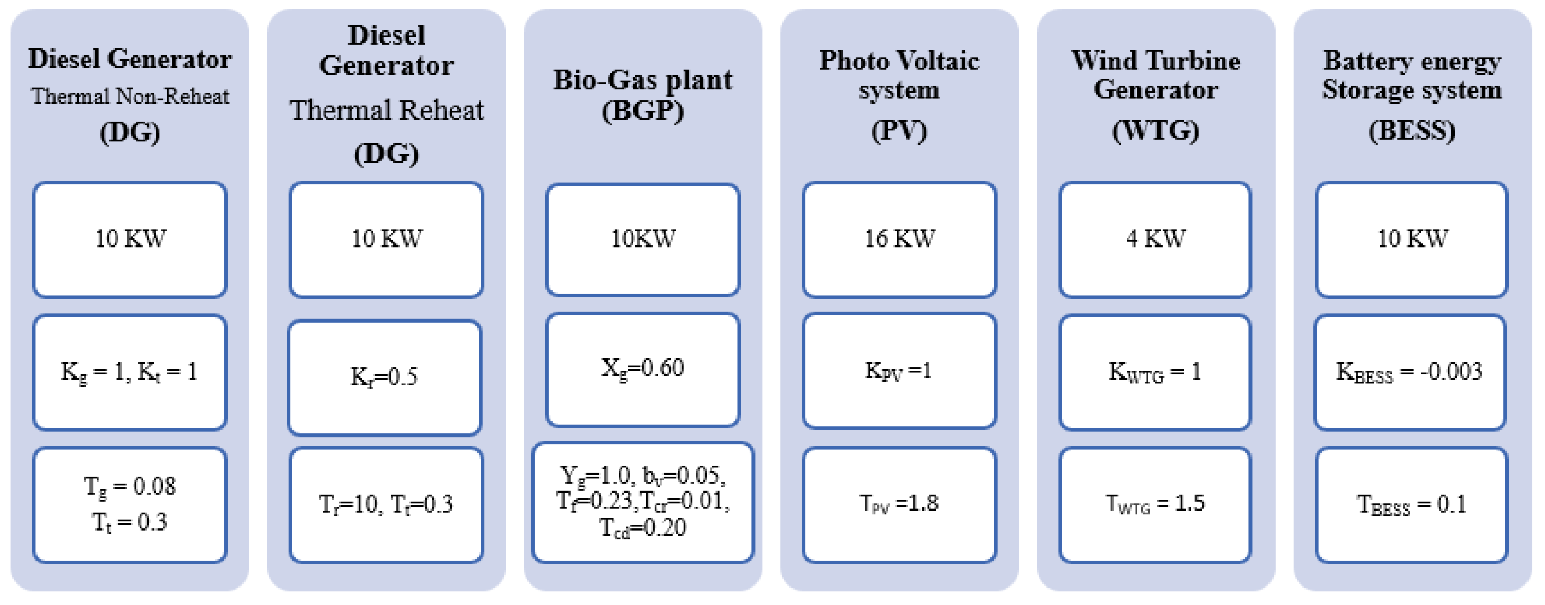
2.1.1. Diesel Engine Generator (DEG)
2.1.2. Biogas Plant (BGP) Model
2.1.3. Battery Energy Storage Systems (BESS)
2.1.4. Load Model
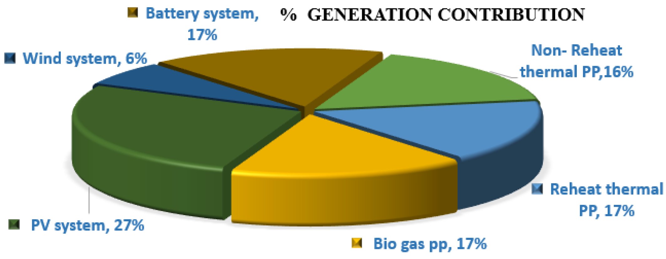
2.1.5. Power Model
2.1.6. Renewable Integration Models
2.2. SS Formation of Renewables
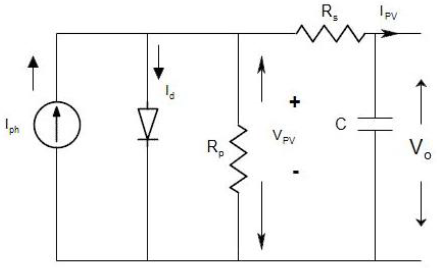
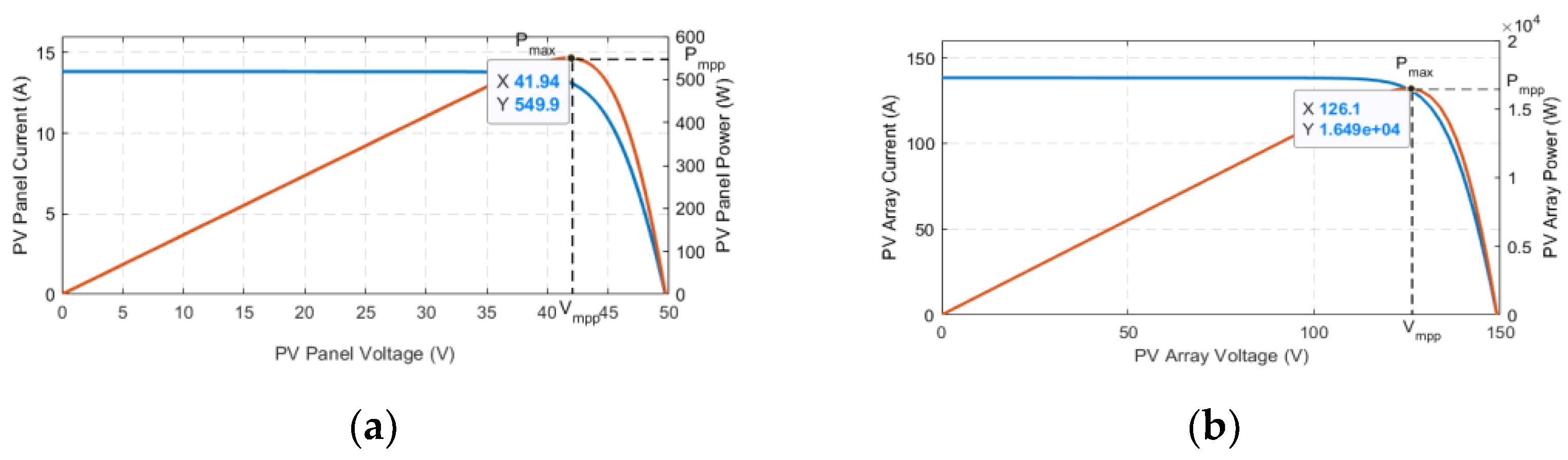
2.2.1. PV System
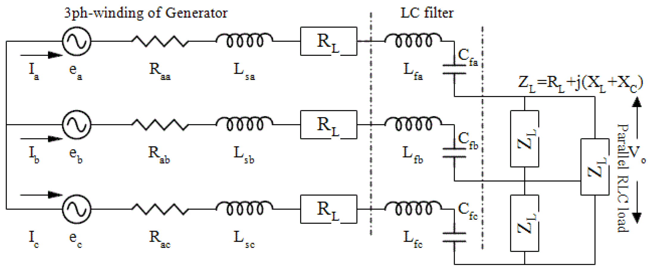
2.2.2. Wind System
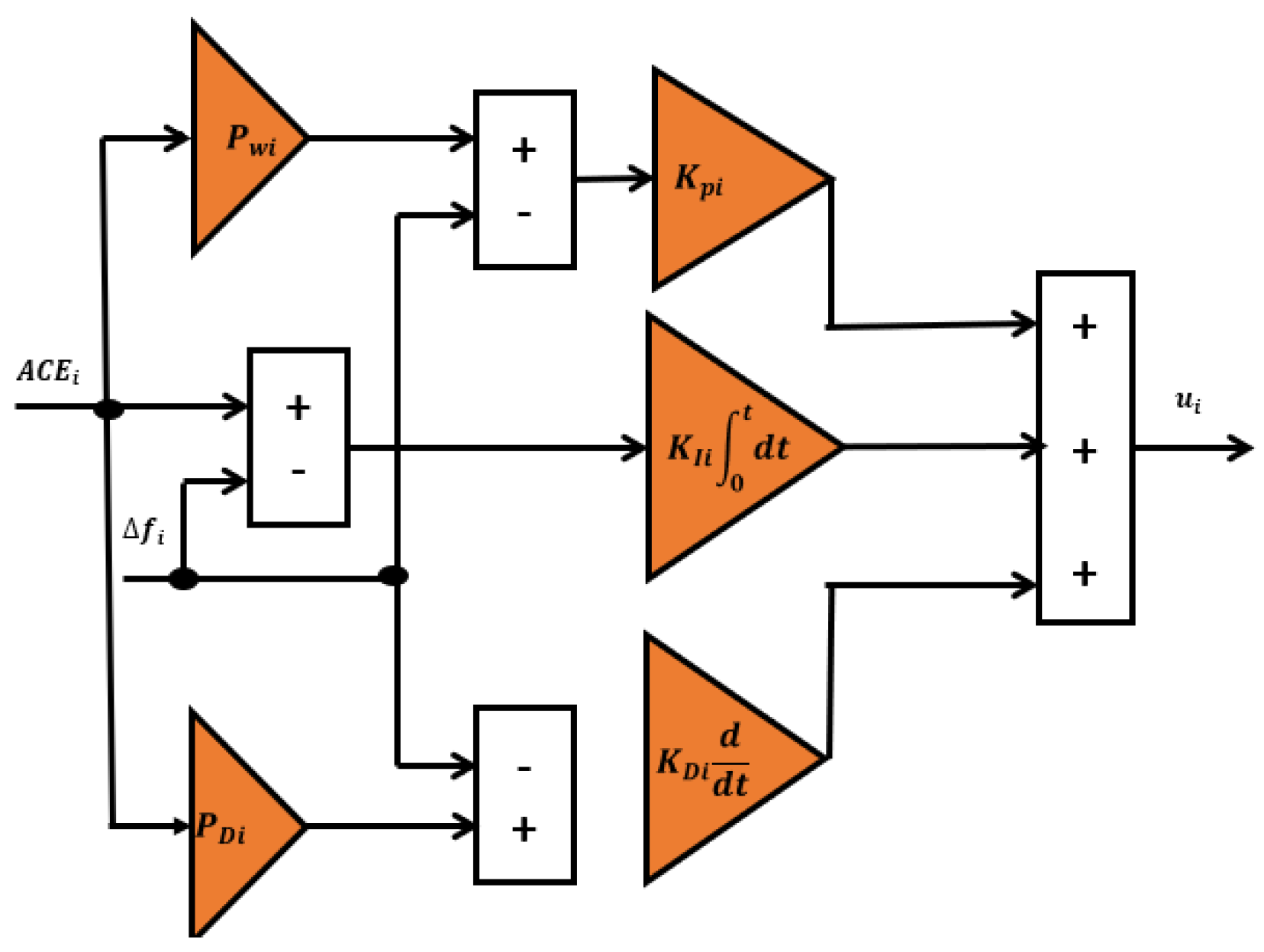
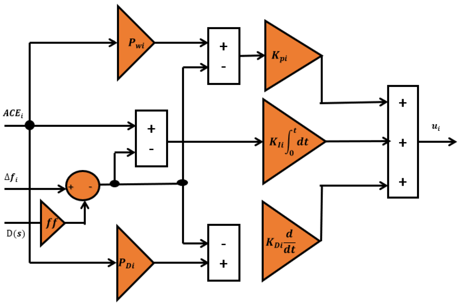
3. Summary of Two and Three Stage FOPID Controllers
4. Skeletal of Anticipated Heuristic Approach
4.1. Initialization
4.2. Guided Foraging
4.3. Territorial Foraging
4.4. Migration Foraging
5. Investigations and Discussions
5.1. Transient Analysis
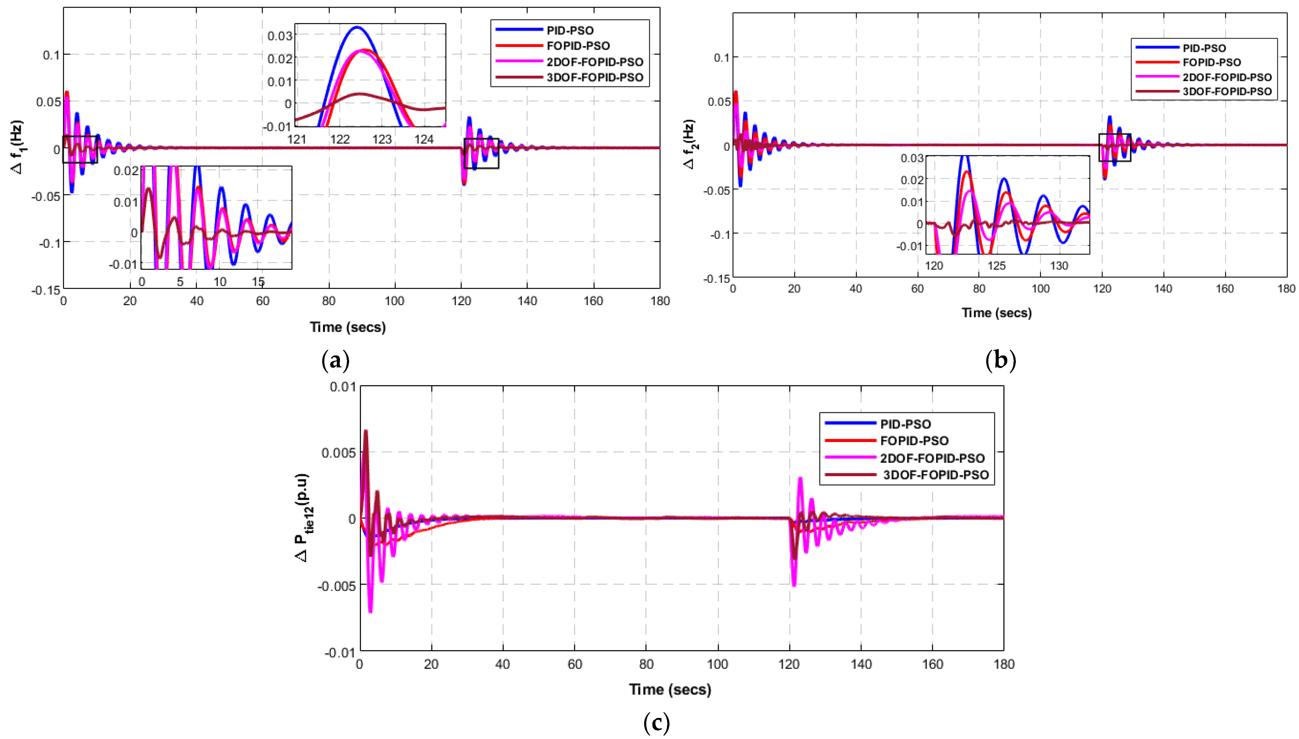
5.1.1. Assessment of Multi-Microgrid with Single-Step Load Disturbance in Area 1
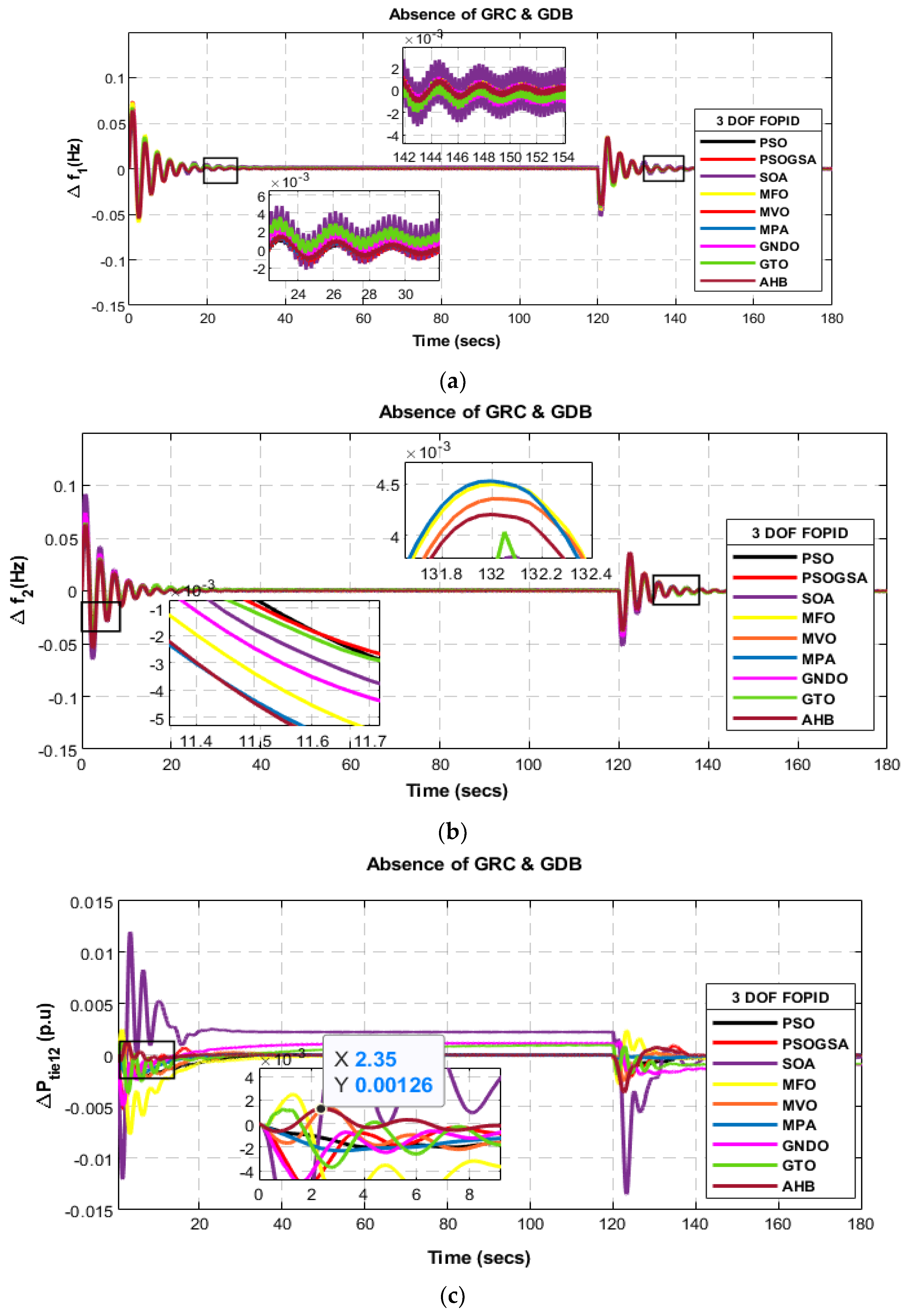
5.1.2. Assessment with the Modern Heuristic Method in the Absence of Constraints
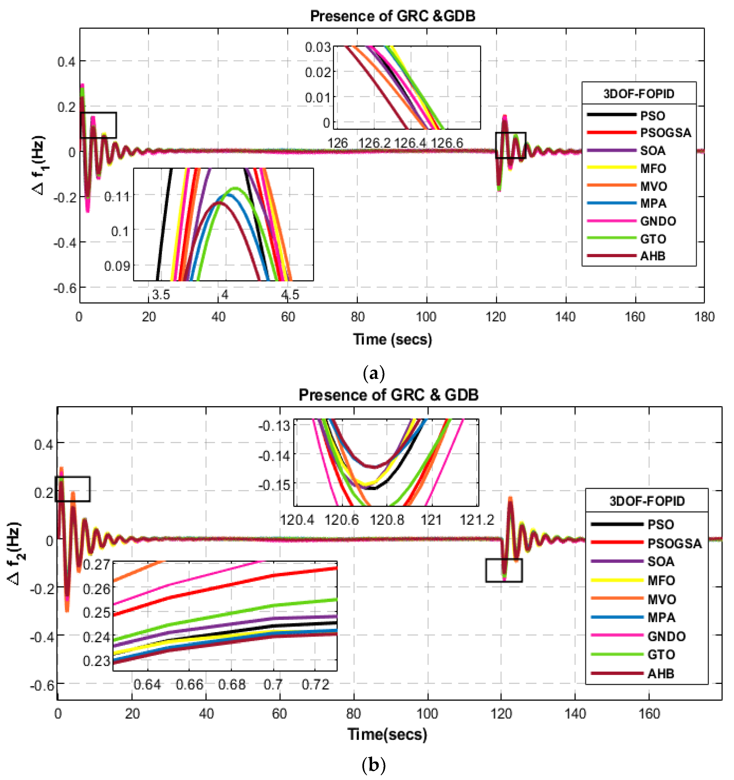
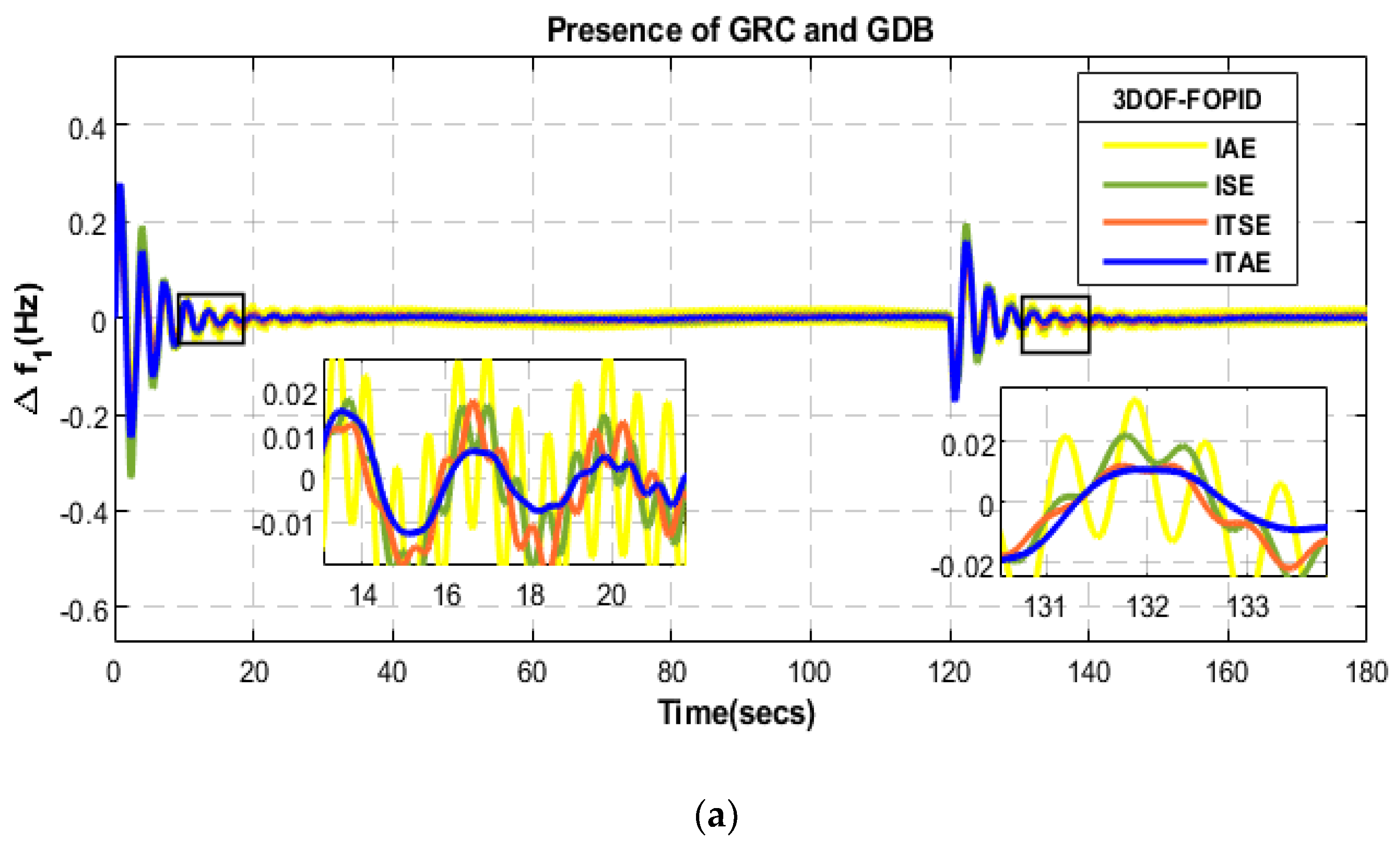
5.1.3. Valuation with the Modern Heuristic Method in the Presence of GRC and GDB
5.1.4. Effect of Multi-step Disturbance in Realization of Response
5.2. Sensitivity Analysis
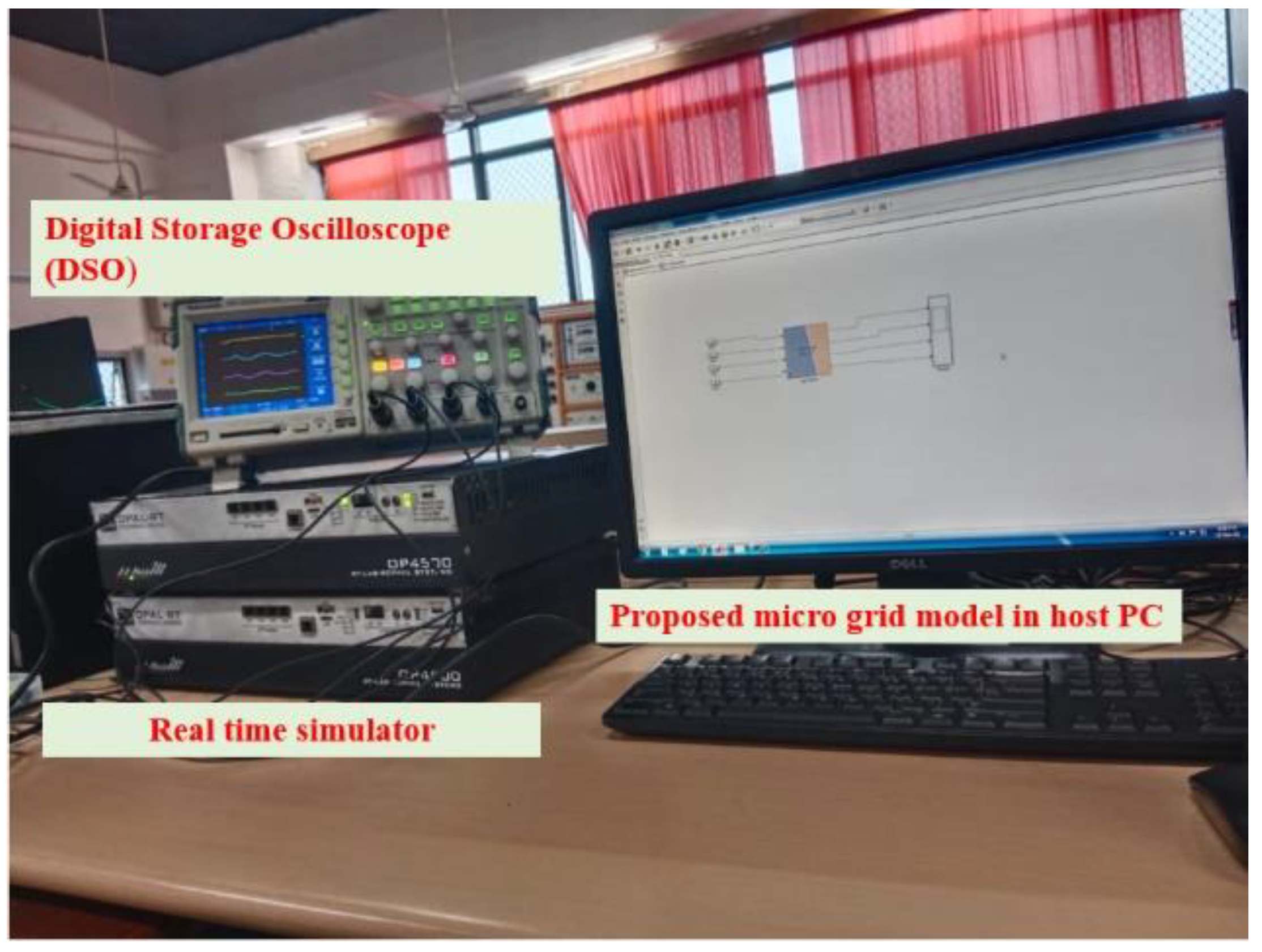
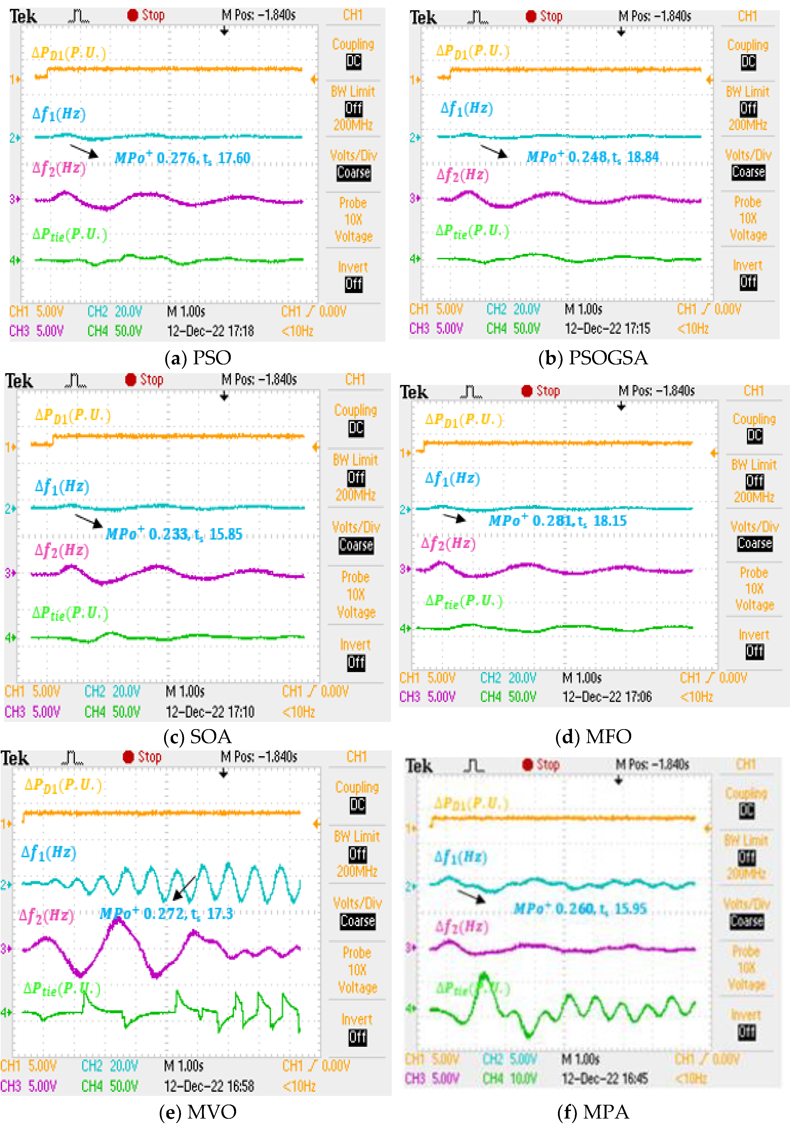
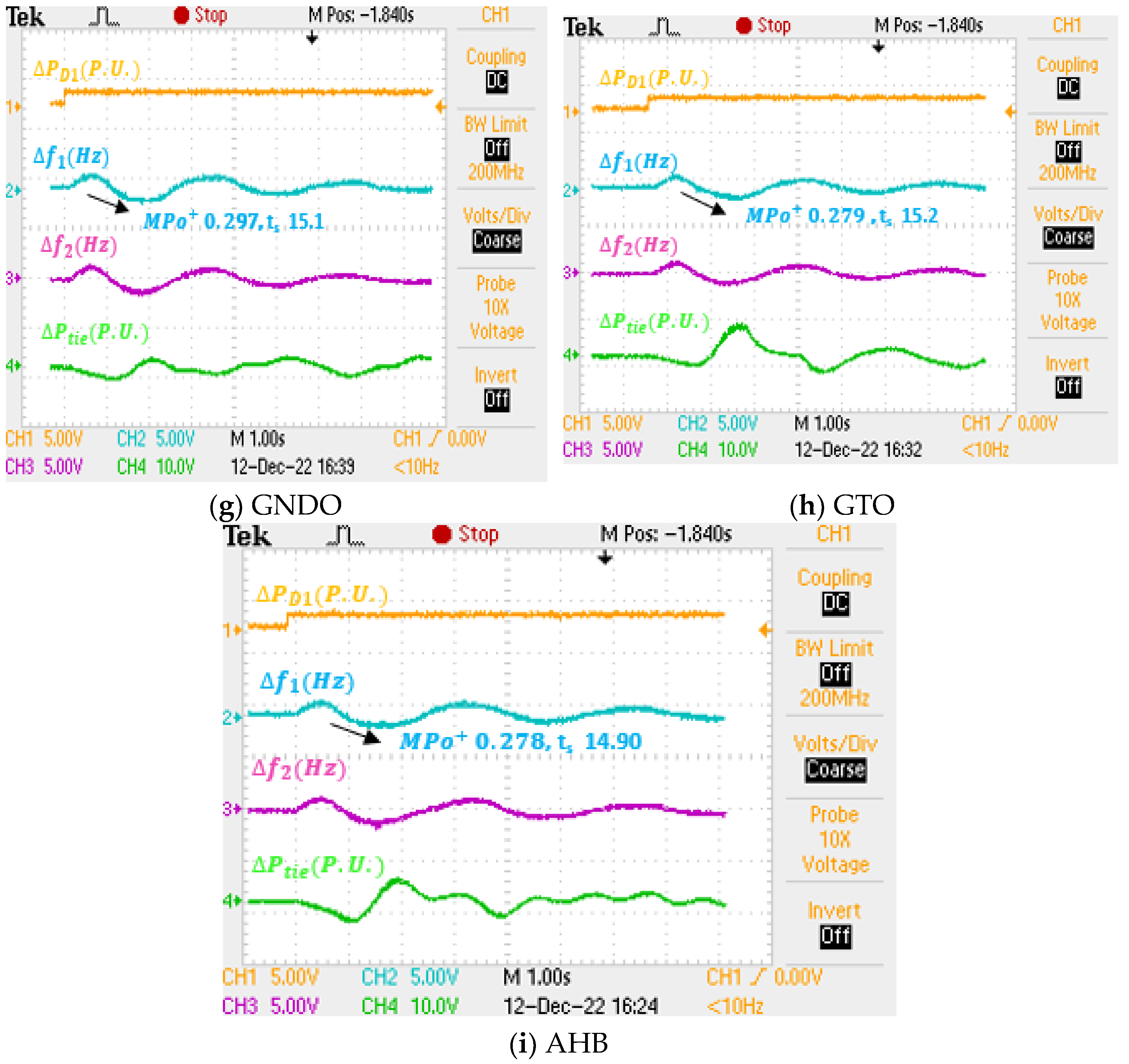
6. Experimental Authentication in Real-Time Simulator
7. Conclusions
8. Future Recommendations
Author Contributions
Funding
Institutional Review Board Statement
Informed Consent Statement
Data Availability Statement
Acknowledgments
Conflicts of Interest
Abbreviations
| i | subscript refers to the ith area |
| ∆f | frequency change (Hz) |
| ∆fi | system frequency deviation (Hz) in area i |
| ∆Ptie | Incremental change in tie-line power (p.u) |
| Kps, Tps | Gain and Time constant of the power system model |
| KBESS, TBESS | Gain and Time constant of the battery energy storage system |
| KPV, TPV | Solar system gain and Time constant |
| KWTG, TWTG | Gain and Time constant of the wind turbine generator |
| Kg, Tg | Governor constant |
| Kt, Tt | Turbine constant |
| ∆PD | change in load (p.u) |
| Pri | Rated power of the area i (KW) |
| ajj | = −(Pri/Prj) |
| Ri | Speed regulation of area i (Hz/pu KW) |
| Bi | frequency bias coefficient of area i (pu KW/Hz) |
| Hi | Inertia constant (secs) of control area i |
| Π | =pi |
| KPi, KIi,KDi | controller gain constants at ith area |
| ACEi | area control error of ith area |
| ∆PBESS | Incremental output power of BESS (p.u) |
| ∆PDEG,NR & ∆PDEG, R | Incremental power of DEG with non-reheat and reheat turbine (p.u) |
| ∆PPV | Incremental solar power (p.u) |
| ∆PBGP | change in bio-gas power (p.u) |
| Φ | Irradiation (W/m2) |
| βi | area frequency response characteristic (AFRC) (p.u KW/Hz) |
| J | fitness function or FOD |
| Kmin, Kmax | lower and upper bound of gain |
| Xg, Yg | Time constants of lead and lag |
| bv,Tcd | Bio-gas unit valve actuator and discharge delay |
| Tcr,Tf | Delay in combustion reaction and bio-gas |
| ±δ | 3% minute |
| N1,N2 | 0.8, −0.2 Π |
| I, PI | Integral, Proportional-Integral |
| PID | Proportional-Integral-Derivative |
| FOPID | Fractional Order PID |
| 2DOF and 3DOF FOPID | Two Degree of Freedom and Three Degree of Freedom-based FOPID |
| DSO | Digital Storage Oscilloscope |
References
- Arya, Y. A new optimized fuzzy FOPI-FOPD controller for automatic generation control of electric power systems. J. Frankl. Inst. 2019, 356, 5611–5629. [Google Scholar] [CrossRef]
- Gozde, H.; Taplamacioglu, M.C.; Kocaarslan, I. Comparative performance analysis of Artificial Bee Colony algorithm in automatic generation control for interconnected reheat thermal power system. Int. J. Electr. Power Energy Syst. 2012, 42, 167–178. [Google Scholar] [CrossRef]
- Chen, G.; Li, Z.; Zhang, Z.; Li, S. An Improved ACO Algorithm Optimized Fuzzy PID Controller for Load Frequency Control in Multi-Area Interconnected Power Systems. IEEE Access 2020, 8, 6429–6447. [Google Scholar] [CrossRef]
- Pappachen, A.; Fathima, A.P. NERC’s control performance standards-based load frequency controller for a multi area deregulated power system with ANFIS approach. Ain Shams Eng. J. 2017, 9, 2399–2414. [Google Scholar] [CrossRef]
- Doley, R.; Ghosh, S. Application of PID and fuzzy based controllers for load frequency control of a single-Area and double-Area power systems. In Proceedings of the 2019 5th International Conference on Advances in Electrical Engineering (ICAEE), Dhaka, Bangladesh, 26–28 September 2019; pp. 479–484. [Google Scholar] [CrossRef]
- Prakash, A.; Kumar, K.; Parida, S.K. PIDF (1+FOD) controller for load frequency control with sssc and ac-dc tie-line in deregulated environment. IET Gener. Transm. Distrib. 2020, 14, 2751–2762. [Google Scholar] [CrossRef]
- Rahman, A.; Saikia, L.C.; Sinha, N. Load frequency control of a hydro-thermal system under deregulated environment using biogeography-based optimized three-degree-of-freedom integral-derivative controller. IET Gener. Transm. Distrib. 2015, 9, 2284–2293. [Google Scholar] [CrossRef]
- Shiva, C.K.; Mukherjee, V. Automatic generation control of multi-unit multi-area deregulated power system using a novel quasi-oppositional harmony search algorithm. IET Gener. Transm. Distrib. 2015, 9, 2398–2408. [Google Scholar] [CrossRef]
- Mohanty, B.; Hota, P.K. Comparative performance analysis of fruit fly optimization algorithm for multi-area multisource automatic generation control under deregulated environment. IET Gener. Transm. Distrib. 2015, 9, 1845–1855. [Google Scholar] [CrossRef]
- Tasnin, W.; Saikia, L.C. Performance comparison of several energy storage devices in deregulated AGC of a multi-area system incorporating geothermal power plant. IET Renew. Power Gener. 2018, 12, 761–772. [Google Scholar] [CrossRef]
- Gupta, M.; Gupta, S.; Thakur, T. Implementation of new electricity regulatory norms for deviation settlement mechanism: A case study of India. Cogent Eng. 2019, 6, 1623152. [Google Scholar] [CrossRef]
- Lakshmi, D.; Fathima, A.P.; Muthu, R. Simulation of the two-area deregulated power system using particle swarm optimization. Int. J. Electr. Eng. Inform. 2016, 8, 93–107. [Google Scholar] [CrossRef]
- Veronica, A.J.S.J.; Kumar, N.S.; Gonzalez-Longatt, F. Robust PI controller design for frequency stabilization in a hybrid microgrid system considering parameter uncertainties and communication time delay. IET Gener. Transm. Distrib. 2019, 13, 3048–3056. [Google Scholar] [CrossRef]
- Raju, M.; Saikia, L.C.; Sinha, N. Load frequency control of multi-area hybrid power system using symbiotic organisms search optimized two degree of freedom controller. Int. J. Renew. Energy Res. 2017, 7, 1664–1674. [Google Scholar]
- Ganthia, B.; Rout, K. Deregulated power system-based study of AGC using PID and fuzzy logic controller. Int. J. Adv. Res. 2016, 4, 847–855. [Google Scholar] [CrossRef] [Green Version]
- Donde, V.; Pai, M.A.; Hiskens, I.A. Simulation and optimization in an AGC system after deregulation. IEEE Trans. Power Syst. 2001, 16, 481–489. [Google Scholar] [CrossRef]
- Wang, X.; Zhao, Q.; He, B.; Wang, Y.; Yang, J.; Pan, X. Load frequency control in multiple microgrids based on model predictive control with communication delay. J. Eng. 2017, 2017, 1851–1856. [Google Scholar] [CrossRef]
- Latif, A.; Das, D.C.; Ranjan, S.; Barik, A.K. Comparative performance evaluation of WCA-optimised non-integer controller employed with WPG–DSPG–PHEV based isolated two-area interconnected microgrid system. IET Renew. Power Gener. 2019, 13, 725–736. [Google Scholar] [CrossRef]
- Khooban, M.H.; Dragicevic, T.; Blaabjerg, F.; Delimar, M. Shipboard Microgrids: A Novel Approach to Load Frequency Control. IEEE Trans. Sustain. Energy 2018, 9, 843–852. [Google Scholar] [CrossRef]
- Yammani, C.; Maheswarapu, S. Load Frequency Control of Multi-microgrid System considering Renewable Energy Sources Using Grey Wolf Optimization. Smart Sci. 2019, 7, 198–217. [Google Scholar] [CrossRef]
- Khooban, M.H.; Niknam, T.; Shasadeghi, M.; Dragicevic, T.; Blaabjerg, F. Load Frequency Control in Microgrids Based on a Stochastic Noninteger Controller. IEEE Trans. Sustain. Energy 2018, 9, 853–861. [Google Scholar] [CrossRef]
- Poulose, A.; Kumar, R.P. Higher Order Sliding Mode Controller-Based Load Frequency Control for a Two-Area Interconnected Power System. Master’s Thesis, Department of Electrical Engineering, Government Engineering College, Maharashtra, India, 2019. [Google Scholar] [CrossRef]
- Veerasamy, V.; Wahab, N.I.A.; Ramachandran, R.; Othman, M.L.; Hizam, H.; Irudayaraj, A.X.R.; Guerrero, J.M.; Kumar, J.S. A Hankel Matrix Based Reduced Order Model for Stability Analysis of Hybrid Power System Using PSO-GSA Optimized Cascade PI-PD Controller for Automatic Load Frequency Control. IEEE Access 2020, 8, 71422–71446. [Google Scholar] [CrossRef]
- Ebrahim, M.A.; Aziz, B.A.; Nashed, M.N.F.; Osman, F.A. A Novel Hybrid-HHOPSO Algorithm based Optimal Compensators of Four-Layer Cascaded Control for a New Structurally Modified AC Microgrid. IEEE Access 2020, 9, 4008–4037. [Google Scholar] [CrossRef]
- Barik, A.K.; Das, D.C. Proficient load-frequency regulation of demand response supported bio-renewable cogeneration-based hybrid microgrids with quasi-oppositional selfish-herd optimization. IET Gener. Transm. Distrib. 2019, 13, 2889–2898. [Google Scholar] [CrossRef]
- Barik, A.K.; Jaiswal, S.; Das, D.C. Recent trends and development in hybrid microgrid: A review on energy resource planning and control. Int. J. Sustain. Energy 2021, 41, 308–322. [Google Scholar] [CrossRef]
- Pappachen, A.; Fathima, A.P. Load frequency control in deregulated power system integrated with SMES-TCPS combination using ANFIS controller. Int. J. Electr. Power Energy Syst. 2016, 82, 519–534. [Google Scholar] [CrossRef]
- Ayas, M.S.; Sahin, E. FOPID controller with fractional filter for an automatic voltage regulator. Comput. Electr. Eng. 2021, 90, 106895. [Google Scholar] [CrossRef]
- Tang, Y.; Cui, M.; Hua, C.; Li, L.; Yang, Y. Optimum design of fractional order PI λD μ controller for AVR system using chaotic ant swarm. Expert Syst. Appl. 2012, 39, 6887–6896. [Google Scholar] [CrossRef]
- Latif, A.; Hussain, S.M.S.; Das, D.C.; Ustun, T.S.; Iqbal, A. A review on fractional order (FO) controllers’ optimization for load frequency stabilization in power networks. Energy Rep. 2021, 7, 4009–4021. [Google Scholar] [CrossRef]
- Mohapatra, T.K.; Dey, A.K.; Sahu, B.K. Employment of quasi oppositional SSA-based two-degree-of-freedom fractional order PID controller for AGC of assorted source of generations. IET Gener. Transm. Distrib. 2020, 14, 3365–3376. [Google Scholar] [CrossRef]
- Pappachen, A.; Fathima, A.P. Genetic algorithm based PID controller for a two-area deregulated power system along with DFIG unit. ARPN J. Eng. Appl. Sci. 2015, 10, 3991–3996. [Google Scholar]
- Elgerd, O.I. Electric Energy Systems Theory—An Introduction, TMH ed.; McGraw-Hill: New Delhi, India, 1983; pp. 209–233. [Google Scholar]
- Dhiman, G.; Kumar, V. Seagull optimization algorithm: Theory and its applications for large-scale industrial engineering problems. Knowl. Based Syst. 2019, 165, 169–196. [Google Scholar] [CrossRef]
- Mirjalili, S. Moth-flame optimization algorithm: A novel nature-inspired heuristic paradigm. Knowl. Based Syst. 2015, 89, 228–249. [Google Scholar] [CrossRef]
- Mirjalili, S.; Mirjalili, S.M.; Hatamlou, A. Multi-Verse Optimizer: A nature-inspired algorithm for global optimization. Neural Comput. Appl. 2016, 27, 495–513. [Google Scholar] [CrossRef]
- Sobhy, M.A.; Abdelaziz, A.Y.; Hasanien, H.M.; Ezzat, M. Marine predators algorithm for load frequency control of modern interconnected power systems including renewable energy sources and energy storage units. Ain Shams Eng. J. 2021, 12, 3843–3857. [Google Scholar] [CrossRef]
- Maged, N.A.; Hasanien, H.M.; Ebrahim, E.A.; Tostado-Véliz, M.; Jurado, F. Real-time implementation and evaluation of gorilla troops optimization-based control strategy for autonomous microgrids. IET Renew. Power Gener. 2022, 16, 3071–3091. [Google Scholar] [CrossRef]
- Zhao, W.; Wang, L.; Mirjalili, S. Artificial hummingbird algorithm: A new bio-inspired optimizer with its engineering applications. Comput. Methods Appl. Mech. Eng. 2022, 388, 114194. [Google Scholar] [CrossRef]
- Saxena, A.; Shankar, R. Improved load frequency control considering dynamic demand regulated power system integrating renewable sources and hybrid energy storage system. Sustain. Energy Technol. Assess. 2022, 52, 102245. [Google Scholar] [CrossRef]
- Lakshmi, S.; Ramaprabha, R. A novel multiphase interleaved quadrupler circuit with reduced voltage stress and ripples for photovoltaic applications. Int. Trans. Electr. Energy Syst. 2020, 30, e12317. [Google Scholar] [CrossRef]
- Pandiarajan, N.; Muthu, R. Mathematical modelling of photovoltaic module with Simulink. In Proceedings of the 2011 1st International Conference on Electrical Energy Systems, Chennai, India, 3–5 January 2011; pp. 258–263. [Google Scholar] [CrossRef]
- Abdin, E.S.; Xu, W. Control design and dynamic performance analysis of a wind turbine-induction generator unit. Int. Conf. Power Syst. Technol. Proc. 1998, 2, 1198–1202. [Google Scholar] [CrossRef]
- Ganapathy, S.; Velusami, S. MOEA based design of decentralized controllers for LFC interconnected power systems with nonlinearities, AC-DC parallel tie-lines and SMES units. Energy Convers. Manag. 2010, 51, 873–880. [Google Scholar] [CrossRef]


| Type | Spec. Variables | Parametric Values |
|---|---|---|
| PV panel | Voc, Isc VMPP, IMPP Power Pmax (W) | 49.7 V, 13.82 A 41.9 V, 13.13 A 550 W |
| PV Array (3 × 10) {3 modules in series and 10 modules in parallel} | VOC, ISC VMPP, IMPP Power Pmax (W) | 149.1 V, 152.02 A 141.3 V, 151.33 A 16 KW |
| Passive Elements | Rs, RP C Ns × Np | 0.1685, 103 4700 μF 3 × 10 |
| Spec. Variables of 4 KW | Parametric Values |
|---|---|
| Pitch Angle β | 0 |
| Rotor Radius R | 3.266 m |
| Wind speed, Vm | 7.7 m/s |
| Blade angular velocity, ωm | 15 rad/s |
| Armature Resistance Ra | 1.5 Ω |
| Load resistance RL | 7.5 Ω |
| Synchronous inductance Ls | 0.115 H |
| Load impedance, ZL | 326.66 + j 5.4358 |
| Cases | Components of the Microgrid System | Simulation Time (Secs) | Range 1 | Load Pattern |
|---|---|---|---|---|
| 1 | DEG, PV, WTG, BESS, PD1 | 180 | Figure 11a | |
| 2 | DEG, PV, WTG, BESS, PD1 | 180 | Multi-step disturbances | Figure 11b |
| Parametric Constants | Controllers—Single Step Disturbance in Area 1 @ 0 Secs | |||||||
|---|---|---|---|---|---|---|---|---|
| PID | FOPID | 2DOF-FOPID | 3DOF-FOPID (Proposed) | |||||
| ts (secs) | MPo+ | ts (secs) | MPo+ | ts (secs) | MPo+ | ts (secs) | MPo+ | |
| 14.35 | 0.0593 | 3 | 0.0602 | 18.9 | 0.0537 | 7.9 | 0.0140 | |
| 12.4 | 0.0611 | 12.65 | 0.0613 | 6.6 | 0.0464 | 15.95 | 0.0128 | |
| 16.65 | NA | 27.8 | NA | 9.85 | 0.0502 | 25.3 | 0.0066 | |
| FODITAE | 52.131 | 57.110 | 57.57 | 46.415 | ||||
| A1 | A2 | A1 | A2 | A1 | A2 | A1 | A2 | |
| KP | 1 | 1 | 2 | 0.510 | 0.512 | 0.5124 | 0.0649 | 0.0623 |
| KI | 0.1937 | 0.1311 | 0.502 | 1.300 | 0.123 | 0.235 | 0.0218 | 0.0538 |
| KD | 1 | 1 | 1.837 | 1.496 | 0.245 | 0.334 | 0.1000 | 0.1000 |
| - | - | 1 | 0.3328 | 0.951 | 0.875 | 0.8651 | 1 | |
| - | - | 0.664 | 0.698 | 0.864 | 1 | 0.7539 | 0.7751 | |
| PW | - | - | - | - | 4.46 | 5 | 3.657 | 4.7590 |
| PD | - | - | - | - | 4.583 | 2.322 | 4.435 | 5 |
| Parmetrizes/Algorithms | Controllers—Single Step Disturbance in Area 1 @ 0 Secs for 3DOF-FOPID | |||||||||||||||||
|---|---|---|---|---|---|---|---|---|---|---|---|---|---|---|---|---|---|---|
| PSO | PSOGSA | SOA | MFO | MVO | MPA | GNDO | GTO | AHA (Proposed) | ||||||||||
| ts | MPo+ | ts | MPo+ | ts | MPo+ | ts | MPo+ | ts | MPo+ | ts | MPo+ | ts | MPo+ | ts | MPo+ | ts | MPo+ | |
| 7.9 | 0.014 | 8.3 | 0.057 | 6.4 | 0.091 | 12.65 | 0.067 | 11.3 | 0.001 | 11.25 | 0.057 | 9.4 | 0.074 | 9.35 | 0.064 | 6.7 | 0.062 | |
| 15.95 | 0.012 | 12.6 | 0.073 | 3.45 | 0.069 | 9.45 | 0.072 | 9.5 | 0.066 | 9.5 | 0.056 | 6.2 | 0.066 | 6.45 | 0.064 | 6 | 0.063 | |
| 25.3 | 0.006 | 0.007 | NA | 15.35 | 0.011 | 41.25 | 0.002 | 14.75 | 0.067 | 15.55 | NA | 15.25 | NA | 22.45 | 0.001 | 12.3 | 0.001 | |
| FODITAE | 46.415 | 64.380 | 93.1354 | 50.454 | 48.479 | 43.9902 | 73.325 | 71.322 | 40.9703 | |||||||||
| Gains/Areas | A1 | A2 | A1 | A2 | A1 | A2 | A1 | A2 | A1 | A2 | A1 | A2 | A1 | A2 | A1 | A2 | A1 | A2 |
| KP | 0.064 | 0.062 | 0.1 | 0.096 | 0.040 | 0 | 0.089 | 0.059 | 0.041 | 0.064 | 0.100 | 0.100 | 0.094 | 0.070 | 0.100 | 0.099 | 0.097 | 0.086 |
| KI | 0.021 | 0.053 | 0 | 0.023 | 0 | 0.050 | 0.078 | 0.080 | 0.019 | 0.097 | 0.100 | 0.099 | 0 | 0.027 | 0 | 0.021 | 0.087 | 0.044 |
| KD | 0.100 | 0.100 | 0.1 | 0.090 | 0.100 | 0.100 | 0.100 | 0.100 | 0.096 | 0.073 | 0.100 | 1.100 | 0.081 | 0.070 | 0.046 | 0.057 | 0.093 | 0.088 |
| 0.865 | 1 | 0.858 | 0.999 | 0.934 | 1 | 0.974 | 0.989 | 0.769 | 0.991 | 0.946 | 0.100 | 0.978 | 0.984 | 0.951 | 0.949 | 0.894 | 0.907 | |
| 0.753 | 0.775 | 0.744 | 0.707 | 0.580 | 0.622 | 0.688 | 0.757 | 0.769 | 0.738 | 0.789 | 0.788 | 0.748 | 0.703 | 0.694 | 0.678 | 0.758 | 0.741 | |
| PW | 3.657 | 4.759 | 5 | 4.169 | 5 | 0 | 1.331 | 4.730 | 0.645 | 2.500 | 5 | 4.954 | 4.192 | 2.258 | 4.878 | 4.981 | 3.817 | 4.002 |
| PD | 4.435 | 5 | 4.677 | 3.472 | 0 | 0 | 1.762 | 4.764 | 4.927 | 4.784 | 5 | 5 | 5 | 4.866 | 5 | 4.987 | 4.494 | 3.410 |
| Parameters/Algorithms | Controllers—Single Step Disturbance in Area 1 @ 0 Secs for 3DOF-FOPID | |||||||||||||||||
|---|---|---|---|---|---|---|---|---|---|---|---|---|---|---|---|---|---|---|
| PSO | PSOGSA | SOA | MFO | MVO | MPA | GNDO | GTO | AHA | ||||||||||
| ts | MPo+ | ts | MPo+ | ts | MPo+ | ts | MPo+ | ts | MPo+ | ts | MPo+ | ts | MPo+ | ts | MPo+ | ts | MPo+ | |
| 17.60 | 0.276 | 18.84 | 0.248 | 15.85 | 0.233 | 18.15 | 0.281 | 17.3 | 0.272 | 15.95 | 0.260 | 15.1 | 0.297 | 15.2 | 0.279 | 14.90 | 0.278 | |
| 18.50 | 0.240 | 18.28 | 0.240 | 15.65 | 0.247 | 20.4 | 0.241 | 15.65 | 0.263 | 15.95 | 0.024 | 12.03 | 0.280 | 12.55 | 0.252 | 12.75 | 0.270 | |
| 17.62 | 0.014 | 17.62 | 0.014 | 17.70 | 0.009 | 22.05 | 0.023 | 14.51 | 0.295 | 26.12 | 0.016 | 12.05 | 0.001 | 7.24 | 0.024 | 6.23 | 0.014 | |
| Gains/Areas | A1 | A2 | A1 | A2 | A1 | A2 | A1 | A2 | A1 | A2 | A1 | A2 | A1 | A2 | A1 | A2 | A1 | A2 |
| KP | 0.100 | 0.044 | 0.091 | 0.084 | 0.074 | 0.057 | 0.088 | 0.100 | 0.099 | 0.031 | 0.036 | 0.099 | 0.042 | 0.048 | 0.002 | 0.041 | 0.100 | 0.087 |
| KI | 0.037 | 0.063 | 0.030 | 0.036 | 0.095 | 0.091 | 0.003 | 0.052 | 0.044 | 0.083 | 0.024 | 0.078 | 0.043 | 0.070 | 0 | 0.091 | 0.098 | 0.099 |
| KD | 0.100 | 0.100 | 0.089 | 0.079 | 0.100 | 0.100 | 0.065 | 0.100 | 0.068 | 0.090 | 0.071 | 0.094 | 0.053 | 0.072 | 0.099 | 0.100 | 0.099 | 0.100 |
| 0.696 | 0.636 | 0.569 | 0.557 | 0.636 | 0.639 | 0.776 | 0.585 | 0.720 | 0.739 | 0.722 | 0.923 | 0.071 | 0.812 | 0.997 | 0.686 | 0.8103 | 0.697 | |
| 0.520 | 0.771 | 0.798 | 0.698 | 0.785 | 0.757 | 0.662 | 0.797 | 0.682 | 0.481 | 0.491 | 0.649 | 0.519 | 0.628 | 0.777 | 0.704 | 0.796 | 0.739 | |
| PW | 4.991 | 4.480 | 4.017 | 4.177 | 2.040 | 5 | 0.776 | 5 | 2.628 | 2.386 | 2.991 | 4.540 | 1.849 | 3.243 | 3.022 | 0.009 | 5 | 0 |
| PD | 0 | 5 | 4.910 | 4.431 | 5 | 4.137 | 4.101 | 4.988 | 4.92 | 0.002 | 4.045 | 4.320 | 1.642 | 3.082 | 4.421 | 3.972 | 4.96 | 5 |
| FODITAE | 241.75 | 239.26 | 241.557 | 228.89 | 255.84 | 235.97 | 360.60 | 245.40 | 225.11 | |||||||||
| FODITSE | 7.654 | 7.824 | 7.524 | 7.641 | 7.827 | 7.450 | 8.205 | 7.448 | 6.899 | |||||||||
| FODIAE | 0.180 | 0.202 | 0.180 | 0.190 | 0.197 | 0.184 | 0.226 | 0.210 | 0.172 | |||||||||
| FODISE | 0.224 | 0.2005 | 0.198 | 0.182 | 0.191 | 0.180 | 0.209 | 0.188 | 0.203 | |||||||||
| Quantity | % Change | FODITAE | Settling Period (Secs) | Controller Gains | |||||||||||||||
|---|---|---|---|---|---|---|---|---|---|---|---|---|---|---|---|---|---|---|---|
| ∆f1 | ∆f2 | ∆Ptie12 | KP1 | KI1 | KD1 | Kλ1 | Kμ1 | PW1 | PD1 | KP2 | KI2 | KD2 | Kλ2 | Kμ2 | PW2 | PD2 | |||
| Standard load | Nil | 225.11 | 14.90 | 12.75 | 16 | 0.100 | 0.098 | 0.099 | 0.810 | 0.796 | 5 | 4.96 | 0.087 | 0.099 | 0.100 | 0.697 | 0.739 | 0 | 5 |
| Tt | +50 | 275.82 | 14.7 | 15.40 | 16.13 | 0.013 | 0 | 0.091 | 0.794 | 0.618 | 3.459 | 1.610 | 0.046 | 0.090 | 0.078 | 0.732 | 0.549 | 3.737 | 1.267 |
| +25 | 300.17 | 12.5 | 14.11 | 16.03 | 0.004 | 0 | 0.084 | 0.862 | 0.681 | 3.776 | 3.827 | 0 | 0.079 | 0.024 | 0.766 | 0.505 | 0.548 | 3.626 | |
| −25 | 291.43 | 9.61 | 15.69 | 13.75 | 0.074 | 0.001 | 0.091 | 0.904 | 0.635 | 2.750 | 2.683 | 0.053 | 0.069 | 0.092 | 0.799 | 0.739 | 3.702 | 3.206 | |
| −50 | 269.07 | 9.61 | 17.71 | 16.15 | 0.066 | 0 | 0.065 | 0.973 | 0.650 | 4.203 | 3.316 | 0.027 | 0.089 | 0.090 | 0.725 | 0.559 | 3.471 | 0.802 | |
| Tg | +50 | 239.7 | 9.45 | 10.58 | 16.00 | 0.051 | 0.057 | 0.095 | 0.729 | 0.693 | 0.989 | 3.924 | 0.092 | 0.042 | 0.095 | 0.632 | 0.738 | 3.717 | 3.941 |
| +25 | 244.29 | 9.16 | 15.80 | 18.24 | 0.038 | 0.052 | 0.081 | 0.600 | 0.704 | 4.898 | 4.736 | 0.023 | 0.097 | 0.092 | 0.661 | 0.763 | 1.395 | 4.941 | |
| −25 | 241.44 | 12.8 | 24.9 | 29.15 | 0.038 | 0.063 | 0.099 | 0.770 | 0.787 | 3.438 | 4.619 | 0.082 | 0.053 | 0.080 | 0.663 | 0.663 | 2.482 | 3.899 | |
| −50 | 357.29 | 15.9 | 24.69 | 26.70 | 0.056 | 0.072 | 0.087 | 0.825 | 0.681 | 3.361 | 3.408 | 0.024 | 0.095 | 0.062 | 0.889 | 0.526 | 3.923 | 1.765 | |
| Tr | +50 | 283.44 | 9.6 | 15.65 | 7.9 | 0.016 | 0 | 0.072 | 0.967 | 0.624 | 0.304 | 4.187 | 0.049 | 0.089 | 0.088 | 0.749 | 0.531 | 3.386 | 0.089 |
| +25 | 294.10 | 9.55 | 14.95 | 9.24 | 0.073 | 0 | 0.047 | 0.980 | 0.567 | 3.519 | 3.127 | 0.083 | 0.037 | 0.041 | 0.627 | 0.601 | 2.745 | 3.66 | |
| −25 | 353.29 | 12.25 | 21.58 | 26.11 | 0.021 | 0.078 | 0.087 | 0.780 | 0.627 | 3.077 | 2.858 | 0.049 | 0.013 | 0.097 | 0.661 | 0.577 | 1.496 | 0.932 | |
| −50 | 282.88 | 11.88 | 24.65 | 20.76 | 0.070 | 0 | 0.068 | 0.984 | 0.729 | 2.916 | 3.822 | 0.057 | 0.064 | 0.080 | 0.812 | 0.691 | 0.243 | 4.738 | |
| Tps | +50 | 286.53 | 11.88 | 15.43 | 10.64 | 0.037 | 0.014 | 0.066 | 0.796 | 0.542 | 2.534 | 3.859 | 0.077 | 0.075 | 0.087 | 0.713 | 0.599 | 4.405 | 3.418 |
| +25 | 236.50 | 9.047 | 12.35 | 8.50 | 0.064 | 0 | 0.094 | 0.949 | 0.627 | 2.869 | 3.918 | 0.039 | 0.033 | 0.090 | 0.540 | 0.528 | 0.410 | 1.971 | |
| −25 | 385.63 | 12.00 | 16.02 | 26.78 | 0.071 | 0.073 | 0.076 | 0.828 | 0.730 | 3.118 | 4.005 | 0.081 | 0.066 | 0.094 | 0.860 | 0.861 | 3.924 | 4.406 | |
| −50 | 398.07 | 14.60 | 24.18 | 28.78 | 0.058 | 0 | 0.058 | 0.993 | 0.772 | 3.636 | 2.992 | 0.077 | 0.095 | 0.061 | 0.671 | 0.898 | 3.601 | 4.220 | |
| Kr | +50 | 350.489 | 9.619 | 17.71 | 16.15 | 0.073 | 0.051 | 0.071 | 0.801 | 0.687 | 2.464 | 3.783 | 0.083 | 0.054 | 0.084 | 0.713 | 0.674 | 4.250 | 4.012 |
| +25 | 280.101 | 12.54 | 18.73 | 18.30 | 0.081 | 0.041 | 0.068 | 0.782 | 0.632 | 2.414 | 3.124 | 0.864 | 0.042 | 0.074 | 0.712 | 0.512 | 3.564 | 4.089 | |
| −25 | 363.35 | 15.69 | 20.19 | 19.21 | 0.083 | 0.042 | 0.064 | 0.690 | 0.656 | 3.964 | 3.769 | 0.087 | 0.036 | 0.059 | 0.898 | 0.530 | 3.046 | 1.807 | |
| −50 | 368.95 | 12.88 | 24.69 | 16.79 | 0.041 | 0.001 | 0.084 | 0.653 | 0.570 | 0.790 | 2.120 | 0.087 | 0.058 | 0.094 | 0.728 | 0.627 | 2.199 | 2.430 | |
| Kps | +50 | 310.014 | 12.12 | 21.95 | 25.25 | 0.071 | 0.065 | 0.086 | 0.792 | 0.851 | 4.456 | 3.613 | 0.069 | 0.087 | 0.099 | 0.738 | 0.828 | 2.896 | 4.662 |
| +25 | 286.46 | 8.3 | NA | NA | 0.068 | 0.043 | 0.086 | 0.772 | 0.794 | 2.776 | 4.932 | 0.026 | 0.046 | 0.084 | 0.724 | 0.749 | 4.142 | 3.952 | |
| −25 | 189.021 | 9.16 | 15.80 | 18.24 | 0.066 | 0.097 | 0.095 | 0.703 | 0.721 | 3.021 | 4.917 | 0.036 | 0.027 | 0.090 | 0.545 | 0.629 | 3.567 | 3.259 | |
| −50 | 140.370 | 6.46 | 18.61 | 21.53 | 0.084 | 0.052 | 0.080 | 0.595 | 0.576 | 3.356 | 4.336 | 0.090 | 0.056 | 0.099 | 0.615 | 0.529 | 4.903 | 1.937 | |
| Ri | +50 | 335.42 | 11.30 | 15.46 | 16.76 | 0.025 | 0.003 | 0.074 | 0.980 | 0.452 | 3.283 | 0.002 | 0.098 | 0.062 | 0.079 | 0.740 | 0.509 | 3.311 | 0.696 |
| +25 | 247.107 | 17.71 | 14.45 | 16.31 | 0.057 | 0 | 0.099 | 0.853 | 0.774 | 3.730 | 4.264 | 0.044 | 0.059 | 0.087 | 0.644 | 0.693 | 0.504 | 4.265 | |
| −25 | 271.543 | NA | NA | NA | 0.090 | 0 | 0.043 | 0.943 | 0.485 | 2.750 | 0.088 | 0.060 | 0.048 | 0.086 | 0.676 | 0.676 | 2.589 | 2.933 | |
| −50 | 269.124 | NA | NA | NA | 0.058 | 0 | 0.084 | 0.846 | 0.573 | 2.524 | 1.487 | 0.098 | 0.058 | 0.085 | 0.742 | 0.751 | 4.890 | 3.713 | |
| Bi | +50 | 244.714 | 20.04 | 14.45 | NA | 0.071 | 0 | 0.079 | 0.870 | 0.778 | 4.829 | 3.818 | 0.029 | 0.094 | 0.074 | 0.691 | 0.751 | 4.021 | 4.693 |
| +25 | 223.05 | 9.25 | 22.05 | 18.95 | 0.055 | 0.058 | 0.090 | 0.683 | 0.810 | 3.052 | 4.481 | 0.029 | 0.005 | 0.095 | 0.468 | 0.768 | 2.672 | 4.602 | |
| −25 | 279.05 | 14.28 | 9.50 | 9.88 | 0.086 | 0 | 0.084 | 0.970 | 0.691 | 3.065 | 4.734 | 0.059 | 0.096 | 0.087 | 0.781 | 0.581 | 2.762 | 0.782 | |
| −50 | 283.842 | 17.45 | 12.25 | 17.85 | 0.041 | 0 | 0.094 | 0.755 | 0.569 | 1.724 | 1.946 | 0.037 | 0.071 | 0.096 | 0.697 | 0.698 | 1.375 | 4.769 | |
Disclaimer/Publisher’s Note: The statements, opinions and data contained in all publications are solely those of the individual author(s) and contributor(s) and not of MDPI and/or the editor(s). MDPI and/or the editor(s) disclaim responsibility for any injury to people or property resulting from any ideas, methods, instructions or products referred to in the content. |
© 2023 by the authors. Licensee MDPI, Basel, Switzerland. This article is an open access article distributed under the terms and conditions of the Creative Commons Attribution (CC BY) license (https://creativecommons.org/licenses/by/4.0/).
Share and Cite
Franklin, R.V.R.; Fathima, A.P. Frequency Regulation for State-Space Model-Based Renewables Integrated to Multi-Area Microgrid Systems. Sustainability 2023, 15, 2552. https://doi.org/10.3390/su15032552
Franklin RVR, Fathima AP. Frequency Regulation for State-Space Model-Based Renewables Integrated to Multi-Area Microgrid Systems. Sustainability. 2023; 15(3):2552. https://doi.org/10.3390/su15032552
Chicago/Turabian StyleFranklin, Ruby Vincy Roy, and A Peer Fathima. 2023. "Frequency Regulation for State-Space Model-Based Renewables Integrated to Multi-Area Microgrid Systems" Sustainability 15, no. 3: 2552. https://doi.org/10.3390/su15032552
APA StyleFranklin, R. V. R., & Fathima, A. P. (2023). Frequency Regulation for State-Space Model-Based Renewables Integrated to Multi-Area Microgrid Systems. Sustainability, 15(3), 2552. https://doi.org/10.3390/su15032552