Abstract
Statistical process control (SPC) consists of various tools for effective monitoring of the production processes and services to ensure their stable and satisfactory performance. A control chart is an important tool of SPC for detecting the process shifts that may undermine the quality of the products or services. In the literature, a mixed exponentially weighted moving average–moving average (EWMA–MA) control chart for monitoring the process location is proposed to enhance the overall shift detection ability of the EWMA control chart. It is noted that the moving averages terms were considered as independent irrespective of their order. Consequently, the covariance terms are ignored while deriving the variance expression of the monitoring statistic. However, the successive moving averages of span w might not be independent since each term includes w − 1 preceding samples’ information. In this study, the variance expression of the mixed EWMA-MA charting statistic is derived by considering the dependency among the sequential moving averages. The control limits of the mixed EWMA-MA control chart are revised and the run-length profile is studied by using Monte Carlo simulations. The performance of the mixed EWMA-MA chart is compared with the existing counterparts and its robustness under various process distributions is studied. In the end, a real-life example is provided to demonstrate its application by using the data from a combined cycle power plant.
1. Introduction
Statistical process control (SPC) is a technique of quality control that employs statistical methods for monitoring sequential processes (production or services) to ensure their stable and satisfactory performance. The concept of a control chart was first introduced by Shewhart [1] as an effective tool of SPC to identify the process shifts. Shewhart-type charts are very sensitive in detecting large shifts because their charting statistic is based on the most recent sample only. Due to this reason, the Shewhart-type control charts are categorized as memory-less control charts. The cumulative sum (CUSUM) control chart introduced by Page [2] and the exponentially weighted moving average (EWMA) control chart proposed by Roberts [3] are memory-type control charts as their charting statistics incorporates the current as well as previous samples information. These charts are very efficient in detecting small to moderate process shifts. Roberts [3,4] discussed another control chart called the moving average (MA) control chart which is more effective than the Shewhart-type charts in detecting small to moderate process shifts. For further details see Montgomery [5].
To improve the shift detection ability of the control charts, several mixed control charting schemes have been introduced in SPC literature. For example, Lucas [6] proposed the combined Shewhart-CUSUM control chart which integrates the large and small shift detection abilities of Shewhart and CUSUM schemes, respectively, and protects against a range of shifts. Similarly, Lucas and Saccucci [7] have combined the features of Shewhart and EWMA control charting schemes for improved process monitoring. Shamma and Shamma [8] developed a double EWMA (DEWMA) control chart for improved performance to detect small to moderate shifts in the process location. Khoo and Wong [9] proposed a double moving average (DMA) control chart that improves the small to moderate shift detection ability of the MA control chart for a normally distributed process. Haq [10] proposed a new hybrid exponentially weighted moving average control chart with variable control limits for effective monitoring of smaller shifts in the process mean. For improved small shift detection ability, Abbas et al. [11] incorporated the EWMA statistic into the CUSUM charting statistic and named it as a mixed EWMA-CUSUM control chart, but it is not effective when quick detection of large shifts is of interest. Zaman et al. [12] proposed a reversed of EWMA-CUSUM and named it as mixed CUSUM-EWMA control chart for quick detection of smaller shifts in the process. Ali and Haq [13] proposed a mixed GWMA-CUSUM control chart for effective monitoring of small shifts in the process mean. It includes the CUSUM and EWMA-CUSUM charts as its special cases. Alevizakos et al. [14] provided the correct variance of the double moving average control chart that was initially developed by Khoo and Wong [9] for the monitoring of normally distributed quality characteristics. Alevizakos et al. [15] proposed a triple exponentially weighted moving average control chart by combining the three EWMA statistics to detect small process shifts in the location parameter. For more details regarding the mixed control charting schemes, see Rasheed et al. [16], Engmann and Han [17], Raza et al. [18], and Han et al. [19].
Recently, Sukparungsee et al. [20] proposed a mixed EWMA-MA control chart which is in line with Khan et al. [21] to monitor the process location. They considered the MA terms independent of each other and ignored the covariances between them while obtaining the variance of the EWMA-MA statistic. Thus, their results are of limited use and can lead to misleading conclusions in practice because the successive MA statistics of span w might be dependent as each MA term includes w − 1 preceding samples’ information. To be more precise, MAi and MAj (∀ i < j) terms of span w are dependent when j – i < w, and otherwise they are independent. Sukparungsee et al. [20] studied the performance of the EWMA-MA chart to detect only a specified shift. However, in practice the shift size is usually unknown and there is need for the assessment of the overall performance of the control chart for a range of shifts. Moreover, the comparison of the mixed EWMA-MA control charts with other existing combined charting structures is not considered by Sukparungsee et al. [20].
Keeping in view the shortcomings of the existing mixed EWMA-MA control chart, an in-depth study is carried out to gain insights into design structure, performance, and application of the EWMA-MA control chart. To be more specific, this study presents:
- The revised variance of the mixed EWMA-MA statistic along with control limits by considering both the independent and dependent behavior of MA terms which enhances its applicability;
- The run-length profile and the associated performance metrics such as average run length, standard deviation of run length, and median run length using Monte Carlo simulations;
- The use of average extra quadratic loss and relative mean index for a more thorough assessment of the EWMA-MA control chart to detect a range of shifts;
- A comprehensive table of the design parameters of the EWMA-MA chart to aid practitioners in implementation;
- An extensive simulation-based comparative study to assess the performance of the EWMA-MA chart against several competing traditional and combined/mixed control charts;
- The robustness of the mixed EWMA-MA control chart for various continuous symmetrical and skewed process distributions;
- The practical advantage of using the EWMA-MA chart over its various competitors by using a real dataset from a combined cycle power plant where the ambient pressure is monitored that can affect the performance of gas turbine.
The rest of the paper is organized as: Section 2 describes the charting structure of the existing mixed EWMA-MA control chart. Section 3 provides the revised version of the EWMA-MA control chart. The run-length profile of the mixed EWMA-MA control chart is discussed in Section 4 for various settings of the design parameters. The robustness of the EWMA-MA control chart to non-normality is also assessed in this Section for various process distributions. A comprehensive comparative study is conducted in Section 5 to evaluate the performance of the EWMA-MA control chart. Moreover, an example of real-life application is also provided in this Section. Finally, Section 6 concludes the paper.
2. The Existing Mixed EWMA-MA Control Chart
The EWMA-MA control chart was developed by Sukparungsee et al. [20], which integrates the moving averages into the EWMA statistic for monitoring the process location. Suppose that there are k independent and identically distributed random samples of the critical quality characteristic (X) each of size n ≥ 1 and , for i = 1, 2, …, k, be the average of the ith sample, where The MAi for a span w at time i is defined as:
The monitoring statistic for the mixed EWMA-MA control chart is:
where λ is the smoothing parameter with 0 < λ < 1, and Z0 is the initial value which is equal to the targeted mean, i.e., Z0 = μ0. The mean and variance of the existing EWMA-MA control chart are:
The control limits of the existing EWMA-MA chart are defined as:
where K determines the width of the control limits. The Zis statistics are plotted against the control limits and if any Zi falls beyond the control limits, the process is out-of-control (OOC). Otherwise, the process is in-control (IC).
3. The Revised Mixed EWMA-MA Control Chart
Sukparungsee et al. [20] considered the MA terms as independent of each other in the variance expression of the existing EWMA-MA charting statistic. This approach can lead to misleading conclusions in practice because the successive MA statistics of span w might be dependent as each MA term includes w − 1 preceding samples’ information. For instance, MAi and MAj (∀ i < j) terms of span w will be dependent when j – i < w because in this situation MAi and MAj consists of at least one common term, otherwise these are independent. Consequently, the control limits and results of the existing EWMA-MA chart are dubious. In this paper, the variance of the mixed EWMA-MA charting statistic has been modified by considering the dependence structure of the MA terms (hereafter, the term EWMA-MA control chart will refer to the revised mixed EWMA-MA control chart). The mean of the EWMA-MA control chart remains the same as given in Equation (3). The EWMA-MA statistic given in Equation (2) can be expanded as follows:
The revised variance expression of the EWMA-MA control chart is given below:
where
and
The revised control limits of the EWMA-MA chart are given by:
where L is the coefficient of control limits for the EWMA-MA control chart. The EWMA-MA triggers an OOC signal at time i if Zi falls outside the control limits. Otherwise, the process is IC.
4. Performance Evaluation
There are many measures to evaluate the performance of a chart. The frequently used performance measures are average run length (ARL), the standard deviation of run length (SDRL), and median run length (MRL). The IC and OOC ARLs are represented by ARL0 and ARL1, respectively. The ARL is computed as:
where RL is the number of points that falls within the control limits before an OOC signal is produced. The SDRL is used to estimate the spread of RL distribution which is formulated as:
The MRL is the central value of run-length distribution that provides ease of interpretation as 50% of the run lengths are always greater than it.
The average extra quadratic loss (AEQL) and relative mean index (RMI) are usually used to compare the overall performance of a control chart to detect a range of shifts in the process parameters. The formula for computing AEQL is given as:
where δmax and δmin are the maximum and minimum magnitude of shifts to be used. A lower AEQL value of a control chart indicates its overall superior shift detection ability as compared to other competing charts. The RMI is defined as:
where the total number of shifts is denoted by N; is the ARL value of the competing control chart for a specific shift δi; and represents the control chart that has the minimum ARL at the specific shift δi. The control chart that has the smallest value of RMI outperforms the other charts [22,23].
There are different methods for estimating the run-length characteristics such as Monte Carlo simulation, Markov chain, and integral equation. The Monte Carlo simulation is used in this study to estimate the RL characteristics of the EWMA-MA control chart because it is more flexible and efficient [24]. The simulation code is developed in R software and computations are based on 10,000 iterations. The design parameter (L) value of the EWMA-MA chart is determined for a specific combination of λ and w at a desired ARL0. The IC and OOC run-length profiles are computed by using the following algorithm.
4.1. Algorithm for Computing RL Characteristics
4.1.1. Computation of the IC RL Characteristics
- Step 1: select the smoothing parameter λ and span w for calculation of the charting statistic Zi
- Step 2: choose the value of the limit coefficient L to get the desired ARL0 (such as 200, 370, and 500) under fixed values of λ and w;
- Step 3: generate a random sample of size n from a specific distribution such as the normal distribution with mean μ0 = 0 and variance σ2 = 1 as a realization of the IC process state;
- Step 4: calculate MAi using Equation (1), and compute the monitoring statistic Zi.
- Step 5: Calculate the control limits of the EWMA-MA control chart and check whether the monitoring statistic Zi falls within the limits or not. If Zi ≤ LCL or Zi ≥ UCL, record the sample number as it will be the RL. Otherwise, go to Step-3;
- Step 6: repeat Steps 3 to 5 m (say 100,000) times which results in m run lengths;
- Step 7: Calculate the average of m run lengths, i.e., ARL0. If the calculated ARL0 is equal to the desired ARL0, go to Step 8. Otherwise, go to Step 2 to adjust the value of L;
- Step 8: Calculate the other run-length characteristics such as SDRL and MRL.
4.1.2. Computation of the OOC RL Characteristics
- Step 9: Generate the test sample of size n from the OOC process under a specific distribution by introducing a process shift (δ ≠ 0) in the mean. For example, the sample can be taken from a normal distribution with a mean and variance σ2 = 1;
- Step 10: compute the OOC RL by repeating Steps 4 to 6 under the shifted process and then calculate ARL1, SDRL1, and MRL1;
- Step 11: After computing ARL1, SDRL1, and MRL1 for all the shifts considered in the study, the average extra quadratic loss (AEQL) is computed for estimating the overall performance of a control chart by using Equation (14).
Using the above simulation algorithm, the run-length characteristics are calculated for different shifts (δ), sensitivity parameters (λ = 0.05, 0.25, and 0.75), and span (w = 2, 3, 4, 5, 8, and 10). Table 1 presents the choices of the limit coefficient L to achieve the desired ARL0 ≅ 200, 370, and 500, while Table 2, Table 3 and Table 4 depict the run-length characteristics of the EWMA-MA control chart under different choices of design parameters. The main findings based on the results given in Table 1, Table 2, Table 3 and Table 4 are summarized as follows:

Table 1.
The limit coefficient, L, values of the EWMA-MA control chart for various combinations of λ and w.
Table 2.
The run-length characteristics of the EWMA-MA control chart for λ = 0.05 and n = 1 under the normal distribution.
Table 3.
The run-length characteristics of the EWMA-MA control chart for λ = 0.25 and n = 1 under the normal distribution.
Table 4.
The run-length characteristics of the EWMA-MA control chart for λ = 0.75 and n = 1 under the normal distribution.
- It is observed that the values of limit coefficient L decrease by increasing the values of span (w) for the fixed value of the smoothing parameter. On the other hand, the value of limit coefficient L increases with λ for the fixed value of w;
- For a fixed value of λ, the values of ARL1, SDRL1, and MRL1 tends to decrease with the increase in the magnitude of shift (δ) and w;
- It is also observed that the obtained values of AEQL decrease as the values of w increase;
- Furthermore, the ARL1, SDRL1, MRL1, and AEQL values tend to increase with λ by keeping other design parameters at a fixed level.
4.2. Robustness of the Mixed EWMA-MA Chart to Non-Normality
Generally, the control charting structures assumes the underlying process follows some specific distribution such as the normal distribution. If the IC run-length distribution of a control chart remains approximately the same when the fundamental distributional assumption is violated, it is considered robust [5]. The behavior of the IC RL profile of a control chart under different process distributions provides useful insight for practical implementation.
In this article, the IC run-length characteristics such as ARL0, SDL0, and MRL0 of the EWMA-MA control chart are computed for various process distributions such as the normal distribution, N(0,1); the gamma distribution with shape parameters α = 0.5, 1, 2, 5 and the scale parameter β = 1; the Weibull distributions with shape parameters β = 0.5, 2, 3.5, 10 and scale parameter η = 1; the Student’s tv distribution with v = 4, 10, and 20 degrees of freedom; the logistic distribution with location and scale parameters as (2,1), (6,2), and (9,4), respectively; the Laplace distribution with zero as location parameter, and 2, 1, and as shape parameters, respectively. These distributions are considered to study the behavior of the IC run-length characteristics under symmetric and asymmetric process distributions. In Table 5, assuming a pre-fixed ARL0 = 370, the attained IC run-length characteristics of the EWMA-MA chart are presented for various choices of the sensitivity parameter λ under a fixed value of span w = 5 and sample size n = 5. The following points summarize the results:
Table 5.
In-control run-length characteristics of the EWMA-MA control chart at w = 5 and n = 5 under various probability distributions.
- The mixed EWMA-MA chart exhibited a somewhat robust behavior for the smoothing parameter λ = 0.05 as the ARL0 under the gamma, student’s t, logistic, and Laplace distributions remain within 10% of the normal scheme;
- For λ = 0.10, the ARL0 values of the mixed EWMA-MA chart under gamma, student’s t, Weibull, Logistic, and Laplace distributions remain slightly lower than the pre-defined value of 370, especially when the shape of the distribution becomes extremely skewed such as the Weibull (0.5,1);
- Like λ = 0.10, the ARL0 of the EWMA-MA chart for λ = 0.25, 0.50, and 0.75 remains lower than the chosen value of 370 under non-normal process distribution which results in an increased false alarms rate;
- In general, the mixed EWMA-MA control chart is found to be quite resistant to non-normality when the process follows the symmetrical distributions.
5. Comparative Study
The performance of the EWMA-MA chart is compared with some existing control charts which include conventional MA, EWMA, CUSUM, mixed EWMA-CUSUM, combined Shewhart-EWMA, and combined Shewhart-CUSUM control charts. The comparison is made using ARL, SDRL, and MDRL to identify the shift of a specific magnitude. Furthermore, the AEQL and RMI are used to evaluate the overall performance of the EWMA-MA chart and several existing control charts. For a rational comparison, the control charts are constructed under a fixed ARL0 = 370 and a sample of size n = 5 with their respective design parameters. The results are provided in Table 6. The following are some interesting findings regarding the EWMA-MA control chart.
Table 6.
Run-length characteristics of the MA, EWMA, CUSUM, mixed EWMA-CUSUM, combined Shewhart-EWMA, combined Shewhart-CUSUM, and EWMA-MA control charts for n = 1 at ARL0 = 370.
It is found that the EWMA-MA chart has a minimum ARL1 values as compared to competing charts except for shifts of magnitude δ < 0.25 for which the mixed EWMA-CUSUM control chart has slightly better performance. However, the mixed EWMA-CUSUM has the worst performance for moderate to large process shifts. Additionally, the results from Table 6 indicate that the EWMA-MA chart has lower AEQL and RMI values than its competitors which highlights its overall superior shift detection ability. To further support the findings, an application of the EWMA-MA and its competing control charts is considered in the following subsection.
Application
The application of control charts for monitoring the wind turbines generators (WTG) was considered by Cambron [25] where four different parameters, including electrical energy produced, tower vibration, nacelle yaw, and gearbox temperature, were monitored for possible abnormal behavior by plotting the difference of a specific WTG and the average of all remaining WTGs using the EWMA control chart. In another application of control charts in monitoring and controlling the energy performance in compressed air generation and use for enhanced energy management, Benedetti [26] employed CUSUM control charts to identify optimal operating conditions and identification of changes in consumption patterns and degradation of the energy performance due to faults.
In this paper, for practical implementation of the EWMA-MA chart, a real dataset from a combined cycle power plant (CCPP) originally collected by Tüfekci [27] is considered. The CCPP generates electricity by combining gas and steam turbines in a cycle. The electricity is generated by gas and steam turbines and then transmitted from one turbine to another. These elements are connected in a cycle where four different types of input variables can influence the overall energy output, which are atmospheric temperature (AT), relative humidity (RH), exhaust vacuum (EV), and ambient pressure (AP) (see Tüfekci [27] for more details). To conserve space, in this study only the AP is used as a variable of interest to demonstrate the application of the EWMA-MA control chart. However, it can be applied to other variables in a similar fashion. AP can affect the gas turbine’s performance because at lower AP the efficiency of the gas turbine decreases which affects the output of the power plant. The original dataset contains 9568 data points collected from CCPP. For convenience, the first 600 observations are taken as a realization of the IC process. The mean of AP is found to be 1013.55, while the standard deviation is 5.822. The normality of the dataset is tested through Anderson-Darling (A = 0.0745, p = 0.475) and Kolmogorov–Smirnov (D = 0.0258, p = 0.8196) tests which indicate that data follows the normal distribution as p-value > 0.05. The histogram of the data shown in Figure 1 also indicates that the AP approximately follows a normal distribution.
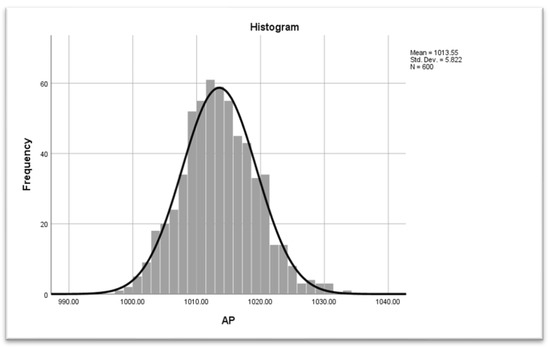
Figure 1.
Histogram of AP data.
Considering the first 600 observations as a population, 50 samples of size 5 each are drawn where the first 20 samples are taken assuming the IC process state, and the next 30 samples are drawn after introducing the shift in the process mean such that to imply the OOC process state. To monitor the process, the existing MA, EWMA, CUSUM, mixed EWMA-CUSUM, combined Shewhart-EWMA, combined Shewhart-CUSUM, and the EWMA-MA control charts are set up for a pre-fixed ARL0 = 370 and n = 5.
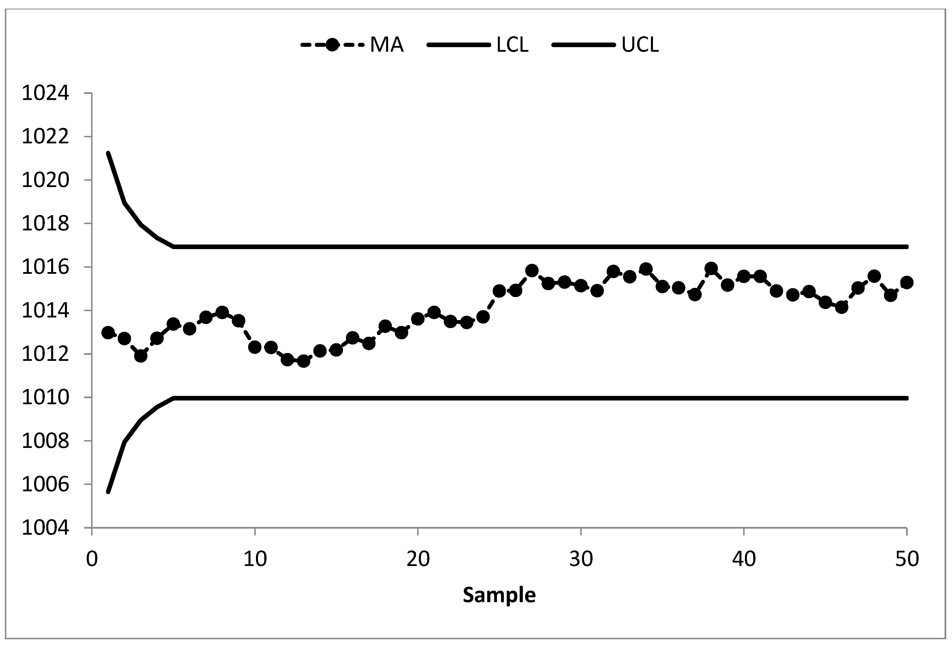
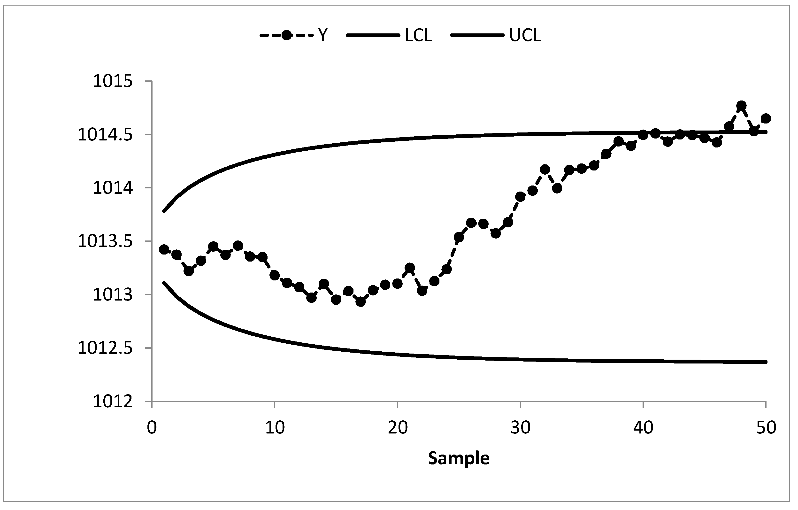
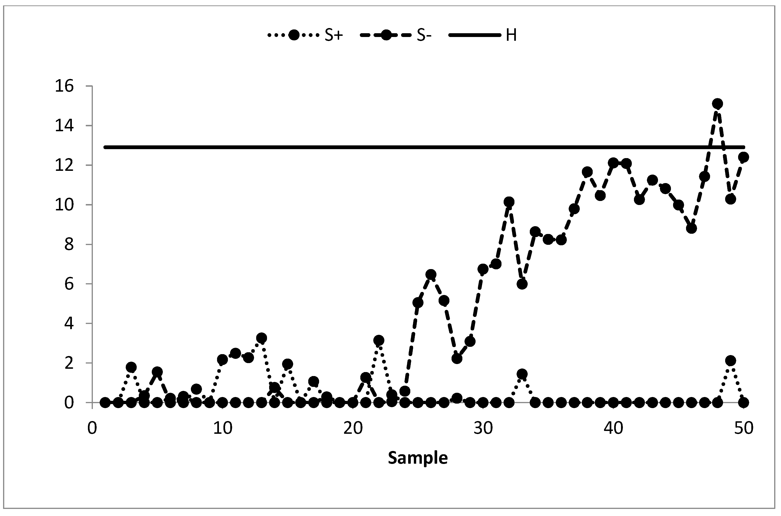
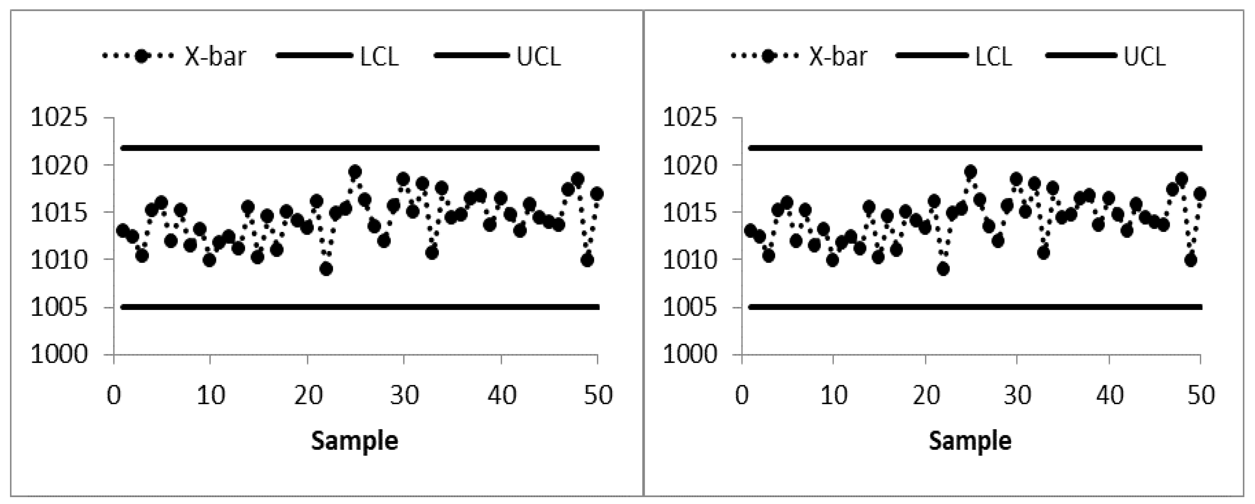
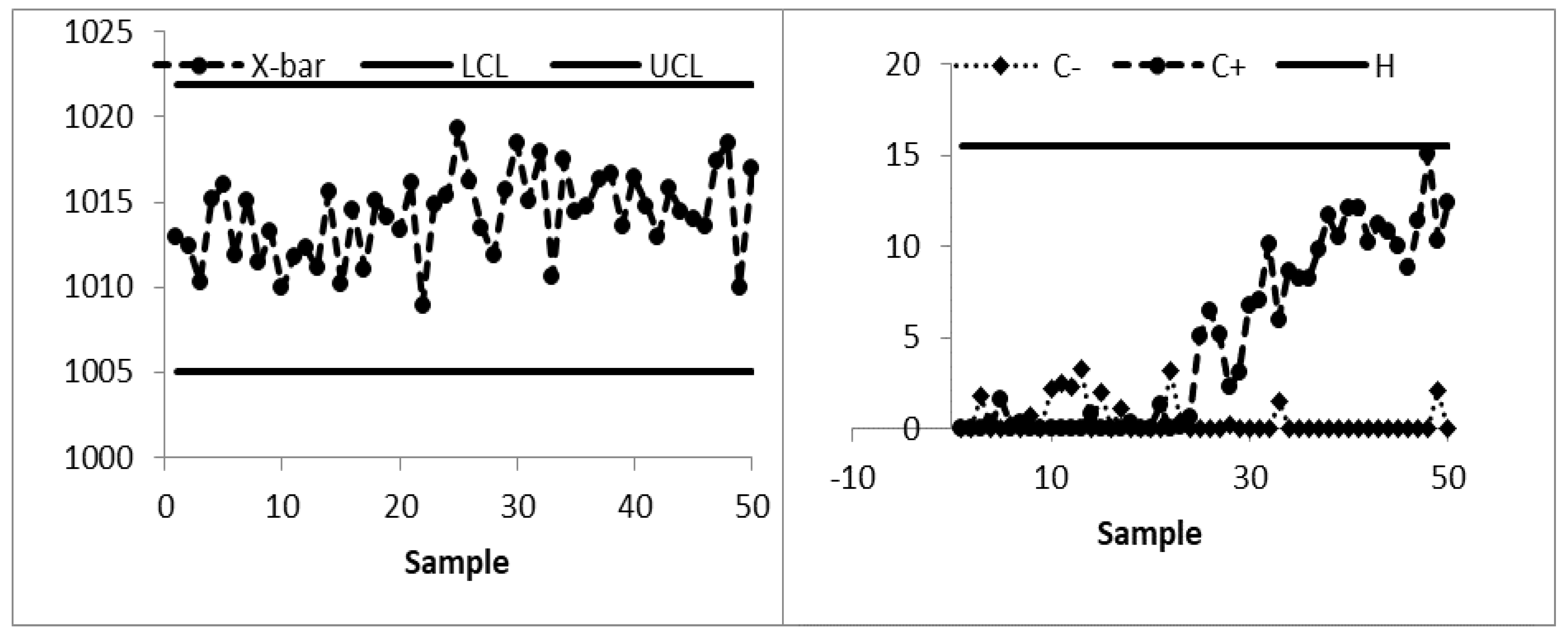
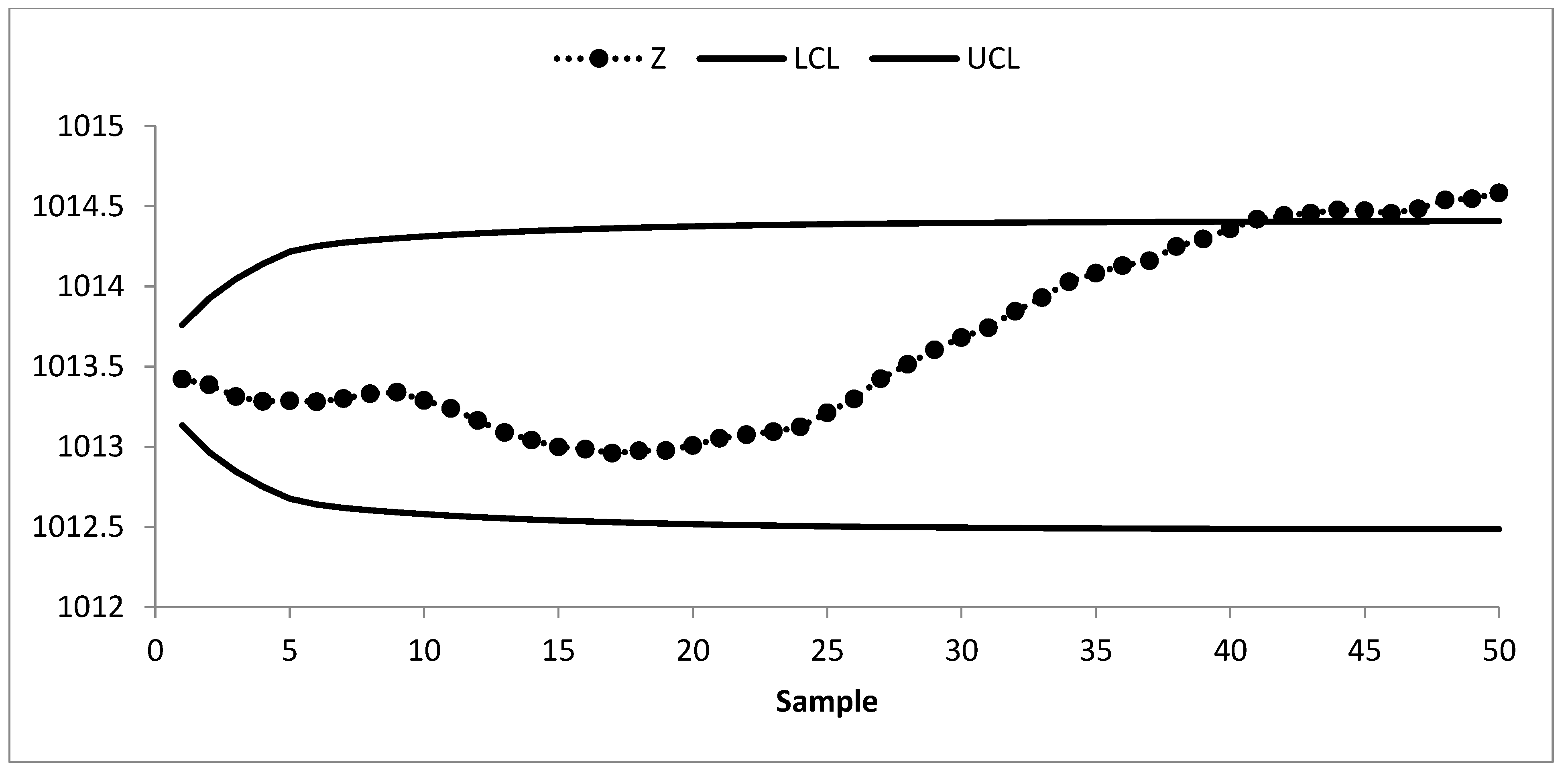
The existing MA control chart is constructed using w = 5 and displayed in Figure 2. It is observed that the MA chart fails to identify the shift in the process mean indicating the IC process state. The EWMA control chart is set up by using λ = 0.05 and shown in Figure 3. The EWMA control chart detects the shift at sample number 47. The existing CUSUM control chart is constructed using the design parameters k = 0.50 with h = 4.77 and shown in Figure 4. The CUSUM chart triggers an OOC signal at sample number 48. The existing mixed EWMA-CUSUM chart is set up by using the design parameters λ = 0.05, k = 0.50, and h = 45.54. Figure 5 depicts the mixed EWMA-CUSUM control chart that fails to detect the shift and declares the process to be IC. The combined Shewhart-EWMA control chart is set up by using L = 3.11, λ = 0.05, and K = 2.91. It detects the process shift at sample number 48 as shown in Figure 6. The combined Shewhart-CUSUM control chart is computed using L = 3.11, k = 0.5, and h = 5.75 and displayed in Figure 7. The chart fails to detect the shift in the process mean. Finally, the EWMA-MA control chart is set up with design parameters λ = 0.05, w = 5, and L = 2.311 as shown in Figure 8. It triggers an OOC signal at point 41 which is the 21st sample after the introduction of a shift in the process mean. These results clearly show that the EWMA-MA control chart has a superior mean shift detection ability as compared to other existing control charts, which further confirms the simulated results.
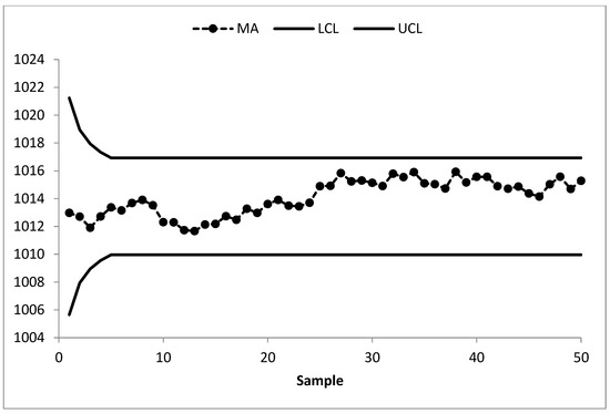
Figure 2.
MA control chart of AP data at w = 5 and ARL0 = 370.
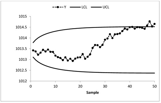
Figure 3.
EWMA control chart of AP data at λ = 0.05, L = 2.492, and ARL0 = 370.

Figure 4.
CUSUM control chart of AP data at k = 0.50, h = 4.77, and ARL0 = 370.
Figure 5.
Mixed EWMA-CUSUM control chart of AP data at λ = 0.05, k = 0.50, h = 45.54, and ARL0 = 370.
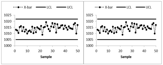
Figure 6.
Combined Shewhart-EWMA control chart of AP data for L = 3.11, λ = 0.05, and K = 2.91 at ARL0 = 370.
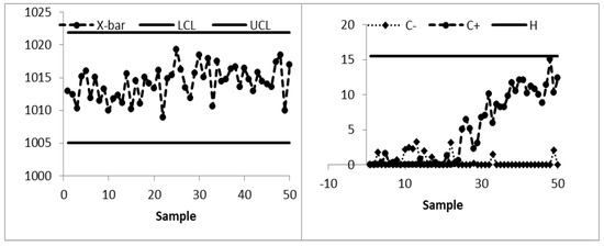
Figure 7.
Combined Shewhart-CUSUM control chart of AP data for L = 3.11, k = 0.5, and h = 5.75 at ARL0 = 370.
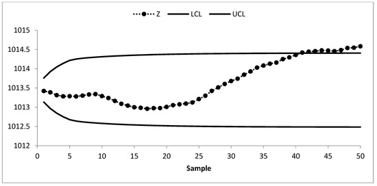
Figure 8.
Mixed EWMA-MA control chart of AP data at λ = 0.05, w = 5, L = 2.311 and ARL0 = 370.
6. Summary and Conclusions
In the SPC literature several mixed/combined control charting strategies were introduced to enhance the sensitivity of the control charts to quickly detect a range of shifts in the process parameters. Recently, Sukparungsee et al. [20] developed a mixed EWMA-MA control chart for quick detection of small to moderate shifts in the process mean. Their charting strategy assumed successive moving averages as independent and excluded the covariance terms from the variance expression of the EWMA-MA statistic. This approach is inappropriate as the MA terms are dependent and have at least one common term when their distance is less than the span w. Thus, their strategy may result in misleading decisions about the process state. In this study, the revised mixed EWMA-MA control chart is presented, and a comprehensive comparison of its performance is made with several competing combined control charting structures by using various run-length characteristics that were lacking in Sukparungsee et al. [20]. The comparison established the better shift detection ability of the revised mixed EWMA-MA control chart. Moreover, a robustness study is carried out to assess the effects of non-normality on the in-control run-length distribution of the EWMA-MA control chart. The results of the robustness study showed that the revised EWMA-MA control is somewhat resistant to non-normality, especially for smaller values of the smoothing parameter λ. Finally, to demonstrate the practicability of the EWMA-MA chart, an example from real-life data from a combined cycle power plant was used to monitor the ambient pressure that can affect the efficiency of gas turbine. The results further confirm the superiority of the EWMA-MA chart over the existing individual and combined charting schemes.
Author Contributions
Conceptualization, M.A.R., T.N. and K.I.; methodology, M.A.R. and K.I. validation, M.A., G.M.E. and S.H.B., formal analysis, M.A.R. and T.N. Writing—original draft, M.A.R., K.I., T.N., S.H.B. and G.M.E.; Writing—review & editing, M.A.R., T.N. and M.A. All authors have read and agreed to the published version of the manuscript.
Funding
This research is not funded by any organization.
Institutional Review Board Statement
Not Applicable.
Informed Consent Statement
Not Applicable.
Data Availability Statement
Not Applicable.
Conflicts of Interest
The authors declare no conflict of interest.
References
- Shewhart, W.A. Quality control charts. Bell Syst. Tech. J. 1926, 5, 593–603. [Google Scholar] [CrossRef]
- Page, E.S. Continuous inspection schemes. Biometrika 1954, 41, 100–115. [Google Scholar] [CrossRef]
- Roberts, S. Control chart tests based on geometric moving averages. Technometrics 1959, 1, 239–250. [Google Scholar] [CrossRef]
- Roberts, S. A comparison of some control chart procedures. Technometrics 1966, 8, 411–430. [Google Scholar] [CrossRef]
- Montgomery, D.C. Introduction to Statistical Quality Control, 8th ed.; John Wiley & Sons: Hoboken, NJ, USA, 2019. [Google Scholar]
- Lucas, J.M. Combined Shewhart-CUSUM quality control schemes. J. Qual. Technol. 1982, 14, 51–59. [Google Scholar] [CrossRef]
- Lucas, J.M.; Saccucci, M.S. Exponentially weighted moving average control schemes: Properties and enhancements. Technometrics 1990, 32, 1–12. [Google Scholar] [CrossRef]
- Shamma, S.E.; Shamma, A.K. Development and evaluation of control charts using double exponentially weighted moving averages. Int. J. Qual. Reliab. Manag. 1992, 9, 18–25. [Google Scholar] [CrossRef]
- Khoo, M.B.; Wong, V. A double moving average control chart. Commun. Stat.-Simul. C. 2008, 37, 1696–1708. [Google Scholar] [CrossRef]
- Haq, A. A new hybrid exponentially weighted moving average control chart for monitoring process mean. Qual. Reliab. Eng. Int. 2013, 29, 1015–1025. [Google Scholar] [CrossRef]
- Abbas, N.; Riaz, M.; Does, R.J. Mixed exponentially weighted moving average–cumulative sum charts for process monitoring. Qual. Reliab. Eng. Int. 2013, 29, 345–356. [Google Scholar] [CrossRef]
- Zaman, B.; Riaz, M.; Abbas, N.; Does, R.J. Mixed cumulative sum–exponentially weighted moving average control charts: An efficient way of monitoring process location. Qual. Reliab. Eng. Int. 2015, 31, 1407–1421. [Google Scholar] [CrossRef]
- Ali, R.; Haq, A. A mixed GWMA–CUSUM control chart for monitoring the process mean. Commun. Stat.—Theory Methods 2018, 47, 3779–3801. [Google Scholar] [CrossRef]
- Alevizakos, V.; Chatterjee, K.; Koukouvinos, C.; Lappa, A. A double moving average control chart: Discussion. Commun. Stat.-Simul. C. 2022, 51, 6043–6057. [Google Scholar] [CrossRef]
- Alevizakos, V.; Chatterjee, K.; Koukouvinos, C. The triple exponentially weighted moving average control chart. Qual. Technol. Quant. Manag 2021, 18, 326–354. [Google Scholar] [CrossRef]
- Rasheed, Z.; Zhang, H.; Arslan, M.; Zaman, B.; Anwar, M.S.; Abid, M.; Abbasi, S.A. An efficient robust nonparametric triple ewma wilcoxon signed-rank control chart for process location. Math. Probl. Eng. 2021, 2021, 1–28. [Google Scholar] [CrossRef]
- Engmann, G.M.; Han, D. Multichart Schemes for Detecting Changes in Disease Incidence. Comput. Math. Methods Med. 2020, 2020, 1–14. [Google Scholar] [CrossRef]
- Raza, M.A.; Aslam, M.; Farooq, M.; Sherwani, R.A.K.; Bhatti, S.H.; Ahmad, T. A new nonparametric composite exponentially weighted moving average sign control chart. Sci. Iran. 2022, 29, 290–302. [Google Scholar] [CrossRef]
- Han, D.; Tsung, F.; Hu, X.; Wang, K. CUSUM and EWMA multi-charts for detecting a range of mean shifts. Stat. Sin. 2007, 17, 1139–1164. [Google Scholar]
- Sukparungsee, S.; Areepong, Y.; Taboran, R. Exponentially weighted moving average-moving average charts for monitoring the process mean. PLoS ONE 2020, 15, e0228208. [Google Scholar] [CrossRef]
- Khan, N.; Aslam, M.; Jun, C.H. A EWMA control chart for exponential distributed quality based on moving average statistics. Qual. Reliab. Eng. Int. 2016, 32, 1179–1190. [Google Scholar]
- Han, D.; Tsung, F. A reference-free cuscore chart for dynamic mean change detection and a unified framework for charting performance comparison. J. Am. Stat. Assoc. 2006, 101, 368–386. [Google Scholar] [CrossRef]
- Raza, M.A.; Nawaz, T.; Aslam, M.; Bhatti, S.H.; Sherwani, R.A.K. A new nonparametric double exponentially weighted moving average control chart. Qual. Reliab. Eng. Int. 2020, 63, 68–87. [Google Scholar] [CrossRef]
- Qiu, P. Introduction to Statistical Process Control; CRC Press Chapman & Hall: Boca Raton, FL, USA, 2013. [Google Scholar]
- Cambron, P.; Masson, C.; Tahan, A.; Pelletier, F. Control chart monitoring of wind turbine generators using the statistical inertia of a wind farm average. Renew. Energ. 2018, 116, 88–98. [Google Scholar] [CrossRef]
- Benedetti, M.; Bonfà, F.; Introna, V.; Santolamazza, A.; Ubertini, S. Real time energy performance control for industrial compressed air systems: Methodology and applications. Energies 2019, 12, 3935. [Google Scholar] [CrossRef]
- Tüfekci, P. Prediction of full load electrical power output of a base load operated combined cycle power plant using machine learning methods. Int. J. Electr. Power Energy Syst. 2014, 60, 126–140. [Google Scholar] [CrossRef]


Disclaimer/Publisher’s Note: The statements, opinions and data contained in all publications are solely those of the individual author(s) and contributor(s) and not of MDPI and/or the editor(s). MDPI and/or the editor(s) disclaim responsibility for any injury to people or property resulting from any ideas, methods, instructions or products referred to in the content. |
© 2023 by the authors. Licensee MDPI, Basel, Switzerland. This article is an open access article distributed under the terms and conditions of the Creative Commons Attribution (CC BY) license (https://creativecommons.org/licenses/by/4.0/).