Abstract
Estimating wind energy at a specific wind site depends on how well the real wind data in that area can be represented using an appropriate distribution function. In fact, wind sites differ in the extent to which their wind data can be represented from one region to another, despite the widespread use of the Weibull function in representing the wind speed in various wind locations in the world. In this study, a new probability distribution model (normal PDF) was tested to implement wind speed at several wind locations in Jordan. The results show high compatibility between this model and the wind resources in Jordan. Therefore, this model was used to estimate the values of the wind energy and the extracted energy of wind turbines compared to those obtained by the Weibull PDF. Several artificial intelligence techniques were used (GA, BFOA, SA, and a neuro-fuzzy method) to estimate and predict the parameters of both the normal and Weibull PDFs that were reflected in conjunction with the actual observed data of wind probabilities. Afterward, the goodness of fit was decided with the aid of two performance indicators (RMSE and MAE). Surprisingly, in this study, the normal probability distribution function (PDF) outstripped the Weibull PDF, and interestingly, BFOA and SA were the most accurate methods. In the last stage, machine learning was used to classify and predict the error level between the actual probability and the estimated probability based on the trained and tested data of the PDF parameters. The proposed novel methodology aims to predict the most accurate parameters, as the subsequent energy calculation phases of wind depend on the proper selection of these parameters. Hence, 24 classifier algorithms were used in this study. The medium tree classifier shows the best performance from the accuracy and training time points of view, while the ensemble-boosted trees classifier shows poor performance regarding providing correct predictions.
1. Introduction
Long ago, it was understood that the continuous usage of conventional energy sources (fossil fuel) jeopardizes and threatens the stability of life. As a result, humanity has tried to find other inexhaustible energy resources to tackle the issues of the undesired impacts of the dominant energy sources (fossil fuel). Renewable energy sources were the best alternative, which became grist, an integral part, and the interesting core of the energy sector due to their immense valuable features [1]. Furthermore, the lack of conventional energy resources boosts the harnessing of clean energy sources [2]. Inasmuch, the development of lifestyle is associated with energy demand. As such, the larger the energy demand in a certain area, the most sophisticated the area [3,4,5,6,7].
Wide choices of renewable energy are available, such as solar, the internal heat of the earth, wind, tidal, and biomass energy [8]. Wind energy has played a prominent, astounding, and marvelous role in contributing to the depreciation of carbon dioxide [9], which has encouraged some countries to invest in wind energy [10]. The key to wind energy is its kinetic energy; the energy that can be harvested by wind turbines fundamentally depends on the average wind speed. The most effective areas to install a wind farm are those located beside coasts, on the edge of water bodies, and in open terrain [11]. Figure 1 shows the worldwide distribution of wind energy [12].
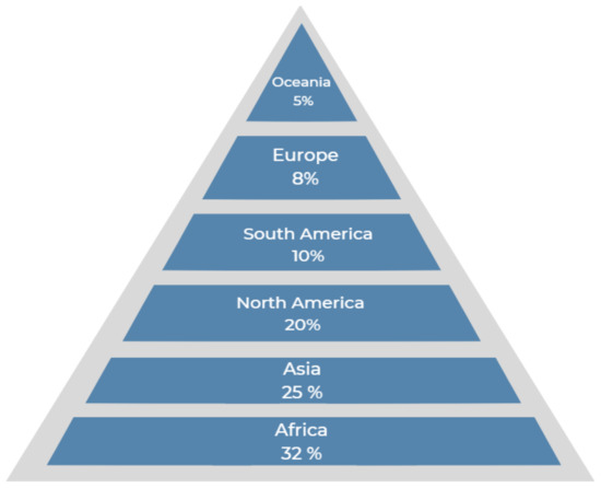
Figure 1.
The worldwide distribution of wind energy.
Wind energy is defined as an inherently unfixed energy source, which varies rapidly over time [13]. It is dramatically growing and ubiquitous since this type of renewable energy has several strong points which make it outstrip fossil fuel; for example, it can meet the massive demand for energy and minimize the pollution resulting from fossil fuel usage up to a certain limit. Consequently, wind energy is deemed a green energy technology [14]. In addition, wind energy projects contribute to enhancing the situation of the environment, economy, and society [15].
Wind turbines can be installed on ranches or farms, which improves the economic situation, as mentioned before, chiefly in rural regions where the best sites for wind are found. These turbines do not generate any atmospheric emissions that are responsible for greenhouse gases and acid rain, which makes wind energy eco-friendly, as mentioned before [16,17].
Among the types of renewable energy, the consumption of wind energy is the largest category in most countries [18]. For illustration, it constitutes about more than 20% of the total renewable energy, and this percentage is increasing continuously [19,20]. The global capacity of wind was about 336.327 GW in June 2014. However, 17.613 GW of this was installed in the first half of the same year [21]. In particular, Jordan is considered a country where the wind is available in abundance. The attention to wind energy began in Jordan in 1979, and these days, Jordan has decided to provide 20% of the required energy from wind and solar energy [22]. Several wind projects exist, such as the Tafilah wind project, which delivers almost 132 MW of electricity to the national grid; meanwhile, some other wind projects deliver about 25 MW of electricity [23,24,25,26,27,28]. Moreover, Jordan has been deemed as one of the Arab countries which contributes to the spread of the culture of renewable energy exploitation; notably, by the end of 2021, the installed renewable energy projects will contribute to electricity generation by a percentage of 20.1% generally and 15.3% by the wind, as clarified in Figure 2. Accordingly, the awareness of wind energy has increased abruptly and attracted attention, which is the reason for installing two new wind farms in 2021 with a capacity of 51.75MW each [29]. Figure 3 represents the MW production from wind during the period from 2010 to 2021 in Jordan [30].
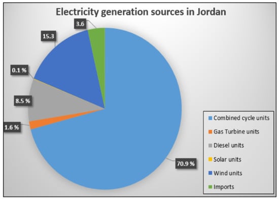
Figure 2.
Electricity generation sources in Jordan.
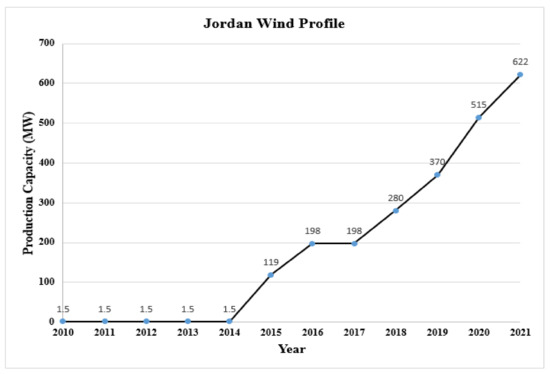
Figure 3.
Wind Profile of Jordan.
The output of wind power depends mainly on the speed of the wind. Hence, it is irrefutable that evaluating the distribution of wind speed is considered the starting point for wind energy potential assessment purposes [31]. Usually, the distribution of wind speed is estimated and described by several probability distribution functions (PDFs) [32], especially by the Weibull PDF, since the estimated outcomes are close to the actual observed wind speed. In addition, the Rayleigh PDF, which is a special case of the previously mentioned PDF (Weibull), is used in some studies, and sometimes, it provides a better fitting [33]. Therefore, it can be understood that no particular PDF can fit the distribution of wind speed in all sites meticulously, bearing in mind that the estimation of wind speed is not simple because of the stochastic nature of the wind source and frictional and roughness effects [34,35,36].
Several recent studies stated that estimating the wind turbines’ P-V curve is required in the preliminary assessment of the wind turbines’ energy yield [37]. However, different methods have been proposed to make an initial assessment and estimation of wind speed with an uneven degree of resolution and accuracy [38]. Kevin et al. proposed a technique in [39] that endorsed a study conducted by Al-Mhairat et al. in [1], showed that gamma PDF outperforms the other PDFs in wind assessment. This study was performed in Kenya and aimed to specify the optimal parameters of the selected distribution functions, which were Weibull, log-normal, and gamma. The process of this study was conducted by estimating the PDFs’ parameters by using a numerical approach, that is, the maximum likelihood method (MLM).
Consequently, Rejhana [40] decided to use two methods to estimate the parameters of the Weibull PDF and the wind power density, which are the MLM and the energy pattern factor methods. The outcomes showed that the wind energy that is available in Sarajevo is not enough to meet the required energy for that region.
Similarly, Boro et al. in [41] used the MLM in order to compare the accuracy of various PDFs, including the inverse Gaussian, gamma, Rayleigh, hybrid Weibull, and Weibull PDFs. Some statistical tools were used as indicators, such as the coefficient of determination (R2) and root-mean-square error (RMSE). The results stated that there is not only one PDF that fits the whole region worldwide, such that in some sites, such as Ouahigouya, Dédougou, and Ouaga, the Weibull PDF was the most suitable one, while in other sites, such as Gaoua, Dori, and Boromo, it was found that the inverse Gaussian PDF was the most suitable one.
Saeed et al. in [42] aimed to improve the performance of the Weibull PDF by using artificial intelligence optimization techniques (AIOP) to obtain the highest possible precision from the Weibull PDF. This study was conducted in thirteen different sites in Pakistan and tried to provide an alternative method for the estimation of parameters for the Weibull PDF. Further, the convergence was enhanced in this study by three AIOTs. The results showed that the proposed method for estimating the parameters of the Weibull PDF outperforms the common Weibull PDF.
However, some studies used both Weibull and Rayleigh PDFs in wind speed estimation. The reason for being the two most common PDFs is their accuracy in predicting and describing wind speed. For instance, Bidaoui et al. in [43] evaluated the potential of wind energy by using stochastic models of Rayleigh and Weibull PDFs of five locations in Northern Morocco. Some indicators were utilized, such as the mean bias error (MBE), RMSE, Chi-square error (χ²), and R2. The outcomes of this study indicated that the accuracy of the Weibull PDF is higher than the Rayleigh PDF.
Abeysirigunawardena et al. in [44] claimed in their study that the maximum likelihood estimation (MLE) approach is the most commonly used in wind estimation. This method can mix various information with the parameters of the model. Moreover, the results showed that approximate standard errors for the estimated parameters may be shaped automatically.
Baloch et al. stated in [45] that a sensitivity analysis is usually conducted in order to test the effectiveness of varying the parameters. Several research studies were conducted to study the effect of distribution function parameter variations on the energy of both wind regimes and wind turbines [46,47,48]. However, the goal of proposing new approaches is to be able to select accurate parameters for each PDF such that the estimated probability becomes very close to the actual one. Accordingly, the subsequent applications based on these parameters will become more reliable. The previously mentioned recent studies are summarized in Table 1.

Table 1.
Summary for the previous studies in the same field of research.
The importance of the PDF is summarized by being able to make a description and prediction for the probability of a certain event. Each PDF carries its own parameters, and the right selection of these parameters will be reflected in a proper application. The normal PDF depicts one of the most common PDFs that is commonly used in estimating probability [49]. This PDF is represented by two main parameters, µ, which is the mean value that describes the central tendency, and σ, which is the standard deviation that describes how the probability values are dispersed around the central point. [50]. Moreover, the Weibull PDF is also considered an accurate PDF that is used in wind variation estimation. This PDF is represented by two main parameters, K, which is the shape factor, and C, which is the scaling factor [51].
The main contribution of this study compared to other studies in the same field of research can be summarized by the following:
- This study estimates the wind energy and extracted energy of a wind turbine using a new distribution function (normal) that has not regularly been used in the literature.
- The estimation method of this study is performed using several artificial intelligence methods with the aid of machine learning classifiers that have not previously been used in other studies.
However, wind speed can be measured by several apparatuses, such as the cup anemometer, which is represented in Figure 4a [52]; this technology responds promptly to wind movement, but this device cannot stop immediately once the wind stops [53]. Moreover, another technology that is used in wind speed measuring is the propeller anemometer, which is represented in Figure 4b [52], while sonic anemometers are used for both wind speed and direction measurement, which is represented in Figure 4c [54].
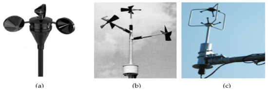
Figure 4.
Technologies that are used in wind speed measurement. (a) Cup anemometer; (b) propeller anemometers; and (c) sonic anemometer.
2. Methodology
Innumerable choices for studying the extractable energy from wind are available nowadays; the chosen method strongly depends on statistical science. The general methodology adopted to accomplish this study is clarified and depicted in Figure 5.
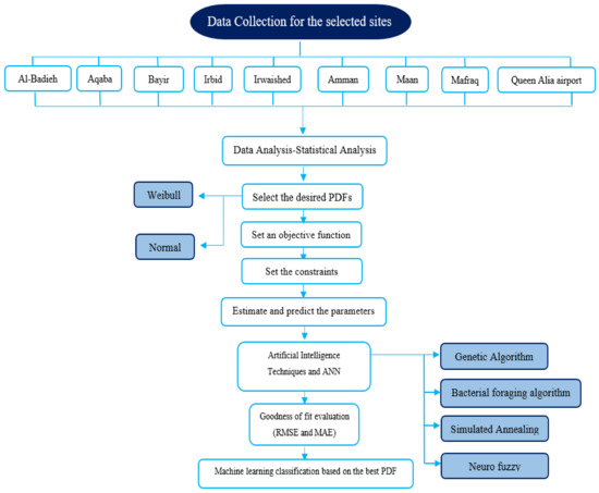
Figure 5.
Flowchart steps of the intended study.
2.1. Data Collection for the Whole Site
An abundant number of marvelous research were conducted to achieve the goal of developing some reliable and sophisticated methods for wind forecasting. Each method has a tolerance percentage and does not match the actual wind measurements strictly.
In other words, the only essence disparity that differs vividly from one strategy to another is the uneven level of rigor. However, these methods are clarified in Figure 6 [55].
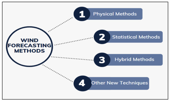
Figure 6.
Forecasting methods for wind measurements.
The physical approaches use several types of physical information, including, to name a few, wind conditions, especially at the turbine hub’s height, the power curve of the wind turbine, data from the meteorological departments, and the weather conditions, by and large. Regardless, these physical data are borne in mind to estimate wind readings.
In juxtaposition, statistical methods can forecast either wind speed power probability or wind speed/power value. Both are commonly obtained based on statistical analyses of time series, which depend on past observed wind data.
The third astounding method is the hybrid approach, which is a combination of several methods, such as physical methods in conjunction with statistical methods. Finally, the fourth method is other new techniques such as entropy-based training, ensemble predictions, wavelet transform, fuzzy logic, and spatial correlation.
In this paper, the daily wind speed data have been collected from RETScreen software for nine sites in Jordan, which are clarified in Table 2 with their corresponding details. The raw data period was for one complete year, starting from 1 October 2021 and going to 30 September 2022. All of these data were recorded at a 10 m height.
Table 2.
The latitude, longitude, and elevation of the proposed sites [56].
2.2. Data Analysis and Statistical Analysis
Currently, modern turbines have a hub height of around 100 m, while the wind data were measured at 10 m, as mentioned afore. Therefore, the first step in wind data analysis is carried out by making a conversion for the obtained wind speed at 10 m into corresponding data at 100 m. The reflected wind speed at 100 m is obtained by applying Equation (1) [57].
where V2 represents the desired wind speed at the extrapolated height, V1 represents the wind speed at the reference level, h2 represents the desired height, and h1 represents the reference height. Finally, the symbol represents the wind shear exponent (WSE) that discerns and describes the terrain situation of the site. Table 3 clarifies several scenarios for the factor of the proposed sites. The following subsections clarify how the corrected wind speed was analyzed statistically.
Table 3.
Details regarding the WSE [58].
2.2.1. Selecting the Candidate PDFs
The current trend is to use the probability density function (PDF) approach to assess wind energy resources. The Weibull approach is the most ubiquitous PDF that has been used in most recent studies in wind assessment. This research sheds light on another PDF, the well-known normal PDF, to assess wind in several sites in Jordan. The mathematical representations for the proposed PDFs are clarified in the following points [59].
- (A).
- Weibull
As stated before, the wind speed probability for a certain region is often expressed and represented by the Weibull PDF. Based on the following mathematical representation, it can be observed that this PDF has two main parameters, which are the shape and the scale factor.
- (B).
- Normal
The second proposed PDF in this paper is the normal PDF, which is also known as the Gaussian distribution. This distribution function is called the Gaussian distribution by physicists and the bell curve by social scientists [60]. The following mathematical formula shows the PDF for the normal function:
where and are the standard deviation and the mean wind speed.
Analyses of wind speed can be made by the PDFs. Thus, the more precise the selected parameters, the more accurate and more satisfactory the outcomes. In other words, the estimation of the parameters is the springboard, and it is considered a critical phase that plays an essential role in achieving the desired and accurate outcomes. The performance of the PDFs relies on several factors, such as the number of data, the evaluation criteria, and the period of data measuring.
2.2.2. Set an Objective Function
A power curve of a wind turbine is defined as a visual representation of the generated electrical output power for each corresponding wind speed. The lofty goal of capturing and exploiting the wind is to produce electrical power. Therefore, it is necessary to link these two parameters (electrical power and intermittent wind speed) in order to comprehend how they affect each other. The power curve of wind turbines that depicts the relationship between the electrical power output and the wind speed is known as the P-V curve, and each wind turbine model has its own P-V curve. This curve is essential for many purposes, chiefly for project conducting and planning, monitoring the turbines, and detecting the likelihood of the maloperation of turbines [61].
Producing electrical power from wind energy at the sites under investigation relies on immense factors, including the mean wind speed and wind turbine speed characteristics, which involve the cut-in speed, rated speed, and cut-out speed. The available energy in the wind varies with the variation in wind speed. Hence, understanding the P-V characteristics of wind is essential in wind assessment. Figure 7 clarifies a typical representation of the ideal P-V curve.
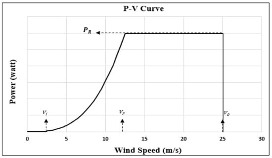
Figure 7.
P-V curve of an ideal wind turbine.
It is apparent in Figure 7 that, in the region before the cut-in speed, the output power from the wind turbine is zero since the cut-in speed is quite low and cannot produce enough power to overbear the friction of the wind turbine. However, even if the friction of the wind turbine has been overcome and a rotation of the generator is observed, the corresponding generated electrical power may be slight and not sufficient to offset the required power by the generator field windings. Per contra, once the wind speed increases above the cut-in speed, the resultant output power rapidly increases until it reaches a critical point where the output power flattens out. At this point, the turbine is reaching its upper limit of generation, which is known as the rated output power. After a certain threshold value, which is around 25 m/s, the next wind speed is known as the cut-out speed, where the turbine initiates shut-down mode for protection purposes since the blades are at risk because of the large applied force. Hence, based on the previous clarification, the symbols refer to cut-in speed, rated wind speed, cut-out speed, and rated power, respectively. However, the most important parameter of this curve is , which describes the nonlinear region.
The enclave region between the cut-in speed and the rated wind speed (nonlinear region) can be represented using several mathematical formulas. Therefore, the output power from a wind turbine can be determined depending on the interval of wind speed, as illustrated below [62]:
In this research, four representations of Q(v) have been examined, which are [63]:
In this paper, the objective function is to maximize the energy captured by wind by the proper selection of the proposed PDFs’ parameters as illustrated in the following equations [64]:
Subject to:
where:
ETotal: Total energy that can be generated by the wind turbine ();
: The overall loss percentage of the turbine;
T: Time period in an hour;
Eir: Generated energy by the wind turbine in the region between the cut-in speed and rated speed in .
Ero: Generated energy by the wind turbine in the region from the rated speed to the cut-out speed in .
PO: The probability based on the observations (real data from RETScreen);
PD: The probability based on the proposed PDFs.
In general, the energy that is available from wind resources can be determined based on the following expression:
where:
The available energy in the regime;
The wind power density;
The used PDF;
The effective area of the disk;
The air density;
The velocity of the wind.
The attention in this research goes to tracking the maximum energy by varying the two parameters of the normal and Weibull PDFs such that the estimated probabilities must be close to the observed probabilities for each wind speed class.
2.2.3. Estimating and Predicting the Parameters by Artificial Intelligence Techniques in Conjunction with Neural Fuzzy Methods
In the design stage of any project implementation, optimization is an essential tool by which the performance of the overall system can be enhanced effectively. Furthermore, this tool is used in the whole field and is not limited to only one field due to the diversity of the dilemma nowadays. The intriguing ideas of the optimization algorithms were put forth depending on the behavior of things around us.
The concentration of this research is oriented toward estimating the parameters of the various distribution functions by optimization algorithms. Nowadays, artificial intelligence (AI) has become a trend due to its features. This technique programs the machine to be capable of performing complex tasks. Further, it works in various fields, which makes it popular these days [65].
In this study, three distinct algorithms are employed to estimate the parameters of the proposed PDFs. The first one is the genetic algorithm (GA), the second one is the bacterial foraging optimization algorithm (BFOA), and the third one is the simulated annealing (SA) algorithm. It is no wonder that artificial intelligence (AI) techniques are more recommended than numerical approaches due to their high level of accuracy and flexibility.
In this paper, the initial population of each parameter started from 0 to 100 for each PDF, with a step of 0.05 for each iteration. The goal of the AI was to find the best parameters that made the estimated wind speed as close as possible to the actual wind speed. Thus, the stopping criteria were based on finding the most accurate parameters by evaluating the holistic possibilities of the initial population.
- (A).
- Genetic Algorithm
The GA mimics the biological evolution natural process by selecting fit individuals for reproduction. It works with specific population sizes (individuals) that are evolving with time. The principle of this algorithm is inspired by human beings based on the three main operators: selection, crossover, and mutation. Figure 7 shows the implementation steps of GA based on [66].
Based on Figure 8, the principle of this algorithm can be simply explained as follows: the population of a certain number of chromosomes is generated randomly. The next step is to find the corresponding fitness value of each chromosome. Afterward, a single-point crossover is applied for the two chromosomes (two inputs of the optimization problem) to generate offspring. The applied crossover in this thesis is the partially matched crossover (PMX) method since it is the most commonly used crossover. The next step is to apply the mutation operation to the obtained offspring to generate a new population. Thereafter, the previous process (selection, crossover, and mutation) is applied again until a new population is obtained [67].
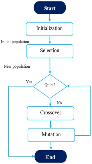
Figure 8.
Flowchart of GA.
- (B).
- Bacterial Foraging Optimization Algorithm
BFOA is considered an optimization approach that was developed depending on the base of Escherichia Coli (E. Coil) bacteria’s foraging strategy. These bacteria live inside the human gut. The term “foraging” refers to the animals’ behavior for ingesting, handling, or locating their food. In general, E. Coil bacteria have flagella, which enable the bacteria to rotate or move in a locomotion manner. For clarification, with the aid of the flagella, the bacteria may move in the same direction or change its orientation. The ultimate two goals of this bacteria are to find a place with a high level of nutrients and mitigate the noxious areas by moving in a certain motion. Hence, as a summary, when the bacteria reach a place with a higher level of nutrients compared with the previous place, the movement is described as “swimming” or “running”. Otherwise, it will tumble. Figure 9a,b clarifies the previous discussion. In Figure 9a, the bacteria move from location L1 into location L2 since the nutrient level in L2 is higher than in L1. It can be observed that the bacteria move forward within the same path, “swim”. Similarly, the bacteria move from L2 into L3, which indicates that L3 has more nutrient levels compared with L2. This process is repeated until the phase-out of the bacteria’s life.
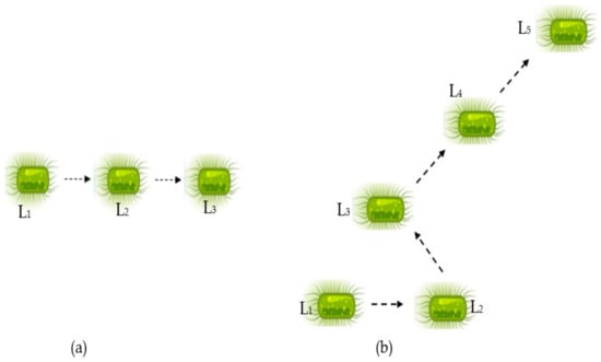
Figure 9.
Bacteria movement based on the nutrient level in each location where (a) represents “swimming” case, and (b) represents “swimming and tumbling” case.
The second mentioned case is clarified in Figure 9b. This case may include swimming beside tumbling. In this case, the initial location is L1; the bacteria try to find another location, and the nutrient levels of the two locations are compared. If the nutrient level of the new location is higher, the bacteria will go toward (swimming) this area; otherwise, it will search for another location with a higher nutrient level by changing its trajectory (tumbling). Since the nutrient level at L2 is lower than that of L1, the bacteria will not continue moving with the same path but will move in another path until reaching L3, where the nutrient level is higher in comparison with the previous location. Another test for nutrient level will be conducted; if at L3 the nutrient level is lower than that of L2, the bacteria will tumble and move into another location, L4. If the nutrient level at L4 is higher than that of L3, the bacteria will swim in the same path of the previous movement until a new location, L5, is reached [68]. The flowchart of this algorithm is clarified in Figure 10, where Nd refers to the number of elimination-dispersal events, Nre refers to the number of reproduction steps, and Nc refers to the number of chemotactic steps [69].
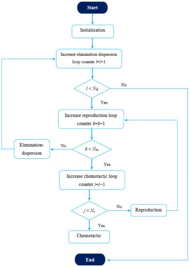
Figure 10.
Flowchart of BFOA.
- (C).
- Simulated Annealing Algorithm
The idea of the simulated annealing (SA) algorithm mimics the metal reshaping process, where a heated metal is reshaped from one structure to another after being cold. An initial solution is set randomly and then based on this procedure, which is clarified in Figure 11 [70]. The control parameter in this algorithm is the temperature, which controls the number of iterations of the process [71]. In the end, the best fit which meets the objective function will be selected. Based on Figure 11, it can be noticed that SA has a sequence of moving from the initial solution toward the next solution, where in some cases, the worst solution may be accepted based on a probability factor.
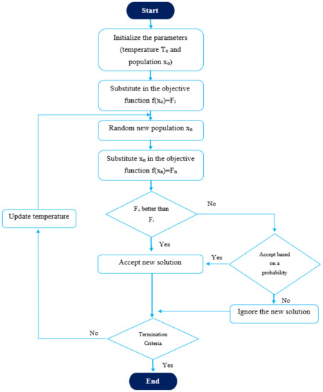
Figure 11.
Flowchart of SA.
- (D).
- Adaptive Neural Fuzzy Inference System (ANFIS)
Fuzzy logic is a worthwhile tool in conducting complex tasks, especially when it is difficult to obtain a mathematical model. In addition, fuzzy logic may be used in prediction problems for quality amelioration purposes. In contrast, neural networks (NNs) are networks that can link the input with the output data in a certain manner, where each input is assigned a certain value of weight. Subsequently, the output is determined based on the assigned weights [72].
However, in this paper, a combination of these two techniques is used, where ANFIS is classified as a hybrid AI model that coalesces and combines the intrinsic features of fuzzy logic in the parallel processing of a NN [72]. The architecture appears from the tool itself for the proposed problem, which has two inputs and a single output. The flowchart of ANFIS is presented in Figure 12 and Figure 13 [73].
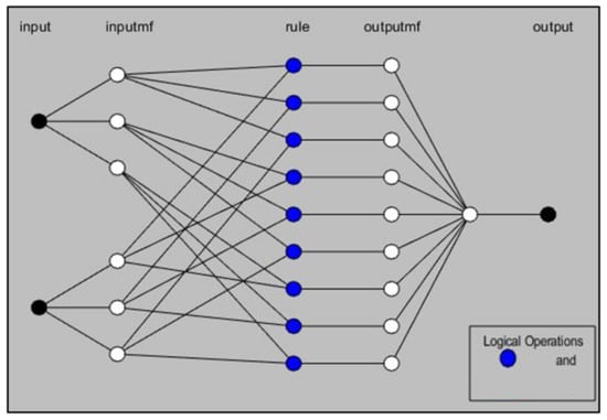
Figure 12.
Architecture of ANFIS.
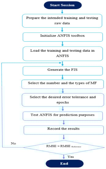
Figure 13.
Flowchart of ANFIS.
ANFIS became a technique that can be used for predicting purposes, as it can make an input-output mapping and accordingly design an input-output prediction by the hybrid learning process. In general, ANFIS is commonly used to simulate nonlinear systems providing intrinsic and reliable outcomes [74].
2.2.4. Selecting the Most Accurate Approach Based on the Indicators (RMSE and MAE)
Estimating the parameters of the proposed PDFs is a non-trivial task, and the most challenging task is to opt for and decide which PDF model is the best. Based on the previously mentioned two methods of selecting the parameters (either by artificial intelligence techniques or by prediction), once the corresponding parameters of each PDF are selected, the next step is assigned to choose the most precise PDF. This can be accomplished with the aid of some goodness-of-fit (GOF) indicators, such as RMSE and MAE. Incontrovertibly, the lower the fitness value, the better the proposed model fit. Each proposed PDF is a candidate to be accepted if its parameters achieve a fitness value that is relatively small.
Several options for GOF tests are offered and available nowadays; in this study, RMSE and MAE are the proposed indicators since these two indicators are the most frequently employed in evaluating accuracy. The mathematical formulas for these indicators are illustrated in the following points [75].
- (A).
- RMSE:
The root-mean-square error (RMSE) between X datasets (the observed probability) and Y datasets (the estimated probability) is defined as a measurement of the difference between their values and can be expressed as:
This indicator is commonly used to assess how good the predicted probability is over the observed probability, where the smaller value of RMSE is, the better the accuracy of the proposed model, indicating that the selected parameters achieve the best results.
- (B).
- Mean Absolute Error (MAE)
This test determines the absolute error between the observed value and the corresponding estimated value. This performance indicator looks similar to the RMSE since the lower the MAE, the better the outcomes obtained are. Its mathematical formula is represented below:
2.2.5. Machine Learning Classification and Prediction Based on the Best PDF
Machine learning (ML) is a description of a computer that has been programmed and trained based on a certain data pattern, thus becoming able to predict the situation for newly inserted data. This term (ML) is divided into two major categories: classification (supervised learning) and clustering (unsupervised learning). In classification, two phases are required: the training phase and the testing phase. In the training phase, the inserted data should be divided into a certain number of categories, where each category carries a particular percentage from the overall data that have the same classification. Commonly, the first columns in the intended trained data represent the input(s), while the last column represents how each input(s) has been classified. Within the same phase and based on several built-in classifier algorithms, the machine will be able to understand and learn the data. Accordingly, by generating a learning model while in the data testing phase, the data is classified based on the generated trained model in addition to the classifier model.
On the other hand, in clustering, the input data are grouped based on their similarities without any trained model. The purpose of using ML in this study is to be able to predict the difference (error) between the actual observed wind speed data and the estimated wind speed for the best PDF, which will be decided based on the performance indicators, as mentioned before. Here, a small error indicates that the selected parameters are good, while a medium error indicates that the selected parameters are not good enough, and finally, a Large error indicates that the selected parameters achieve a large difference between the observed and the estimated value.
In this paper, 24 classification algorithms have been used to run the data. These algorithms have been summarized in the last section of this paper. The significance of using ML in this study came from the necessity of the more precise prediction of the parameters since the remaining phases of energy estimation depend on the selected parameters.
3. Results and Discussion
The two parameters of the normal PDF, μ and σ, were selected intelligently by GA, BFOA, SA, and the neuro-fuzzy method. The corresponding energy regime in Kwh/year was determined accordingly based on each method for all sites, as clarified in Table 4. These parameters are reflected concurrently with the observed actual data of wind speed for all sites, as represented in Figure 14.
Table 4.
Outcomes for the normal PDF parameters by GA, BFOA, SA, and ANFIS along with the energy regime per year.
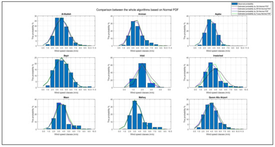
Figure 14.
Outcomes based on Normal PDF.
Similarly, the parameters of the Weibull PDF, K and C, were assigned by the same approaches of GA, BFOA, SA, and the neuro-fuzzy method. The corresponding energy regime in Kwh/year has been determined accordingly based on each method for all sites, as clarified in Table 5. These parameters are reflected in conjunction with the observed actual data of wind speed for all sites, as represented in Figure 15.
Table 5.
Outcomes for the Weibull PDF parameters by GA, BFOA, SA, and ANFIS along with the energy regime per year.
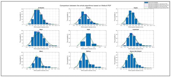
Figure 15.
Outcomes based on Weibull PDF.
In the end, the extractable energy from wind has been determined based on the four listed P-V models for both the normal and Weibull PDFs. The outcomes are summarized in Table 6 and Table 7, respectively, assuming the same wind turbine brand parameters for a fair comparison.
Table 6.
Extractable energy (MWh per year) based on Normal PDF.
Table 7.
Extractable energy (MWh per year) based on Weibull PDF.
3.1. Assessment of the Proposed Approaches
An assessment of the proposed approaches was carried out based on the GOF by two performance indicators (RMSE, MAE), as clarified in Table 8, to ascertain the accuracy of the selected parameters. The goal of this step was to rank the selectivity level of each approach depending on the minimal difference (error) between the observed data and the foreshadowed data. Hence, based on Table 8, it can be perceived that BFOA and SA are the most accurate and predominant approaches in selecting the parameters in both the normal and Weibull PDFs, with a slight ignorable difference between them compared with their counterparts. In addition, based on the same table, it can be noticed that the normal PDF gives more accurate and precise estimated outcomes compared with the Weibull PDF. Therefore, the classification of classes was conducted based on the normal PDF. Accordingly, based on the outcomes that were obtained from this study, the worthiest regions in Jordan that are rich in wind resources, headed by Bayir and wrapped up by Irbid, are arranged in Figure 16 based on the BFOA and SA algorithms.
Table 8.
Comparison between normal and Weibull PDFs based on several performance indicators for the four methods of parameter selection.
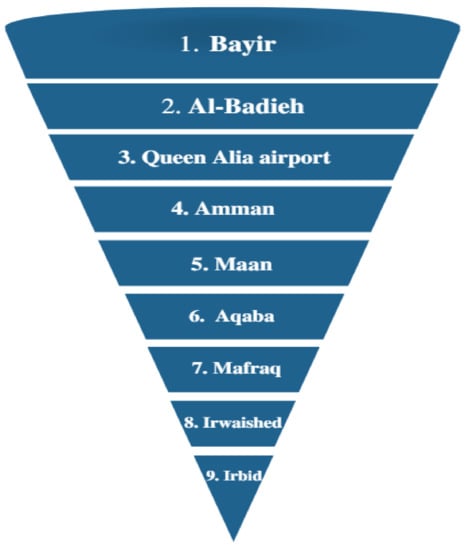
Figure 16.
The ranked sites in Jordan based on the availability of wind.
The bottom line of Table 8 is to emphasize that the Weibull PDF is not always the most accurate PDF but rather the opposite in this study, as it was found that the normal PDF overwhelmed the Weibull PDF.
3.2. Machine Learning Classification Outcomes
Several studies used ML in several fields, for instance, [76], in the diagnosis of the crime rate against women by using k-fold cross-validation. In [77], ML was used to conduct the sensitivity analysis of k-fold cross-validation, especially in error prediction and estimation. Another study conducted by [78] stated that ML is an effective and powerful tool, notably when massive amounts of data are collected.
In this study, a novel approach is proposed to classify and predict wind estimation by a MATLAB environment-classification learner application based on the datasets that were gathered from RETScreen, analyzed by the SPSS environment, and finally tested by AI codes. Hence, a huge dataset has been investigated to evaluate the performance of the normal PDF, where the nominated approaches try to find the best parameters of µ and σ that attain the least difference (error) between the observed and estimated probabilities for each site. The sample size comprises 3000 species for each candidate site; these 3000 were divided into three main categories. Thus, three distinct classifications were assigned, low error, medium error, and large error, based on each case of µ and σ and the resultant error. Each classifier has its accuracy percentage, cost misclassification, and training time. Therefore, the trade-off between them was based on the accuracy percentage in the first level, then on the training time if several classifiers gave the same accuracy percentage.
The validation process of the inserted data can be made by three options, cross-validation (x-validation), holdout validation, and no validation. Each approach has its features, where the cross-validation approach mitigates the situation of overfitting by dividing the whole raw data into a certain number of folds, while holdout validation is recommended to be used in large data sets. Finally, with no validation option, there is no protection against overfitting. In this study, the k-fold cross-validation method was used to validate the behavior of the generated learned model, where a certain number of folds equal to 5 was set. In other words, the inserted data was divided into five groups; one group was used for testing in the testing phase, while the remaining four groups were used for learning purposes in the training phase, as clarified in Figure 17. Generally, the k-fold cross-validation method has five main steps to be implemented, which are summarized in Figure 18. The principle of k-fold cross-validation can be explained by splitting the data into k groups, where each group carries an equal data sample weight; afterward, each group will be used as a test group for one time and as a training group for k-1 times. This validation approach is very common since it is easy to understand [76].
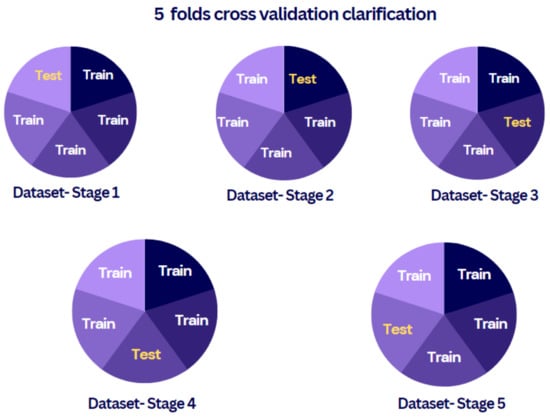
Figure 17.
Five-fold cross-validation demonstration.
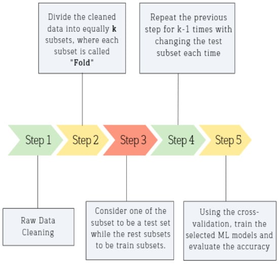
Figure 18.
Steps of applying K-fold validation.
In general, the corresponding performance of any classifier is represented by the confusion matrix from an accuracy point of view, as clarified in Figure 19 in terms of true-positive rate (TPR) and false-positive rate (FPR). In a scatter plot, the performance of the classifier is represented in another manner, where the dot sign represents the correct prediction, and the cross sign indicates an incorrect prediction, as shown in Figure 20.
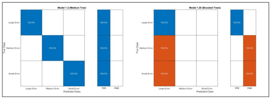
Figure 19.
Obtained confusion matrices for all sites based on the best and the worst classifier.
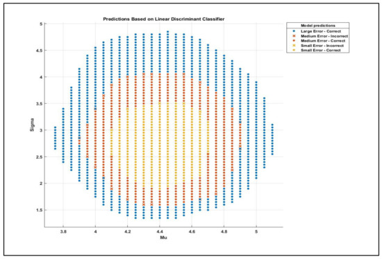
Figure 20.
Scatter plot shows that the uncorrected prediction occurs on the edge of two classes when the accuracy is high (90%).
A confusion matrix is a square matrix that is divided into n × n, where n is the number of classes. In this paper, low error, medium error, and large error were the three classes. Thus, the resulting confusion matrix was 3 × 3. However, it can be observed that the percentage of prediction for each class in this matrix is contained inside a square, where the reflection of this square on the x-axis represents how this classifier classifies this class, while the reflection on the y-axis represents the true classification. The diagonal line of each matrix represents the accurate predictions, and the out-of-diagonal squares are the incorrect predictions. Regardless, some other classifier algorithms showed a good performance, where the accuracy was close to 100%. Interestingly, it was observed that for the classifiers with 90% accuracy, the misclassified points were those which were located at the boundary (edge) between two classes, as represented in Figure 20. Surprisingly, another observation that is in dire need to be mentioned is that in ML classification, the data sample for each class affects the accuracy. For instance, if a certain class contains merely one row of data (one case), while the other classes have a relatively higher sample of data, the prediction of this class will not be detected easily or maybe at all. For example, there is the best selection of µ and σ that achieves the best fit for each site. Hence, when a new class was created and named “Best”, this class was not predicted since it contained merely one case, while the other classes contained around 500 cases or more.
Figure 20 shows that there is a certain range of µ and σ that commences and achieves a small error between the estimated and observed data. Once the values of µ and σ exceed this range, another region representing a medium error will be entered. Finally, when the range of µ and σ exceeds the range of medium error, the last region will be entered, which represents a large error.
The overall number of inserted data refers to the number of observations that were inserted to be trained and tested, or in other words, the same as the sample size. However, the previous table can be summarized by two main figures, as represented in Figure 21 and Figure 22. Based on Table 9, the performance of 24 classifier algorithms was evaluated. Hence, from the accuracy and training time points of view, it was deduced that the medium tree classifier showed the most accurate and swiftest results for all sites, with an accuracy percentage of 100% and with minimal training time compared with the other classifier algorithms. It can predict the error level based on the given values of µ and σ. Therefore, the medium tree classifier is a second-to-none trustworthy classifier since it can effectively predict the error. On the other hand, the ensemble-boosted trees classifier shows poor and awful performance in predicting the error level based on the values of µ and σ of each site. Figure 19 shows the confusion matrices based on these two classifier algorithms, where for all sites, the same matrices were obtained for these two classifiers. These classifier algorithms were trained and tested automatically by the classification learner application in MATLAB software, and the prediction process was carried out by exporting the trained model into a workspace.
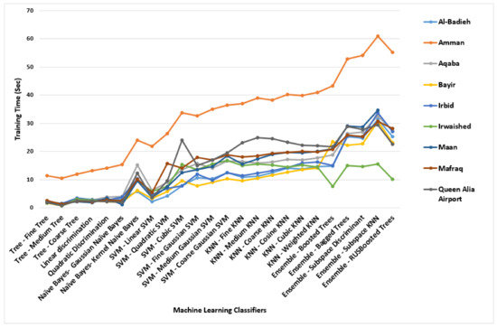
Figure 21.
Comparison between all 24 classifiers for all locations from the training time point of view.
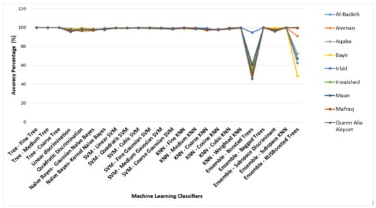
Figure 22.
Comparison between all 24 classifiers for all locations from an accuracy point of view.
Table 9.
The tested 24 classifiers for all candidate sites.
In the end, the usage of ML in this paper is justified since it was concluded based on Equations (11) and (12), which clarify how to calculate wind energy, that the energy calculation of wind depends on the turbine specifications, which are constant, in addition to the parameters of the proposed PDF. Hence, the precise selection of the parameter gives actual values for the wind energy regime and for the extractable energy from wind turbines. Otherwise, if the selection of the parameters is not accurate enough, all corresponding calculations cannot be trusted. Accordingly, the selection of these parameters is a critical phase and must be carried out wisely.
Hence, it was necessary to predict and double-check if the chosen parameters attained low error between the actual and the estimated wind speed values, and that was the role of the ML in this paper based on the most accurate classifier, which was the medium tree classifier.
4. Conclusions
This paper shed light on a PDF that is not regularly used in wind estimation, the normal PDF, which overwhelmed the most commonly used PDF in wind estimation, the Weibull PDF. The decision was made based on two performance indicators (RMSE and MAE). The goal of using these PDFs was to estimate the extractable energy from wind in nine sites in Jordan by the proper selection of the parameters of each PDF. The outcomes showed that Bayir is the richest wind source site. Finally, this paper used machine learning with 24 classifier algorithms for the purpose of predicting suitable parameters for each site based on previously trained data based on the k-fold cross-validation method. It was noticed that several classifier algorithms achieve an accuracy of 100%, which justifies the comparison between them based on the training time point of view. The medium tree classifier was the most accurate and swiftest classifier for all sites. On the contrary, the ensemble-boosted trees classifier was the worst one, with the lowest accuracy for the nine sites. Finally, it was observed that for the classifiers with accuracy in the range of 90%, the misclassified points were those which are located at the boundary (edge) between two classes.
Author Contributions
Methodology, H.H.D.; Formal analysis, H.H.D.; Investigation, A.A.-Q.; Writing—draft, H.H.D.; Writing—review & editing, A.A.-Q.; Supervision, A.A.-Q.; Project administration, A.A.-Q.; Funding acquisition, A.A.-Q. All authors have read and agreed to the published version of the manuscript.
Funding
This research received no external funding.
Institutional Review Board Statement
Not applicable.
Informed Consent Statement
Not applicable.
Data Availability Statement
Data available on request.
Acknowledgments
The authors would like to acknowledge Yarmouk University for their support in this research study.
Conflicts of Interest
The authors declare no conflict of interest.
References
- Al-Mhairat, B.; Al-Quraan, A. Assessment of Wind Energy Resources in Jordan Using Different Optimization Techniques. Processes 2022, 10, 105. [Google Scholar] [CrossRef]
- Al-Quraan, A.; Al-Qaisi, M. Modelling, Design and Control of a Standalone Hybrid PV-Wind Micro-Grid System. Energies 2021, 14, 4849. [Google Scholar] [CrossRef]
- Alrwashdeh, S.S. Energy sources assessment in Jordan. Results Eng. 2022, 13, 100329. [Google Scholar] [CrossRef]
- Stephan, A.; Stephan, L. Achieving net zero life cycle primary energy and greenhouse gas emissions apartment buildings in a Mediterranean climate. Applied Energy 2020, 280, 115932. [Google Scholar] [CrossRef]
- Thormark, C. A low energy building in a life cycle—Its embodied energy, energy need for operation and recycling potential. Build. Environ. 2002, 37, 429–435. [Google Scholar] [CrossRef]
- Arvesen, A.; Hertwich, E.G. More caution is needed when using life cycle assessment to determine energy return on investment (EROI). Energy Policy 2015, 76, 1–6. [Google Scholar] [CrossRef]
- Sahu, O. Sustainable and clean treatment of industrial wastewater with microbial fuel cell. Results Eng. 2019, 4, 100053. [Google Scholar] [CrossRef]
- Bull, S.R. Renewable energy today and tomorrow. Proc. IEEE 2001, 89, 1216–1226. [Google Scholar] [CrossRef]
- Neupane, D.; Kafle, S.; Karki, K.R.; Kim, D.H.; Pradhan, P. Solar and wind energy potential assessment at provincial level in Nepal: Geospatial and economic analysis. Renew. Energy 2022, 181, 278–291. [Google Scholar] [CrossRef]
- Emblemsvåg, J. Wind energy is not sustainable when balanced by fossil energy. Appl. Energy 2022, 305, 117748. [Google Scholar] [CrossRef]
- Wind Energy Project Analysis Clean Energy Project Analysis: Retscreen ® Engineering & Cases Textbook. Available online: https://unfccc.int/resource/cd_roms/na1/mitigation/Module_5/Module_5_1/b_tools/RETScreen/Manuals/Wind.pdf (accessed on 11 January 2023).
- Imdadullah; Alamri, B.; Hossain, M.A.; Asghar, M.S.J. Electric Power Network Interconnection: A Review on Current Status, Future Prospects and Research Direction. Electronics 2021, 10, 2179. [Google Scholar] [CrossRef]
- Bitar, E.Y.; Rajagopal, R.; Khargonekar, P.P.; Poolla, K.; Varaiya, P. Bringing Wind Energy to Market. IEEE Trans. Power Syst. 2012, 27, 1225–1235. [Google Scholar] [CrossRef]
- Saidur, R.; Rahim, N.A.; Islam, M.R.; Solangi, K.H. Environmental impact of wind energy. Renew. Sustain. Energy Rev. 2011, 15, 2423–2430. [Google Scholar] [CrossRef]
- Billinton, R.; Gao, Y. Multistate Wind Energy Conversion System Models for Adequacy Assessment of Generating Systems Incorporating Wind Energy. IEEE Trans. Energy Convers. 2008, 23, 163–170. [Google Scholar] [CrossRef]
- Varun; Prakash, R.; Bhat, I.K. Energy, economics and environmental impacts of renewable energy systems. Renew. Sustain. Energy Rev. 2009, 13, 2716–2721. [Google Scholar] [CrossRef]
- Kikuchi, R. Adverse impacts of wind power generation on collision behaviour of birds and anti-predator behaviour of squirrels. J. Nat. Conserv. 2008, 16, 44–55. [Google Scholar] [CrossRef]
- Sadorsky, P. Wind energy for sustainable development: Driving factors and future outlook. J. Clean. Prod. 2021, 289, 125779. [Google Scholar] [CrossRef]
- Renewable Capacity Statistics 2019. Irena.org. 2019. Available online: https://www.irena.org/publications/2019/Mar/Renewable-Capacity-Statistics-2019 (accessed on 11 January 2023).
- Statistics Time Series. Available online: https://www.irena.org/Statistics/View-Data-by-Topic/Capacity-and-Generation/Statistics-Time-Series (accessed on 11 January 2023).
- Siddique, S.; Wazir, R. A review of the wind power developments in Pakistan. Renew. Sustain. Energy Rev. 2016, 57, 351–361. [Google Scholar] [CrossRef]
- Alrwashdeh, S.S. Map of Jordan governorates wind distribution and mean power density. Int. J. Eng. Technol. 2018, 7, 1495. [Google Scholar] [CrossRef]
- Alsaad, M.A. Wind energy potential in selected areas in Jordan. Energy Convers. Manag. 2013, 65, 704–708. [Google Scholar] [CrossRef]
- Dalabeeh, A.S.K. Techno-economic analysis of wind power generation for selected locations in Jordan. Renew. Energy 2017, 101, 1369–1378. [Google Scholar] [CrossRef]
- Al-omary, M.; Kaltschmitt, M.; Becker, C. Electricity system in Jordan: Status & prospects. Renew. Sustain. Energy Rev. 2018, 81, 2398–2409. [Google Scholar] [CrossRef]
- Ammari, H.D.; Al-Rwashdeh, S.S.; Al-Najideen, M.I. Evaluation of wind energy potential and electricity generation at five locations in Jordan. Sustain. Cities Soc. 2015, 15, 135–143. [Google Scholar] [CrossRef]
- Bataineh, K.M.; Dalalah, D. Assessment of wind energy potential for selected areas in Jordan. Renew. Energy 2013, 59, 75–81. [Google Scholar] [CrossRef]
- Feilat, E.A.; Azzam, S.; Al-Salaymeh, A. Impact of large PV and wind power plants on voltage and frequency stability of Jordan’s national grid. Sustain. Cities Soc. 2018, 36, 257–271. [Google Scholar] [CrossRef]
- National Electric Power Company (NEPCO), Annual Report; NEPCO: Amman, Jordan, 2021.
- Online Store and Quote Request—The Wind Power—Wind Energy Market Intelligence. Available online: https://www.thewindpower.net/store_en.php (accessed on 11 January 2023).
- Filom, S.; Radfar, S.; Panahi, R. A Comparative Study of Different Wind Speed Distribution Models for Accurate Evaluation of Onshore Wind Energy Potential: A Case Study on the Southern Coasts of Iran. Energy Fuel Technol. 2020. [Google Scholar] [CrossRef]
- Mazzeo, D.; Oliveti, G.; Labonia, E. Estimation of wind speed probability density function using a mixture of two truncated normal distributions. Renew. Energy 2018, 115, 1260–1280. [Google Scholar] [CrossRef]
- Li, M.; Li, X. MEP-type distribution function: A better alternative to Weibull function for wind speed distributions. Renew. Energy 2005, 30, 1221–1240. [Google Scholar] [CrossRef]
- Stathopoulos, T.; Alrawashdeh, H.; Al-Quraan, A.; Blocken, B.; Dilimulati, A.; Paraschivoiu, M.; Pilay, P. Urban wind energy: Some views on potential and challenges. J. Wind. Eng. Ind. Aerodyn. 2018, 179, 146–157. [Google Scholar] [CrossRef]
- Al-Masri, H.M.K.; Al-Quraan, A.; AbuElrub, A.; Ehsani, M. Optimal Coordination of Wind Power and Pumped Hydro Energy Storage. Energies 2019, 12, 4387. [Google Scholar] [CrossRef]
- Usta, I. An innovative estimation method regarding Weibull parameters for wind energy applications. Energy 2016, 106, 301–314. [Google Scholar] [CrossRef]
- Al-Quraan, A.; Al-Mahmodi, M.; Radaideh, A.; Al-Masri, H.M.K. Comparative study between measured and estimated wind energy yield. Turk. J. Electr. Eng. Comput. Sci. 2020, 28, 2926–2939. [Google Scholar] [CrossRef]
- Al-Quraan, A.; Stathopoulos, T.; Pillay, P. Comparison of wind tunnel and on site measurements for urban wind energy estimation of potential yield. J. Wind. Eng. Ind. Aerodyn. 2016, 158, 1–10. [Google Scholar] [CrossRef]
- Kevin, O.O.; Otumba, E.; David, A.A.; Matuya, J. Fitting Wind Speed to a Two Parameter Distribution Model Using Maximum Likelihood Estimation Method. Int. J. Stat. Distrib. Appl. 2020, 6, 57. [Google Scholar] [CrossRef]
- Blažević, R. Statistical Analysis and Assessment of Wind Energy Potential in Sarajevo, Bosnia and Herzegovina. Teh. Vjesn.-Tech. Gaz. 2020, 28, 71–83. [Google Scholar]
- Boro, D.; Thierry, K.; Kieno, F.P.; Bathiebo, J. Assessing the Best Fit Probability Distribution Model for Wind Speed Data for Different Sites of Burkina Faso. Curr. J. Appl. Sci. Technol. 2020, 39, 71–83. [Google Scholar] [CrossRef]
- Saeed, M.A.; Ahmed, Z.; Zhang, W. Optimal approach for wind resource assessment using Kolmogorov–Smirnov statistic: A case study for large-scale wind farm in Pakistan. Renew. Energy 2021, 168, 1229–1248. [Google Scholar] [CrossRef]
- Bidaoui, H.; Abbassi, I.E.; Bouardi, A.E.; Darcherif, A. Wind Speed Data Analysis Using Weibull and Rayleigh Distribution Functions, Case Study: Five Cities Northern Morocco. Procedia Manuf. 2019, 32, 786–793. [Google Scholar] [CrossRef]
- Abeysirigunawardena, D.S.; Gilleland, E.; Bronaugh, D.; Wong, P. Extreme wind regime responses to climate variability and change in the inner south coast of British Columbia, Canada. Atmosphere-Ocean 2009, 47, 41–62. [Google Scholar] [CrossRef]
- Baloch, Z.A.; Tan, Q.; Kamran, H.W.; Nawaz, M.A.; Albashar, G.; Hameed, J. A multi-perspective assessment approach of renewable energy production: Policy perspective analysis. Environ. Dev. Sustain. 2021, 24, 2164–2192. [Google Scholar] [CrossRef]
- Sumair, M.; Aized, T.; Gardezi, S.A.R.; Bhutta, M.M.A.; Rehman, S.M.S.; ur Rehman, S.U. Comparison of three probability distributions and techno-economic analysis of wind energy production along the coastal belt of Pakistan. Energy Explor. Exploit. 2020, 39, 2191–2213. [Google Scholar] [CrossRef]
- Hemalatha, S.; Selwyn, T.S. Computation of mechanical reliability for Sub- assemblies of 250 kW wind turbine through sensitivity analysis. Mater. Today Proc. 2021, 46, 3180–3186. [Google Scholar] [CrossRef]
- Trevisi, F.; McWilliam, M.; Gaunaa, M. Configuration optimization and global sensitivity analysis of Ground-Gen and Fly-Gen Airborne Wind Energy Systems. Renew. Energy 2021, 178, 385–402. [Google Scholar] [CrossRef]
- Gupta, A.; Mishra, P.; Pandey, C.; Singh, U.; Sahu, C.; Keshri, A. Descriptive Statistics and Normality Tests for Statistical Data. Ann. Card. Anaesth. 2019, 22, 67. [Google Scholar] [CrossRef]
- Viti, A.; Terzi, A.; Bertolaccini, L. A practical overview on probability distributions. J. Thorac. Dis. 2015, 7, E7–E10. [Google Scholar] [CrossRef]
- Serban, A.; Paraschiv, L.S.; Paraschiv, S. Assessment of wind energy potential based on Weibull and Rayleigh distribution models. Energy Rep. 2020, 6, 250–267. [Google Scholar] [CrossRef]
- Honrubia, A.; Vigueras, A.; Gomez, E.; Mejıas, M.; Lainez, I. Comparative analysis between lidar technologies and common wind speed meters. In Proceedings of the World Wind Energy Conference, Istanbul, Turkey, 27 June 2010. [Google Scholar]
- Manwell, J.F.; Mcgowan, J.G.; Rogers, A.L. Wind Energy Explained: Theory, Design and Application; John Wiley & Sons, Ltd.: Chichester, UK, 2011; Available online: https://www.wiley.com/en-us/Wind+Energy+Explained%3A+Theory%2C+Design+and+Application%2C+2nd+Edition-p-9780470015001 (accessed on 11 January 2023).
- An, Y.; Quan, Y.; Gu, M. Field Measurement of Wind Characteristics of Typhoon Muifa on the Shanghai World Financial Center. Int. J. Distrib. Sens. Netw. 2012, 8, 893739. [Google Scholar] [CrossRef]
- Bagiorgas, H.S.; Mihalakakou, G.; Rehman, S.; Al-Hadhrami, L.M. Wind power potential assessment for three buoys data collection stations in the Ionian Sea using Weibull distribution function. Int. J. Green Energy 2015, 13, 703–714. [Google Scholar] [CrossRef]
- GPS Coordinates of Jordan Latitude Longitude Elevation—CountryCoordinate.com. Available online: https://www.countrycoordinate.com/country-jordan/ (accessed on 11 January 2023).
- Çakmakçı, B.A.; Hüner, E. Evaluation of wind energy potential: A case study. Energy Sources Part A Recovery Util. Environ. Eff. 2020, 44, 834–852. [Google Scholar] [CrossRef]
- Masters, G.M. Renewable and Efficient Electric Power Systems; Wiley-Blackwell: Chichester, UK, 2013. [Google Scholar]
- Forbes, C.; Evans, M.G.A.; Hastings, N.A.; Peacock, B. Statistical Distributions; Wiley: Hoboken, NJ, USA, 2011. [Google Scholar]
- Weisstein, E.W. Normal Distribution. Available online: https://mathworld.wolfram.com/NormalDistribution.html (accessed on 11 January 2023).
- Milan, P.; Wächter, M.; Barth, S.; Peinke, J. Power curves for wind turbines. Wind. Power Gener. Wind. Turbine Des. 2010, 44, 595–612. [Google Scholar] [CrossRef]
- Al-Quraan, A.; Al-Mhairat, B. Intelligent Optimized Wind Turbine Cost Analysis for Different Wind Sites in Jordan. Sustainability 2022, 14, 3075. [Google Scholar] [CrossRef]
- Eminoglu, U.; Turksoy, O. Power curve modeling for wind turbine systems: A comparison study. Int. J. Ambient. Energy 2019, 42, 1912–1921. [Google Scholar] [CrossRef]
- Mölders, N.; Khordakova, D.; Dlugi, R.; Kramm, G. Sustainability of Wind Energy under Changing Wind Regimes—A Case Study. Atmos. Clim. Sci. 2016, 6, 158–173. [Google Scholar] [CrossRef]
- Mellit, A.; Kalogirou, S.A. Artificial intelligence techniques for photovoltaic applications: A review. Prog. Energy Combust. Sci. 2008, 34, 574–632. [Google Scholar] [CrossRef]
- Singh, S.; Patel, B.; Upadhyay, R.K.; Singh, N.K. Improvement of process performance of powder mixed electrical discharge machining by optimisation—A Review. Adv. Mater. Process. Technol. 2021, 8, 3074–3104. [Google Scholar] [CrossRef]
- Katoch, S.; Chauhan, S.S.; Kumar, V. A review on genetic algorithm: Past, present, and future. Tools Appl. 2021, 80, 8091–8126. [Google Scholar] [CrossRef]
- Liu, Y.; Passino, K.M. Biomimicry of Social Foraging Bacteria for Distributed Optimization: Models, Principles, and Emergent Behaviors. J. Optim. Theory Appl. 2002, 115, 603–628. [Google Scholar] [CrossRef]
- Li, Z.; Wang, Z. Bacterial Foraging Algorithm With Potential Field Guidance Mechanism. Research Square 2021. [Google Scholar] [CrossRef]
- Odziemczyk, W. Application of simulated annealing algorithm for 3D coordinate transformation problem solution. Open Geosci. 2020, 12, 491–502. [Google Scholar] [CrossRef]
- Venkateswaran, C.; Ramachandran, M.; Ramu, K.; Prasanth, V.; Mathivanan, G. Application of Simulated Annealing in Various Field. Mater. Its Charact. 2022, 1, 100299. [Google Scholar] [CrossRef]
- Mewada, K.M.; Sinhal, A.; Verma, B. Adaptive neuro-fuzzy inference system (ANFIS) based software evaluation. Int. J. Comput. Sci. Issues (IJCSI) 2013, 10, 244. [Google Scholar]
- Onu, C.E.; Nweke, C.N.; Nwabanne, J.T. Modeling of thermo-chemical pretreatment of yam peel substrate for biogas energy production: RSM, ANN, and ANFIS comparative approach. Appl. Surf. Sci. Adv. 2022, 11, 100299. [Google Scholar] [CrossRef]
- Zeinalnezhad, M.; Chofreh, A.G.; Goni, F.A.; Klemeš, J.J. Air pollution prediction using semi-experimental regression model and Adaptive Neuro-Fuzzy Inference System. J. Clean. Prod. 2020, 261, 121218. [Google Scholar] [CrossRef]
- Hodson, T.O. Root mean square error (RMSE) or mean absolute error (MAE): When to use them or not. Geosci. Model Dev. 2022, 15, 5481–5487. [Google Scholar] [CrossRef]
- Tamilarasi, P.; Rani, R. Diagnosis of Crime Rate against Women using k-fold Cross Validation through Machine Learning. In Proceedings of the 2020 Fourth International Conference on Computing Methodologies and Communication (ICCMC), Erode, India, 11–13 March 2020. [Google Scholar] [CrossRef]
- Rodriguez, J.D.; Perez, A.; Lozano, J.A. Sensitivity Analysis of k-Fold Cross Validation in Prediction Error Estimation. IEEE Trans. Pattern Anal. Mach. Intell. 2010, 32, 569–575. [Google Scholar] [CrossRef]
- Breck, E.; Polyzotis, N.; Roy, S.; Whang, S.; Zinkevich, M. Data Validation for Machine Learning. In Proceedings of the 2nd SysML Conference, Palo Alto, CA, USA, 31 March–2 April 2019. [Google Scholar]


Disclaimer/Publisher’s Note: The statements, opinions and data contained in all publications are solely those of the individual author(s) and contributor(s) and not of MDPI and/or the editor(s). MDPI and/or the editor(s) disclaim responsibility for any injury to people or property resulting from any ideas, methods, instructions or products referred to in the content. |
© 2023 by the authors. Licensee MDPI, Basel, Switzerland. This article is an open access article distributed under the terms and conditions of the Creative Commons Attribution (CC BY) license (https://creativecommons.org/licenses/by/4.0/).