Abstract
Based on the Spatial Durbin Model (SDM), this study evaluates the spatial spillover effect of PM2.5 concentration in Beijing–Tianjin–Hebei (BTH) and its surrounding areas from 2000 to 2016, analyzes its main influencing factors and verifies the Environmental Kuznets Curve (EKC). In addition, Social Network Analysis (SNA) is used to measure the regional air pollution transmission network. The results are as follows: (1) A significant inverted U-shaped EKC with spatial spillover effect between the sampled 48 cities was verified. (2) Industrial structure had both local and spillover effects on air pollution with a U-shaped curve; technological progress exerted a negative spillover effect on air pollution, while traffic evidenced positive local and spillover effects; meteorological conditions showed different impacts on air pollution. (3) Heze, Tianjin, Xingtai, Shijiazhuang and Liaocheng are the top five cities in the centrality of the air pollution correlation network, indicating air pollution in these cities have significant impacts on other cities within the network; while Sanmenxia, Weihai, Yuncheng, Langfang and Zhumadian are the bottom five cities, which indicates that the air pollution of these cities has the least correlation with other cities. The policy suggestions for 48 cities involve: building up a regional joint prevention and control mechanism, enhancing the supervision of cities located in the centrality of the air pollution correlation network, accelerating high-tech and service-oriented industrialization, encouraging technological innovation in energy conservation and environmental protection and implementing vehicle regulation.
1. Introduction
The environmental consequences of four decades of urbanization and economic development have become a major concern in China [1]. Air pollution, represented by haze pollution, is one of the most noticeable environmental problems, leading to policy challenges for the Chinese government [2,3,4]. According to current literature, air pollution is recognized as a regional environmental problem, contributed to by pollutants, typically represented by PM2.5 [5,6]. In addition, considering that air pollution also has a negative impact on people’s health [7,8,9], the United Nations proposed 17 Sustainable Development Goals (SDGs) in 2015 to effectively address the three dimensions of social, economic and environmental issues. Goal 13, taking urgent action to address climate change and its impacts, focuses on the impact of climate change on economic development, natural resources and poverty alleviation. How to deal with climate change has become a thorny issue for achieving sustainable development.
The Beijing–Tianjin–Hebei (BTH) region and its surrounding areas is one of the most polluted areas in China, with the highest annual average concentration of PM2.5 (43 µg/m3) among all key regions of China in 2021. A substantial gap still remains between the current annual average concentration in this region and the national standard for PM2.5 (35 µg/m3) [10]. In 2010, the General Office of the State Council (GOSC) proposed a joint strategy of air pollution prevention and control for the first time. The BTH region was clarified as a key region. It is vital to explore the relationship between economy and air pollution in this region. In 2013, the GOSC issued The Five-Year Action Plan for Air Pollution and Control (The Ten Articles), defining the BTH region and its surrounding areas. In 2017, the BTH region and its surrounding areas, consisting of two municipalities directly under the Central Government and 26 cities, were identified as air pollution transmission channels by the Ministry of Ecology and Environment (MEE), for more efficient air pollution control. In 2018, the State Council issued the Three-Year Action Plan for Winning the Blue Sky Defense Battle (Three-Year Action Plan) in June, taking the BTH region and its surrounding areas as a key region, which thus, enhanced air pollution prevention and control in the 2 + 26 cities (known as the 2 + 26 policy); in July, it further established an integrated leading group on air quality control for the BTH region and its surrounding areas, entitled the Air Pollution Prevention and Control Steering Group of the BTH Region and Surrounding Areas.
Strict emission reduction policies have been introduced in the BTH region and its surrounding areas, especially in the 2 + 26 cities, which indeed improves the air quality in this area. In 2021, the number of heavily polluted days in cities decreased by 51% compared with 2015, and PM2.5 decreased by 18.9% compared with 2020 [11]. Among these policies, strengthened supervision of air pollution was one of the most typical policies. It has targeted “small, scattered, unregulated and high-pollution” enterprises since April 2017. These enterprises are characterized as small scale, poor technology, scattered distribution, high pollution and low efficiency and occupying a certain market space due to low cost [12]. In 2017, 62,000 “small, scattered, unregulated and high-pollution” enterprises, 36,000 gas-related environmental problems, and 20,000 key environmental problems were supervised [13]. Among all supervised enterprises, 73.5% of them had been banned, 23.5% had been upgraded, and 1.2% had moved to industrial zones [14]. Enhanced supervision led to the relief of air pollution, but also to the shutdown of enterprises on a large scale. Economic losses might happen due to the production stoppage of these enterprises in the short term [10]. Did it mean that air quality improvement in this region came at the cost of the economy? To discuss the relationship between economic development and air pollution, the Environmental Kuznets Curve (EKC) hypothesis was worth verifying in this region to provide better suggestions for current and future policies.
The research on EKC started with Grossman and Krueger (1991) [15], in a study on the environmental impact of the North American Free Trade Agreement (NAFTA). They put forward the EKC hypothesis, adapted from the original Kuznets Curve [16], which described an inverted U-shaped relationship between income and inequality. The EKC hypothesis reflects the relationship between economic development and environmental degradation, with the inverted U-shape positing that environmental degradation first increases as a nation’s income grows and then reaches a turning point, after which, the environment begins to improve [17]. Extensive research has been carried out for the verification of the EKC hypothesis [18]. The inverted U-shape relationship between economic growth and air pollution has been verified in many regions [19,20,21]. Chen and Taylor (2020) confirmed the EKC hypothesis regarding chromium emissions and economic indicators in Singapore [22]. According to Dong et al. (2018), in 1970–2016, 13 of the 14 Asia Pacific countries showed inverted U-shaped relationships between per capita emissions of carbon dioxide (CO2) and per capita GDP [23].
Existing literature has verified the relationship between economic development and air pollution at a national [24,25], provincial or state level [26,27], and municipal level [28,29]. Adopting provincial data in China from 1990 to 2012, Wang et al. (2016) found evidence of an inverted U-shaped relationship between economic growth and sulfur dioxide (SO2) emissions, but not of the EKC hypothesis between urbanization and SO2 emissions [30]. Zhou et al. (2019) explored the impact of urbanization on CO2 emissions in 16 cities of the Yangtze River Delta (YRD), and proved an EKC association [31]. Wang and Liu (2017) confirmed the EKC hypothesis in China with an inverted U-shaped curve of per capita GDP and estimated city-level CO2 emissions [32].
Intuitively, the EKC hypothesis of an inverted U-shaped pattern to pollution makes sense, in that citizens focus on immediate subsistence needs when they are poor but shift to life quality issues, e.g., environmental improvement, as they become wealthier. Testing for the existence of EKC, however, reveals how complex the correlation really is. For one thing, the EKC hypothesis may be invalid in some regions [33,34]. Panel data from 22 Latin American and Caribbean countries for the period 1990–2011 showed no EKC relationship between income and energy consumption [35]. Moreover, empirical examination confirmed more EKC forms, i.e., a U-shape [36,37], N-shape [38,39,40], inverted N-shape [41,42], etc. Özokcu and Özdemir (2017) demonstrated both N-shaped and inverted N-shaped curves for income and CO2 emissions in 26 OECD countries and 52 emerging countries [43].
The existing literature adopted the panel data model for the validation of the EKC hypothesis, regarding samples as independent individuals without interaction. However, haze pollution has a characteristic of short-term cross-boundary transmission, indicating an interactional relationship between regions [44]. Traditional EKC studies failed to capture the spillover effect of air pollution, especially for research at the provincial and city level. Some scholars began to incorporate the spatial effect into EKC research [45,46,47]. Ding et al. (2019) compared nonspatial and spatial EKC models in 13 cities of the BTH region from 1998 to 2016, and concluded that the EKC turning points come later under spatial EKC [48]. Balado-Naves et al. (2018) constructed both standard and spatial EKC models for income and CO2 emissions in seven different sets of countries, with a database of 173 countries for 1990–2014 [49]. Their results supported direct EKC in all regions, and indirect EKC for the world, Europe and Asia. With multiple semiparametric spatial autoregressive models, Xie et al. (2019) confirmed the strong positive spatial spillover of PM2.5 concentration, and an inverted U-shaped EKC for economic growth and PM2.5 contamination of 249 Chinese cities in 2015 [50].
Based on the existence of a spatial spillover effect in previous studies, this research tried to test the EKC hypothesis from a spatial perspective. The Spatial Durbin Model (SDM) is widely used to evaluate the spatial effect [51,52,53]. The influence of urbanization within and across cities on PM2.5 concentration was proven by Du et al. (2019), adopting SDM with regional data in the BTH region over the period 2000–2015 [54]. Zhu et al. (2017) found a positive impact of foreign direct investment (FDI) on SO2 emissions with SDM in the BTH region from 2000 to 2013 [55]. Du et al. (2018) used SDM and other spatial regression models to examine the direct and spillover effects of urbanization on PM2.5 concentration in three urban agglomerations, including the BTH region, the Yangtze River Delta (YRD) and the Pearl River Delta (PRD) [56]. SDM measured intraregional spillover by introducing spatial lags of both independent and dependent variables, which is suitable for evaluating the spillover effect of economic development and air pollution in this research [57,58].
Based on existing studies, this paper tries to explore the following the problems: the existence of the EKC hypothesis in the BTH region, the impact of different indicators on air pollution such as industry, technology, meteorological factors, etc., and the correlation network of 48 cities in the BTH region. The contributions of this study are as follows. First, based on testifying the EKC hypothesis, this paper further discusses the local and spillover effect of the relationship between economic development and air pollution and the necessity of coordinated air pollution prevention and control. Secondly, diverse influencing factors were considered as control variables in this research, such as industrial structure, technological innovation, traffic and meteorological conditions. Thirdly, the characteristics of the air pollution correlation network were also evaluated by using Social Network Analysis (SNA) model, as to put forward corresponding policy suggestions.
2. Methodology
2.1. Research Area
The BTH region and its surrounding areas is in the northeast of China, with longitude and latitude between 110°40′ E~123°30′ E and 31°20′ N~42°40′ N. It includes 2 municipalities directly under the central government and 4 provinces: Beijing, Tianjin, Hebei, Henan, Shandong and Shanxi. Based on the data availability, 48 cities were selected as samples (see in Figure 1). The population of 48 cities increased from 262.36 million in 2000 to 299.83 million in 2016, with a growth rate of 14.28%. The per capita GDP of the sampled region enhanced from 4.15 billion yuan in 2000 to 27.22 billion yuan in 2016, realizing rapid economic growth. The average PM2.5 concentration in BTH region was 71 μg/m3 in 2016, representing a 33.0% decline compared to 2013. Air quality in the BTH region has experienced continuous improvement from its status as high pollution.
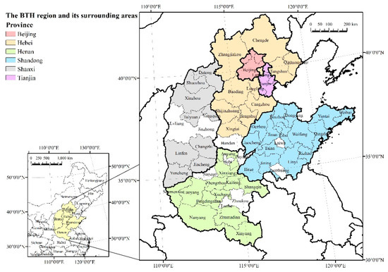
Figure 1.
Spatial layout of selected samples in the BTH region and its surrounding areas.
2.2. Moran’s I Index
It is necessary to examine the spillover effect of key indicators in the sampled region to confirm the chosen spatial methods. Moran’s I index has extensive application in spatial econometrics to calculate the spatial dependence [59,60]. Global Moran’s I index was used to measure the spatial autocorrelation of the economy and air pollution. The equation is as follows:
where n denotes the numbers of cities; wij is the element at row i and column j of the spatial weight matrix; xi and xj are the PM2.5 concentration or per capita GDP of city i and j, which indicate air pollution and economic development, respectively; represents average PM2.5 concentration or GDP of all cities; and S2 is the variance of PM2.5 concentration or per capita GDP of all cities. Moran’s I index values range from −1 to 1, where I > 0 indicates a positive autocorrelation of PM2.5 concentration or per capita GDP among cities, and I < 0 means a negative autocorrelation. No autocorrelations exist when I = 0.
2.3. Spatial Econometrics Model
2.3.1. Traditional Panel EKC
Most scholars adopted traditional panel data model to verify the EKC hypothesis proposed by Grossman and Krueger (1991), in which quadratic functions were mostly used to test the EKC hypothesis. Quadratic functions had a general form as follows:
where POLLUit and PCGit stand for air pollution and economic development, respectively; X denotes control variables; α0 is a constant term; α1 and α2 are parameters of explanatory variables; β is the parameter of control variables; ηi and δt denote the individual and time fixed effect respectively; εit is error term. When α2 = 0, α1 ≠ 0, POLLUit and PCGit show linear relationships; when α1 > 0, α2 < 0, POLLUit and PCGit present inverted U-shaped quadratic relationships; when α1 < 0, α2 > 0, Pit and Git demonstrate quadratic relationships with a U-shaped curve; when α1 = α2 = 0, no relationship exists between POLLUit and PCGit, which means no impact of economic development on air pollution. Variables in Equation (2) are all logarithmic.
lnPOLLUit = α0 + α1lnPCGit + α2(lnPCGit)2 + βlnX + ηi + δt + εit
2.3.2. Improved EKC Model with Spatial Effect
The diffusion and spillover of air pollution explained the necessity of incorporating spatial spillover into traditional panel EKC model. SDM was introduced in this research to construct the improved spatial EKC model. The general form of SDM is as follows:
where y and X denote dependent variables and independent variables, respectively; W is the matrix of spatial weight to represent the spatial correlation between cities; Wy and WX are the spatial lag of dependent variables and independent variables, respectively; α is the constant term; ln denotes identity matrix of order n; ρ, β, θ are parameters of variables; ε is the error term. Based on existing literature, binary adjacent matrix was adopted as spatial weight matrix [61]:
y = αln + ρWy + βX + WXθ
Referring to related research and data availability, industrial structure, technological progress, traffic, and meteorological factors (wind, rain, temperature and humidity) were taken as control variables in the model. Based on Equation (2) and Equation (3), the improved spatial EKC model is expected to be as follows:
where ISit, TPit and TRit indicate industrial structure, technological progress and traffic, respectively; MWit, RAit, TEMit and HUMit stand for wind, rain, temperature and humidity, respectively; α is a constant term.
SDM must satisfy the assumption of θ ≠ 0 and θ + βρ ≠ 0, otherwise it will be reduced to a spatial autoregressive model (SAR) and spatial error model (SEM) if either assumption is not satisfied.
(i) θ = 0: SDM is simplified into SAR as
y = ρWy + αιn + Xβ + WXθ + ε
(ii) θ + βρ = 0: SDM is simplified into a SEM as
y = Xβ + ε, ε = ρWε + u
(iii) θ = 0 and θ + βρ = 0: SDM is simplified to a nonspatial panel model, as in Equation (2).
Thus, several tests were needed to verify the applicability of spatial SDM, including LM test, Hausman test, Wald test and the LR test [62].
Maximum likelihood estimation (MLE), instead of ordinary least squares (OLS), was adopted in spatial econometric model due to the endogeneity of spatial-lagged dependent variables [63,64]. The existence of a spatial effect leads to bias of marginal effect if only focusing on coefficients of independent variables. To avoid biased conclusions, the spatial spillover effect is divided into the direct effect and indirect effect by partial derivative. The SDM was rewritten into the following:
Yit = (I − ρW)−1(Xitβ + WXitθ + ηi + δt + εit)
The partial derivative matrix of yi on Xi (i = 1, 2, …,n) is as follows:
where xik (k = 1,2,…, m) indicates independent variables in Equation (5); wij is the element at row i and column j of W; the diagonal elements of matrix A represents the impact of independent variables of city i on the dependent variable of city i, which is a direct effect; the off-diagonal elements of matrix A are the impact of independent variables of city j on the dependent variable of city i, which is an indirect effect; the sum of the direct effect and the indirect effect is the total effect.
2.4. Social Network Analysis
Social Network Analysis (SNA) is widely adopted in research related to relationship between different units, which could measure the correlation of a certain network or identify the characteristics of a certain unit within the network [65,66]. This paper applied SNA to evaluate the correlations of PM2.5 between the sampled 48 cities within the H region and its surrounding areas. The Gravity Model is introduced into SNA model for describing the variation of PM2.5’s social network in that it can include economy, society and geography elements comprehensively.
where, is the gravity of city i to city j in PM2.5 emission, stands for the contribution in PM2.5 emission of region i to region j, and denote the PM2.5 in region i and region j, respectively, representing air pollution. and are the annual GDP in region i and region j, respectively, both indicating economic development. and denote the permanent resident population in region i and region j, respectively, which shows the indicator of population. is the spatial distance between city i and city j, calculated by spherical distance between cities.
The indicators to measure relevance and robustness of network include: network density (Dn), network reachability (C) and graph efficiency (GE). Centrality analysis is used to explore the position and role of cities in the BTH region and its surrounding areas, including degree centrality (Cd), closeness centrality (Cc) and betweenness centrality (Cb).
where L denotes the sum of actual correlations in the network, N is the number of cities in the network, V represents actual number of unreachable pairs in the network, M defines the number of symmetrically reachable points in the network, max(M) is the maximum number of symmetrically reachable points in the network, n stands for the number of cities directly correlated with the certain city, bjk(i) stands for the ability of city i to control correlation between city j and k, and dij is the distance between city i and j.
2.5. Variables and Data
The definition of each variable is shown in Table 1. In this research, POLLU stands for air pollution, which is expressed by the annual PM2.5 concentration. PCG refers to economic development, indicating real per capita GDP. IS means industrial structure, which is indicated by the proportion of second industry. TP is technological progress, which is measured by annual total patent grants. TR means traffic, which is expressed by highway passenger quantity. Meteorological condition has four indicators: wind (MW), rain (RA), temperature (TEM) and humidity (HUM), which are indicated by annual maximum instantaneous wind speed, annual total rainy days, annual average temperature and annual average relevant humidity, respectively. Municipal level data in the sampled 48 cities of the BTH region and its surrounding areas from 2000 to 2016 were adopted and processed. Real per capita GDP was calculated by nominal GDP and its index with a base year of 2000.

Table 1.
Data sources and definition of variables and descriptive statistics.
The original data sources are as follows: PM2.5 concentration is from satellite data released by the Socioeconomic Data and Applications Center at Columbia University; nominal GDP, nominal GDP index, population at the end of the year, proportion of second industry, and annual highway passenger quantity are from Chinese Urban Statistical Yearbook (2001–2017) and local statistical yearbooks; annual total patent grant is from Chinese Research Data Services Platform (CNRDS); annual maximum instantaneous wind speed, annual total rainy days, annual average temperature and annual average relevant humidity are from China Meteorological Science Data Center. The data volume differs significantly according to the descriptive statistics of variables (see Table 1), which proves the necessity of a logarithm. All data were not missing and balanced.
3. Results
3.1. Result of Non-Spatial EKC
To ensure the validity of estimation, several unit root tests were adopted in this research to examine the stationarity of panel data. Table 2 shows the result of unit root tests, in which all test values were significant and evidenced stationary.
Table 2.
Results of unit root tests.
The results of nonspatial panel data are in Table 3. The EKC hypothesis existed when excluding spatial factors in the sampled cities of the BTH region and its surrounding areas, with an inverted-U shaped relationship between economic development and air pollution. The relationship between industrial structure and air pollution showed a U-shaped curve. Traffic, temperature and humidity had significantly positive impact on PM2.5 concentration within the region at the 1% significance level. The variables of technological progress, wind speed and rain did not pass the significance test in this non-spatial model.
Table 3.
Results of nonspatial panel model.
3.2. Spatial Autocorrelation
Global Moran’s I of PM2.5 concentration and per capita GDP (base year = 2000) were calculated, as shown in Table 4. Moran’s I indices all exceeded 0 and passed the test of significance under 0–1 spatial weight matrix. The significance of the positive spatial autocorrelation supported the spatial aggregation effect of the economy and air pollution in the sampled 48 cities, which further documented the necessity of spatial econometrics models. It was revealed that the spatial aggregation of air pollution was strengthened during 2000–2016. Moran’s I of POLLU in the BTH region and its surrounding areas fluctuated upward during 2000–2016, which was 0.604 in 2006, and 0.706 in 2016. Interannual changes of the Moran’s I of PCG was illustrated according to Table 3. It increased in the first 3 years, but decreased sharply from 2002 to 2005. It then showed a rising trend until reaching its peak (0.264) in 2010. The Moran’s I of per capita GDP was 0.257 in 2016, which slightly declined compared to that in 2000 (0.263). Significant spatial aggregation of PM2.5 concentration revealed the necessity of further consideration of spatial effects [67].
Table 4.
Results of global Moran’s I in the sampled 48 cities.
3.3. Results of SDM
3.3.1. Tests for SDM
Spatial diagnosis was tested for the validation of SDM. The calculated Moran’s I passed the significance test at 1%, which demonstrated the spatial effect of the constructed model and rejected the feasibility of simply constructing a nonspatial model. Statistics of LM test, including LM lag, LM error, robust LM lag, and robust LM error, were significant at the 1% level. Therefore, SAR and SEM were both applicable. SDM, thus, can be further considered in the following steps. The selected samples were not random, but based on government policy, being concentrated in the BTH region and its surrounding areas, so the conclusions would be difficult to verify in other regions. Thus, SDM with fixed effects was applicable in this research. The Wald and LR tests were used to guarantee non-degeneration of SDM into SAR or SEM (see Table 5). All Wald and LR tests were passed with a significance level of 1%, indicating the rationality of SDM in this research. Another LR test was employed to determine whether to consider individual fixed effects, time fixed effects, or both. Time fixed effects and individual fixed effects both passed the LR test at a 1% significance level. Therefore, both individual and time fixed effects should be taken into consideration. MLE should be used for regression, after eliminating individual effects through statistical transformation.
Table 5.
LM, Wald, and LR tests.
3.3.2. Results of Regression
Table 6 demonstrates the results of SDM under three spatial weight matrices. ρ remained significant at the 1% level, indicating a significant spatial spillover effect within the 48 cities. lnPCG and (lnPCG)2 showed no significant correlation with lnPOLLU, meaning that the EKC hypothesis failed in the region under this spatial weight matrix. However, the coefficients showed an inverted U-shaped relationship between economic development and air pollution [68]. The spatial lagged terms of lnPCG and (lnPCG)2 both passed significance tests, indicating an inverted U-shaped relationship between economic development of neighboring cities and local air pollution, which illustrated the spatial spillover effect of the EKC hypothesis. That is, the air quality of a certain city in the sampled cities of the BTH region and its surrounding areas was influenced by local economic development, as well as the economy of neighboring cities.
Table 6.
Regression results of SDM.
lnIS and (lnIS)2 passed the significance tests at the 1% and 5% significance level, respectively, while the spatial lagged term of them both passed the significance tests with 10% significance, which demonstrated a U-shaped curve with a spatial spillover effect between industrial structure and air pollution. Although lnTP failed the significance test, its spatial lagged term revealed negative impact at the 1% significance level, illustrating significant spatial spillover effect of technology progress. lnMW and lnRA demonstrated negative impact on air pollution at the 1% and 5% significance level, respectively; their spatial lagged term showed negative coefficient but failed the significance test. lnTR, and lnTEM all failed significance tests, which meant these variables have no significant local and spatial relationship with air pollution. lnHUM showed significant spillover effect at the 1% level, but non-significant local effect according to the estimation. Aiming at unbiased estimation, the results of effect decomposition are given in Table 7.
Table 7.
Results on direct, indirect, and total effects.
lnPCG and (lnPCG)2 had a direct effect on lnPOLLU at the 5% significance level, indicating an inverted U-shaped relationship between local economic development and local air pollution within the 48 cities in the BTH region and its surrounding areas. lnPCG and (lnPCG)2 both showed indirect effect on lnPOLLU at the 1% significance level, which illustrated an inverted U-shaped curve between economic development in neighboring cities and air pollution in local cities within the sampled region. As for the total effect, lnPCG and (lnPCG)2 also passed the significance tests at the 1% level, which demonstrated an inverted U-shaped relationship between economic development and air pollution from the regional perspective. lnIS and (lnIS)2 passed the significance tests at the 1% significance level with direct and indirect effect, showing a U-shaped curve between secondary industry in local and neighboring cities, and local air pollution. From regional perspective, lnIS and (lnIS)2 also demonstrated significant total effect on lnPOLLU at the 1% level, with U-shaped relationship. Although lnTP did not passed the significance test with direct effect, the negative coefficient indicated the existence of negative correlation between technological progress and air pollution in local cities. lnTP had negative indirect effect on lnPOLLU at the 1% significance level, illustrating the spillover effect of technological progress within the 48 cities. The total effect of lnTP was also negatively significant at the 5% significance level, which meant a negative impact of overall technological progress on PM2.5 concentration, that is, the development of technology in the sampled region would improve air pollution. lnTR demonstrated positive significance with direct effect and indirect effect at the 5% level, which indicated the local and spillover effect of traffic on air pollution in the 48 cities. lnTR showed positive total effect (5% significance level) within the sampled region, that is to say, traffic is harmful to the air pollution of the region on the whole.
The variables of meteorological conditions showed different estimated results [69]. lnMW showed a negative impact on local air pollution at the 5% significance level, which illustrated that strong wind alleviated air pollution in local cities. The indirect effect and total effect of lnMW did not pass the significance tests. lnRA had a negative correlation with lnPOLLU at 10% significance level, but showed no significant indirect effect and total effect on lnPOLLU. lnTEM had no significant direct effect on lnPOLLU, indicating the temperature did not have impact on local PM2.5 concentration from year scale. A positive spillover effect was evidenced at the 1% significance level, which indicated the rise of temperature in neighboring cities leaded to the increase of PM2.5 concentration in the local. Total effect showed positive correlation between the regional temperature and air pollution at the 1% significance level, indicating the higher the annual average temperature in the region, the more serious air pollution in the region, mainly due to the spillover effect of air pollution [70]. The rise of temperature in neighboring cities was conducive to air diffusion, which led to the spillover of air pollution from neighboring cities to the local. Although literature explained that high temperature weather makes air pollution less possible, once there is serious air pollution in some parts of the region, high temperature would more easily result in air pollution diffusion as air convection increased, instead of local settlement, which can spread the pollution in some cities into the whole region. lnHUM had positive direct effect at the 5% significance level, which indicated humidity in local cities would promote local air pollution. The indirect effect passed the significance test at the 1% level, demonstrating a strong spillover effect from neighboring cities to local cities in the region. The total effect also evidenced positive correlation between humidity and air pollution.
3.3.3. Effect Decomposition
The SDM results confirmed the EKC hypothesis in the sampled 48 cities of the BTH region and its surrounding areas from a spatial perspective, as the relationship between regional economic development and air pollution presented an inverted U-shaped curve. With the development of economy in local and neighboring cities, the PM2.5 concentration in the local within sampled regions went through two stages: rising to the inflexion point and then falling naturally. That is, an inverse relationship exists between economic development and air pollution during industrialization and urbanization. Coordination of regional economic development and air pollution occurs when the economy has developed to a higher level. The development of secondary industry in the local and neighboring cities will firstly relieve local air pollution, then lead to aggravation when it comes to the turning point, which presents a U-shaped curve. Technological progress is beneficial for air pollution improvement, while traffic has the opposite effect. The impact of meteorological conditions is mostly limited to local cities, such as wind, humidity and precipitation; meteorological variables with significant spillover effects include temperature and humidity.
Local economic development, industrial structure and traffic all have impacts on local air pollution [71]. It is reasonable for the government to put severe restrictions in place to encourage air pollution reduction, especially when air pollution is on the rise. The government must bring air pollution under control to minimize the damage to public health and to ecosystems. Besides, the spillover effects of economic development, industrial structure, technological progress and traffic in the BTH region and its surrounding areas should not be ignored. Strict environmental regulations in a single city cannot ensure complete improvement within the whole region due to the spillover effect. Regional joint prevention and control is a feasible solution in the BTH region and its surrounding areas, which involves adopting unified management of regional air pollution control [72]. Rather than dividing the scope of pollution control by administrative divisions, such a policy puts the emphasis on the integral development of the region. The MEE has implemented strict supervision of air pollution prevention and control in the “2 + 26” cities since 2017, with measures of shutdowns, upgrading, integration and relocation. From the perspective of heavy polluting industries, these measures would inevitably impact the GDP of related industries, especially the shutdowns of enterprises. However, according to existing literature, such supervision has no significant effect on local economic development. Besides, it is in line with the development progress of EKC in the long run. The supervision of “small, scattered, unregulated and high-pollution” enterprises challenges illegally polluted enterprises, but supports enterprises with good environmental performances. Therefore, it is recommended that the enhanced supervision policy of air pollution prevention and control of “2 + 26” cities be extended to 48 cities in the whole BTH region and its surrounding areas in order to promote better coordinated development of the regional economy and air pollution. It is also recommended to supervise polluting industries and upgrade the industrial structure. Moreover, technology innovation can be another key measure to balance the pressure of economic development and pollution reduction. It could reduce air pollutants such as PM2.5 at a lower cost, thereby avoiding measures that might threaten economic growth, such as reducing production. Besides, high-tech industrialization should be accelerated, instead of producing pollution-intensive and resource-consuming products. Vehicle regulation should be implemented to control traffic pollution, such as such as strict vehicle emissions standards, bans on heavily polluting vehicles, vehicle restriction and promotion of clean vehicles, etc.
3.4. Result of Social Network Analysis
During policy implementation, targeted air pollution control policies should be put in place, with phased goals and individualized measures, to suit emission reduction strategies to local pollution conditions with effectiveness. The role of each city for air pollution transmission within the BTH region and its surrounding areas was measured in this research. Although the level of PM2.5 concentration is an intuitive criterion for judging whether the pollution control in a city is urgent, combined with its characteristics in the regional air pollution transmission network makes it more efficient for precise and differentiated policy implement. Since econometrics was from the overall perspective rather than individual perspective, SNA was adopted to better evaluate the individual characteristics of the 48 cities within the BTH region and its surrounding areas through the evaluation of correlations between cities, in order to formulate differentiated policies and avoid the phenomenon of one-size-fits-all.
The modified gravity model was used to examine the spatial correlation of PM2.5 concentration in 48 cities, and the spatial correlation matrix was established. Figure 2, Figure 3, Figure 4 and Figure 5 shows the spatial network structure of PM2.5 concentration in the 48 cities of the BTH region and its surrounding areas. 2000, 2003, 2010 and 2016 are the crucial year for the variation of social network in 48 cities. It can be observed that the network structure characteristics is typically stable during the study period.
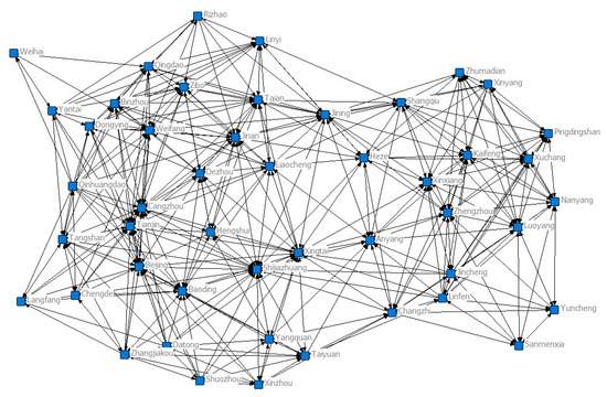
Figure 2.
Association network of PM2.5 concentration in the sampled 48 cities in 2000.
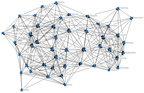
Figure 3.
Association network of PM2.5 concentration in the sampled 48 cities in 2003.
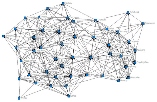
Figure 4.
Association network of PM2.5 concentration in the sampled 48 cities in 2010.
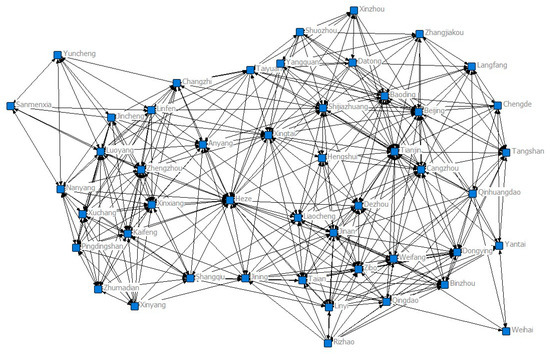
Figure 5.
Association network of PM2.5 concentration in the sampled 48 cities in 2016.
The network density of PM2.5 concentration in the 48 cities of the BTH region and its surrounding areas during 2000–2016 is shown in Table 8. The network density of each year is between 0.2429–0.2465, with an average value of 0.2442. The overall network density shows a N-shaped trend of first increasing (2000–2004), then decreasing (2004–2012), and finally increasing (2012–2016). It can be seen that the overall correlation of PM2.5 emissions in each region has slightly increased, indicating that there is linkage between PM2.5 emissions in each region. Reachability of the PM2.5 concentration correlation network was 1, indicating significant robustness of air pollution correlation among the 48 cities in the BTH region and its surrounding areas.
Table 8.
Network density of PM2.5 concentration in the sampled 48 cities.
The centrality analysis results of the top five and bottom five cities in representative years are in Table 9 and Table 10. The degree centrality illustrated the numbers of direct connections to a city. High degree indicated a city is more influential as the sources in the spatial correlation network of PM2.5 concentration and is more polluted by other cities on the spatial correlation network. The cities with top five highest degrees included Heze, Tianjin, Xingtai, Shijiazhuang, Beijing and Cangzhou, the air pollution of which were more easily directly affected by that of other cities in the network. They also showed a more significant impact on the spread of air pollution to other cities. In particular, Beijing, Tianjin and Shijiazhuang had a higher level of urbanization coupling coordination. The cities with bottom five lowest degrees included Weihai, Sanmenxia, Yuncheng, Xinzhou, Langfang and Chengde. These cities were less directly affected by air pollution from other cities and had less direct influence on air pollution transmission in the network.
Table 9.
Top five regions of degree, closeness, and betweenness centrality results in 2000, 2003, 2010 and 2016.
Table 10.
Bottom five regions of degree, closeness, and betweenness centrality results in 2000, 2003, 2010 and 2016.
The closeness centrality represented the sum of the shortcut distances between a city and other cities in the network, as it illustrated the indirect influence of a city in the network. Areas with high centrality will actively observe the PM2.5 concentration behavior of other regions and make corresponding changes in time, playing a relatively central role in the network. The top five cities in closeness included: Heze, Xingtai, Shijiazhuang, Jinan and Liaocheng, which are generally industrial zones with relatively developed economies and had the strongest indirect influence in the network. These regions have enhanced economic and industrial foundation, which can form a significant agglomeration effect. The lowest five cities in closeness included: Sanmenxia, Weihai, Yuncheng, Langfang and Zhumadian. These cities are economically underdeveloped and located at the edge of the network, which may have less indirect impact on air pollution in other cities.
The betweenness centrality measured the degree to which a certain city was located in the middle of the air pollution transmission between other two cities. These cities are functional as a “bridge”. Areas with high betweenness centrality are usually hubs connecting multiple regions, which play an important role in improving the structure of PM2.5 concentration network. Heze, Xingtai, Shijiazhuang, Liaocheng and Zhengzhou ranked the top 5 in the betweenness centrality, indicating that these cities were bridge points of other cities in the network, which is inseparable from its industrial structure and geographical location. These cities should take more responsibility for controlling the pollution level both in local and surroundings. Sanmenxia, Weihai, Yuncheng, Langfang and Zhumadian had the lowest five betweenness centrality, as air pollution transmission less passed through these cities in the network. This shows that the spatial association between these cities needs to be improved.
4. Conclusions
Based on SDM and SNA models, this paper verifies the EKC hypothesis of real GDP and PM2.5 concentration, and analyzes the impact of different driving factors on the sampled 48 cities within the BTH region and its surrounding areas during 2000–2016. In addition, the social network structure of PM2.5 concentration in the study area was also investigated. The conclusions are as follows:
- (1)
- A significant inverted U-shaped EKC with spatial spillover effect for PM2.5 concentration and economic development was shown in the sampled cities within the BTH region and its surrounding areas. The relationship between economic growth and air pollution evidenced a pattern of rising and falling after reaching the turning point of EKC. Economic growth and air pollution had significant spatial autocorrelation within the BTH region and its surrounding areas.
- (2)
- The U-shaped curve of industrial structure and air pollution presents that under the current industrial production situation, the development of secondary industry and air quality will first keep negatively and ultimately become positively related. Technological progress is beneficial for air pollution improvement, while traffic has the opposite effect. The impacts of wind, humidity, and precipitation are mostly limited to local cities, while other meteorological variables, such as temperature and humidity, show significant spillover effects.
- (3)
- Degree centrality evidenced Heze, Tianjin, Xingtai, Shijiazhuang, Beijing and Cangzhou as the most affected cities with highest degree. Closeness centrality demonstrated Heze, Xingtai, Shijiazhuang, Jinan and Liaocheng as the most central cities in the network. Between centrality proved Heze, Xingtai, Shijiazhuang, Liaocheng and Zhengzhou as the most important cities in the network. When mentioned prevention and control of PM2.5 concentration policy makers should attach more importance to the above-mentioned cities.
The policy recommendations are as follows. First, it is recommended to strengthen the air pollution prevention and supervision policies in BTH and the surrounding areas, e.g., building up regional joint prevention and control mechanisms, supervising polluting industries and upgrading the industrial structure. High-tech industrialization and service-oriented industries should be accelerated, instead of producing pollution-intensive and resource-consuming products. Second, the government should also encourage and support technological innovation in the energy conservation and environmental protection industries, which can promote air quality efficiently. Third, vehicle regulation should be implemented to control traffic pollution, such as strict vehicle emissions standards, bans on heavily polluting vehicles and vehicle restriction. Furthermore, the local government should also support non-motorized vehicle lanes and advocate clean energy vehicles to residents and extend them to small and medium sized cities.
Although this study has tried to explore empirical evidence on the existence of EKC and impacts of several indicators on air pollution from a spatial perspective, some limitations still remain to be further discussed. For instance, economic development and industry structure may also have inverse effects on air pollution as the main factors, which have not been fully discussed. Therefore, it is possible for us to adapt more comprehensive estimated methods to corporate interactive effects, which is worth exploring in further research.
Author Contributions
Conceptualization, Z.M.; Software, K.Z.; Investigation, J.L.; Data curation, H.Z.; Writing—original draft, P.H. All authors have read and agreed to the published version of the manuscript.
Funding
This research received no external funding.
Institutional Review Board Statement
Not applicable.
Informed Consent Statement
Not applicable.
Data Availability Statement
All data are available online. The data of PM2.5 concentration is from satellite data released by the Socioeconomic Data and Applications Center at Columbia University The data of nominal GDP, nominal GDP index, population at the end of the year, proportion of second industry, and annual highway passenger quantity in 2000–2016 are from the China Statistical Yearbooks (https://navi.cnki.net/KNavi/YearbookDetail?pcode=CYFD&pykm=YINFN&bh=). annual total patent grant is from Chinese Research Data Services Platform (CNRDS); annual maximum instantaneous wind speed, annual total rainy days, annual average temperature and annual average relevant humidity are from China Meteorological Science Data Center.
Conflicts of Interest
The authors declare no conflict of interest.
References
- Sasmoko, S.; Akhtar, M.Z.; Khan, H.u.R.; Sriyanto, S.; Jabor, M.K.; Rashid, A.; Zaman, K. How Do Industrial Ecology, Energy Efficiency, and Waste Recycling Technology (Circular Economy) Fit into China’s Plan to Protect the Environment? Up to Speed. Recycling 2022, 7, 83. [Google Scholar] [CrossRef]
- Liu, H.; Tian, Y.; Xu, Y.; Huang, Z.; Huang, C.; Hu, Y.; Zhang, J. Association between ambient air pollution and hospitalization for ischemic and hemorrhagic stroke in China: A multicity case-crossover study. Environ. Pollut. 2017, 230, 234–241. [Google Scholar] [CrossRef] [PubMed]
- Song, C.; Wu, L.; Xie, Y.; He, J.; Chen, X.; Wang, T.; Lin, Y.; Jin, T.; Wang, A.; Liu, Y.; et al. Air pollution in China: Status and spatiotemporal variations. Environ. Pollut. 2017, 227, 334–347. [Google Scholar] [CrossRef] [PubMed]
- Wu, Q.; Wang, R. Do Environmental Regulation and Foreign Direct Investment Drive Regional Air Pollution in China? Sustainability 2023, 15, 1567. [Google Scholar] [CrossRef]
- Fan, Q.; Yu, W.; Fan, S.; Wang, X.; Lan, J.; Zou, D.; Feng, Y.; Chan, P.W. Process analysis of a regional air pollution episode over Pearl River Delta Region, China, using the MM5-CMAQ model. J. Air Waste Manag. Assoc. 2014, 64, 406–418. [Google Scholar] [CrossRef] [PubMed]
- Jiang, C.; Wang, H.; Zhao, T.; Li, T.; Che, H. Modeling study of PM2.5 pollutant transport across cities in China’s Jing-Jin-Ji region during a severe haze episode in December 2013. Atmos. Chem. Phys. Discuss. 2015, 15, 3745–3776. [Google Scholar] [CrossRef]
- Santana, J.C.C.; Miranda, A.C.; Souza, L.; Yamamura, C.L.K.; Coelho, D.d.F.; Tambourgi, E.B.; Berssaneti, F.T.; Ho, L.L. Clean Production of Biofuel from Waste Cooking Oil to Reduce Emissions, Fuel Cost, and Respiratory Disease Hospitalizations. Sustainability 2021, 13, 9185. [Google Scholar] [CrossRef]
- Malagón-Rojas, J.N.; Parra-Barrera, E.L.; Toloza-Pérez, Y.G.; Soto, H.; Lagos, L.F.; Mendez, D.; Rico, A.; Almentero, J.E.; Quintana-Cortes, M.A.; Pinzón-Silva, D.C.; et al. Assessment of Factors Influencing Personal Exposure to Air Pollution on Main Roads in Bogota: A Mixed-Method Study. Medicina 2022, 58, 1125. [Google Scholar] [CrossRef]
- Santana, J.C.C.; Miranda, A.C.; Yamamura, C.L.K.; Silva Filho, S.C.d.; Tambourgi, E.B.; Lee Ho, L.; Berssaneti, F.T. Effects of Air Pollution on Human Health and Costs: Current Situation in São Paulo, Brazil. Sustainability 2020, 12, 4875. [Google Scholar] [CrossRef]
- Asia, C.A. China Air 2019: Air Pollution Prevention and Control Progress in Chinese Cities. Available online: http://www.allaboutair.cn/uploads/191101/China_Air_2019.rar (accessed on 26 November 2019).
- Ministry of Environmental Protection of the People’s Republic of China. Bulletin of China’s Ecological Status and Environment in 2021; Ministry of Environmental Protection of the People’s Republic of China: Beijing, China, 2022. [Google Scholar]
- Wang, Y.; Yu, H.; Li, H.; Liu, Y.; Zhao, Z.; Zhang, Y. Analysis of the impact of strengthening environmental supervision on the economy. Environ. Sustain. Dev. 2018, 43, 21–24. [Google Scholar] [CrossRef]
- Ministry of Environmental Protection of the People’s Republic of China. Record of the Regular Press Conference of the Ministry of Environmental Protection in February 2018; Ministry of Environmental Protection of the People’s Republic of China: Beijing, China, 2018. [Google Scholar]
- Peng, F.; Yu, F.; Ma, G. Analysis of social-economic benefits and environmental pollution control costs of “dispersed, disrupted and polluted” enterprises in the “2 + 26” region. Res. Environ. Sci. 2018, 31, 1993–1999. [Google Scholar]
- Grossman, G.M.; Krueger, A.B. Environmental Impacts of a North American Free Trade Agreement; National Bureau of Economic Research Working Paper Series; MIT Press: Cambridge, MA, USA, 1991. [Google Scholar]
- Kuznets, S. Economic Growth and Income Inequality. Am. Econ. Rev. 1955, 45, 1–28. [Google Scholar]
- Grossman, G.M.; Krueger, A.B. Economic Growth and the Environment. Q. J. Econ. 1995, 110, 353–377. [Google Scholar] [CrossRef]
- Selden, T.M.; Song, D. Environmental Quality and Development: Is There a Kuznets Curve for Air Pollution Emissions? J. Environ. Econ. Manag. 1994, 27, 147–162. [Google Scholar] [CrossRef]
- Apergis, N. Environmental Kuznets curves: New evidence on both panel and country-level CO2 emissions. Energy Econ. 2016, 54, 263–271. [Google Scholar] [CrossRef]
- Baležentis, T.; Streimikiene, D.; Zhang, T.; Liobikiene, G. The role of bioenergy in greenhouse gas emission reduction in EU countries: An Environmental Kuznets Curve modelling. Resour. Conserv. Recycl. 2019, 142, 225–231. [Google Scholar] [CrossRef]
- Pata, U.K. Renewable energy consumption, urbanization, financial development, income and CO2 emissions in Turkey: Testing EKC hypothesis with structural breaks. J. Clean. Prod. 2018, 187, 770–779. [Google Scholar] [CrossRef]
- Chen, Q.; Taylor, D. Economic development and pollution emissions in Singapore: Evidence in support of the Environmental Kuznets Curve hypothesis and its implications for regional sustainability. J. Clean. Prod. 2020, 243, 118637. [Google Scholar] [CrossRef]
- Dong, K.; Sun, R.; Li, H.; Liao, H. Does natural gas consumption mitigate CO2 emissions: Testing the environmental Kuznets curve hypothesis for 14 Asia-Pacific countries. Renew. Sustain. Energy Rev. 2018, 94, 419–429. [Google Scholar] [CrossRef]
- Khan, S.A.R.; Zaman, K.; Zhang, Y. The relationship between energy-resource depletion, climate change, health resources and the environmental Kuznets curve: Evidence from the panel of selected developed countries. Renew. Sustain. Energy Rev. 2016, 62, 468–477. [Google Scholar] [CrossRef]
- Churchill, S.A.; Inekwe, J.; Ivanovski, K.; Smyth, R. The Environmental Kuznets Curve in the OECD: 1870–2014. Energy Econ. 2018, 75, 389–399. [Google Scholar] [CrossRef]
- Jiang, J.-J.; Ye, B.; Zhou, N.; Zhang, X.-L. Decoupling analysis and environmental Kuznets curve modelling of provincial-level CO2 emissions and economic growth in China: A case study. J. Clean. Prod. 2019, 212, 1242–1255. [Google Scholar] [CrossRef]
- Li, T.; Wang, Y.; Zhao, D. Environmental Kuznets Curve in China: New evidence from dynamic panel analysis. Energy Policy 2016, 91, 138–147. [Google Scholar] [CrossRef]
- Diao, X.D.; Zeng, S.X.; Tam, C.M.; Tam, V.W.Y. EKC analysis for studying economic growth and environmental quality: A case study in China. J. Clean. Prod. 2009, 17, 541–548. [Google Scholar] [CrossRef]
- Fujii, H.; Iwata, K.; Chapman, A.; Kagawa, S.; Managi, S. An analysis of urban environmental Kuznets curve of CO2 emissions: Empirical analysis of 276 global metropolitan areas. Appl. Energy 2018, 228, 1561–1568. [Google Scholar] [CrossRef]
- Wang, Y.; Han, R.; Kubota, J. Is there an Environmental Kuznets Curve for SO2 emissions? A semi-parametric panel data analysis for China. Renew. Sustain. Energy Rev. 2016, 54, 1182–1188. [Google Scholar] [CrossRef]
- Zhou, C.; Wang, S.; Wang, J. Examining the influences of urbanization on carbon dioxide emissions in the Yangtze River Delta, China: Kuznets curve relationship. Sci. Total Environ. 2019, 675, 472–482. [Google Scholar] [CrossRef]
- Wang, S.; Liu, X. China’s city-level energy-related CO2 emissions: Spatiotemporal patterns and driving forces. Appl. Energy 2017, 200, 204–214. [Google Scholar] [CrossRef]
- Apergis, N.; Christou, C.; Gupta, R. Are there Environmental Kuznets Curves for US state-level CO2 emissions? Renew. Sustain. Energy Rev. 2017, 69, 551–558. [Google Scholar] [CrossRef]
- Azam, M.; Khan, A.Q. Testing the Environmental Kuznets Curve hypothesis: A comparative empirical study for low, lower middle, upper middle and high income countries. Renew. Sustain. Energy Rev. 2016, 63, 556–567. [Google Scholar] [CrossRef]
- Pablo-Romero, M.d.P.; De Jesús, J. Economic growth and energy consumption: The Energy-Environmental Kuznets Curve for Latin America and the Caribbean. Renew. Sustain. Energy Rev. 2016, 60, 1343–1350. [Google Scholar] [CrossRef]
- Bölük, G.; Mert, M. The renewable energy, growth and environmental Kuznets curve in Turkey: An ARDL approach. Renew. Sustain. Energy Rev. 2015, 52, 587–595. [Google Scholar] [CrossRef]
- Park, S.; Lee, Y. Regional model of EKC for air pollution: Evidence from the Republic of Korea. Energy Policy 2011, 39, 5840–5849. [Google Scholar] [CrossRef]
- Orubu, C.O.; Omotor, D.G. Environmental quality and economic growth: Searching for environmental Kuznets curves for air and water pollutants in Africa. Energy Policy 2011, 39, 4178–4188. [Google Scholar] [CrossRef]
- Hossain, M.R.; Rej, S.; Awan, A.; Bandyopadhyay, A.; Islam, M.S.; Das, N.; Hossain, M.E. Natural resource dependency and environmental sustainability under N-shaped EKC: The curious case of India. Resour. Policy 2023, 80, 103150. [Google Scholar] [CrossRef]
- Wang, Q.; Yang, T.; Li, R. Does income inequality reshape the environmental Kuznets curve (EKC) hypothesis? A nonlinear panel data analysis. Environ. Res. 2023, 216, 114575. [Google Scholar] [CrossRef]
- Jahanger, A.; Yu, Y.; Hossain, M.R.; Murshed, M.; Balsalobre-Lorente, D.; Khan, U. Going away or going green in NAFTA nations? Linking natural resources, energy utilization, and environmental sustainability through the lens of the EKC hypothesis. Resour. Policy 2022, 79, 103091. [Google Scholar] [CrossRef]
- Tenaw, D.; Beyene, A.D. Environmental sustainability and economic development in sub-Saharan Africa: A modified EKC hypothesis. Renew. Sustain. Energy Rev. 2021, 143, 110897. [Google Scholar] [CrossRef]
- Özokcu, S.; Özdemir, Ö. Economic growth, energy, and environmental Kuznets curve. Renew. Sustain. Energy Rev. 2017, 72, 639–647. [Google Scholar] [CrossRef]
- Qin, M.; Wang, X.; Hu, Y.; Huang, X.; He, L.; Zhong, L.; Song, Y.; Hu, M.; Zhang, Y. Formation of particulate sulfate and nitrate over the Pearl River Delta in the fall: Diagnostic analysis using the Community Multiscale Air Quality model. Atmos. Environ. 2015, 112, 81–89. [Google Scholar] [CrossRef]
- Hao, Y.; Liu, Y.; Weng, J.-H.; Gao, Y. Does the Environmental Kuznets Curve for coal consumption in China exist? New evidence from spatial econometric analysis. Energy 2016, 114, 1214–1223. [Google Scholar] [CrossRef]
- Kennedy, P.; Hutchinson, E. The relationship between emissions and income growth for a transboundary pollutant. Resour. Energy Econ. 2014, 38, 221–242. [Google Scholar] [CrossRef]
- Maddison, D. Environmental Kuznets curves: A spatial econometric approach. J. Environ. Econ. Manag. 2006, 51, 218–230. [Google Scholar] [CrossRef]
- Ding, Y.; Zhang, M.; Chen, S.; Wang, W.; Nie, R. The environmental Kuznets curve for PM2.5 pollution in Beijing-Tianjin-Hebei region of China: A spatial panel data approach. J. Clean. Prod. 2019, 220, 984–994. [Google Scholar] [CrossRef]
- Balado-Naves, R.; Baños-Pino, J.F.; Mayor, M. Do countries influence neighbouring pollution? A spatial analysis of the EKC for CO2 emissions. Energy Policy 2018, 123, 266–279. [Google Scholar] [CrossRef]
- Xie, Q.; Xu, X.; Liu, X. Is there an EKC between economic growth and smog pollution in China? New evidence from semiparametric spatial autoregressive models. J. Clean. Prod. 2019, 220, 873–883. [Google Scholar] [CrossRef]
- Huang, J.; Chen, X.; Huang, B.; Yang, X. Economic and environmental impacts of foreign direct investment in China: A spatial spillover analysis. China Econ. Rev. 2017, 45, 289–309. [Google Scholar] [CrossRef]
- Li, B.; Wu, S. Effects of local and civil environmental regulation on green total factor productivity in China: A spatial Durbin econometric analysis. J. Clean. Prod. 2017, 153, 342–353. [Google Scholar] [CrossRef]
- Liu, X.; Sun, T.; Feng, Q. Dynamic spatial spillover effect of urbanization on environmental pollution in China considering the inertia characteristics of environmental pollution. Sustain. Cities Soc. 2020, 53, 101903. [Google Scholar] [CrossRef]
- Du, Y.; Wan, Q.; Liu, H.; Liu, H.; Kapsar, K.; Peng, J. How does urbanization influence PM_2.5 concentrations? Perspective of spillover effect of multi-dimensional urbanization impact. J. Clean. Prod. 2019, 220, 974–983. [Google Scholar] [CrossRef]
- Zhu, L.; Gan, Q.; Liu, Y.; Yan, Z. The impact of foreign direct investment on SO2 emissions in the Beijing-Tianjin-Hebei region: A spatial econometric analysis. J. Clean. Prod. 2017, 166, 189–196. [Google Scholar] [CrossRef]
- Du, Y.; Sun, T.; Peng, J.; Fang, K.; Liu, Y.; Yang, Y.; Wang, Y. Direct and spillover effects of urbanization on PM_2.5 concentrations in China’s top three urban agglomerations. J. Clean. Prod. 2018, 190, 72–83. [Google Scholar] [CrossRef]
- Yang, T.; Zhou, K.; Ding, T. Air pollution impacts on public health: Evidence from 110 cities in Yangtze River Economic Belt of China. Sci. Total Environ. 2022, 851, 158125. [Google Scholar] [CrossRef]
- Jiang, W.; Gao, W.; Gao, X.; Ma, M.; Zhou, M.; Du, K.; Ma, X. Spatio-temporal heterogeneity of air pollution and its key influencing factors in the Yellow River Economic Belt of China from 2014 to 2019. J. Environ. Manag. 2021, 296, 113172. [Google Scholar] [CrossRef]
- Wang, H.; Gu, K.; Sun, H.; Xiao, H. Reconfirmation of the symbiosis on carbon emissions and air pollution: A spatial spillover perspective. Sci. Total Environ. 2023, 858, 159906. [Google Scholar] [CrossRef]
- Zhao, C.; Wang, B. How does new-type urbanization affect air pollution? Empirical evidence based on spatial spillover effect and spatial Durbin model. Environ. Int. 2022, 165, 107304. [Google Scholar] [CrossRef] [PubMed]
- Wang, S.; Fang, C.; Wang, Y. Spatiotemporal variations of energy-related CO2 emissions in China and its influencing factors: An empirical analysis based on provincial panel data. Renew. Sustain. Energy Rev. 2016, 55, 505–515. [Google Scholar] [CrossRef]
- He, Y.; Lai, Z.; Liao, N. Evaluating the effect of low-carbon city pilot policy on urban PM2.5: Evidence from a quasi-natural experiment in China. Environ. Dev. Sustain. 2023, 1–27. [Google Scholar] [CrossRef]
- Yang, L.; Qin, C.; Li, K.; Deng, C.; Liu, Y. Quantifying the Spatiotemporal Heterogeneity of PM2. 5 Pollution and Its Determinants in 273 Cities in China. Int. J. Environ. Res. Public Health 2023, 20, 1183. [Google Scholar] [CrossRef] [PubMed]
- Jia, W.; Li, L.; Lei, Y.; Wu, S. Synergistic effect of CO2 and PM2.5 emissions from coal consumption and the impacts on health effects. J. Environ. Manag. 2023, 325, 116535. [Google Scholar] [CrossRef] [PubMed]
- Es’haghi, S.R.; Karamidehkordi, E. Understanding the structure of stakeholders−projects network in endangered lakes restoration programs using social network analysis. Environ. Sci. Policy 2023, 140, 172–188. [Google Scholar] [CrossRef]
- Wang, H.; Ge, Q. Analysis of the Spatial Association Network of PM2.5 and Its Influencing Factors in China. Int. J. Environ. Res. Public Health 2022, 19, 12753. [Google Scholar] [CrossRef] [PubMed]
- Yan, D.; Lei, Y.; Shi, Y.; Zhu, Q.; Li, L.; Zhang, Z. Evolution of the spatiotemporal pattern of PM2.5 concentrations in China—A case study from the Beijing-Tianjin-Hebei region. Atmos. Environ. 2018, 183, 225–233. [Google Scholar] [CrossRef]
- Li, M.; Mao, C. Spatial Effect of Industrial Energy Consumption Structure and Transportation on Haze Pollution in Beijing-Tianjin-Hebei Region. Int. J. Environ. Res. Public Health 2020, 17, 5610. [Google Scholar] [CrossRef] [PubMed]
- Ma, Y.; Zhang, W.; Zhang, L.; Gu, X.; Yu, T. Estimation of Ground-Level PM2.5 Concentration at Night in Beijing-Tianjin-Hebei Region with NPP/VIIRS Day/Night Band. Remote Sens. 2023, 15, 825. [Google Scholar] [CrossRef]
- Liu, N.; Li, S.; Zhang, F. Multi-Scale Spatiotemporal Variations and Drivers of PM2.5 in Beijing-Tianjin-Hebei from 2015 to 2020. Atmosphere 2022, 13, 1993. [Google Scholar] [CrossRef]
- Zhao, X.; Zhou, W.; Han, L.; Locke, D. Spatiotemporal variation in PM2.5 concentrations and their relationship with socioeconomic factors in China’s major cities. Environ. Int. 2019, 133, 105145. [Google Scholar] [CrossRef]
- Mao, X.; Wang, L.; Pan, X.; Zhang, M.; Wu, X.; Zhang, W. A study on the dynamic spatial spillover effect of urban form on PM2.5 concentration at county scale in China. Atmos. Res. 2022, 269, 106046. [Google Scholar] [CrossRef]


Disclaimer/Publisher’s Note: The statements, opinions and data contained in all publications are solely those of the individual author(s) and contributor(s) and not of MDPI and/or the editor(s). MDPI and/or the editor(s) disclaim responsibility for any injury to people or property resulting from any ideas, methods, instructions or products referred to in the content. |
© 2023 by the authors. Licensee MDPI, Basel, Switzerland. This article is an open access article distributed under the terms and conditions of the Creative Commons Attribution (CC BY) license (https://creativecommons.org/licenses/by/4.0/).