1. Introduction
Per 2019 statistics, the agricultural segment contributes a significant 7.1%, or an estimated MYR 101.5 billion, to the Malaysian national gross domestic product (GDP) economic pie. The top major value-added contributors were oil palm at 37.7%, followed by agriculture at 25.9%, livestock at 15.3%, fishing at 12.0%, forestry & logging at 6.3%, and rubber at 3.0% [
1,
2]. Reference evapotranspiration uncertainties are a key part of the knowledge base for sustainable water resource management. Meanwhile, evapotranspiration (ET) is a key part of the hydrological cycle that influences farm irrigation scheduling, crop water resource management, changing climate conditions, and environmental assessment. Furthermore, in arid and semi-arid regions where water resources are scarce, evapotranspiration becomes an essential criterion in decision-making regarding water exploitation [
3,
4,
5,
6]. Evapotranspiration occurs when water evaporates from the soil and crop surfaces into the atmosphere. From the volume of water demand, the farmer can determine whether to irrigate their plants and customize their irrigation practices [
7,
8,
9]. Over-irrigation leads to rotting roots and leaching of nitrogen and micronutrients, while water scarcity causes vital nutrients to not travel through the plant [
10,
11]. Hence, agricultural surplus and water shortage can affect overall crop growth, development, yield, and quality [
12,
13]. Meanwhile, transpiration is induced by the chemical and biological changes that occur in a plant when it undergoes photosynthesis and converts carbon dioxide to oxygen [
14,
15].
Accurate prediction of reference evapotranspiration () is vital in comprehending water demands from the plant, impacting water resource management and irrigation systems scheduling. Prediction of evapotranspiration rate enables the estimation of crop water demand. Accurate measurement of crop water needs forecasts of reference evapotranspiration. The lack of meteorological data in weather stations causes increased difficulties in calculating reference evapotranspiration using the Penman–Montieth 56 equation. Meteorological variables impact evapotranspiration. Recent research studies proposed solutions based on the Penman–Montieth empirical formula and machine learning model in reference to evapotranspiration forecasting. Hence, it is difficult to obtain a single formula with all relevant climate variables described. Therefore, machine learning models are alternatives to conventional techniques because of their superior ability to solve issues that exhibit non-linearity and complexity. Machine learning models can readily use the empirical equation with reduced climate variables, as they are more straightforward.
In order to determine the reference evapotranspiration based on changes in climate variables, the aim of this paper is to build a model capable of collecting local climate data and running forecasts in situ to improve accuracy. Recent advances in the processing capacity of an embedded system like Raspberry Pi create the opportunity to build low-cost local forecast models with impressive computing power. This paper also first trains and selects a vector autoregression (VAR) forecast model based on public weather data and then integrates weather data acquisition capability in an embedded system using a Raspberry Pi and sensors for future forecast model enhancement.
The research presented in the paper is considered novel research since it proposes a new and innovative approach to improve the forecasting of reference evapotranspiration (), a critical standard measurement for environmental parameters that affect water management for agriculture, using the vector autoregression (VAR) model. It has been determined that this method has not been attempted before in the research literature using 20-year, 1-year, and 2-month datasets with comparative analysis of the Granger causality test, cointegration test, Johansen test, unit root test, and augmented Dickey–Fuller (ADF) test.
The rest of this paper is organized as follows.
Section 2 reviews some relevant studies.
Section 3 provides the description of evapotranspiration, embedded systems, and forecast results with historical data.
Section 4 introduces the methodology of the VAR-based model.
Section 5 provides the results and discussion of the VAR-based model. Lastly,
Section 6 concludes this work.
2. State of the Art
2.1. Penman–Montieth Empirical Formula
Complete meteorological data required by the FAO-56 PM equation are not commonly available due to limitations in data acquisition [
16]. Hence, the analysis was performed by researchers in production and assessment using reduced data requirements in empirical equations. The study suggested alternate methods for estimating meteorological data in empirical equations without sunlight, ambient humidity, and wind speed data. Empirical equations with reduced meteorological variables yield unsatisfactory results [
17]. It shows an inconsistent performance for the research location’s climatic conditions where the model is deployed, although it requires fewer data. Temperature-based empirical models are fundamental out of the various reduced meteorological empirical equations, as almost all weather stations frequently collect temperature, and temperature-based models are widely used [
18]. Research has shown estimation of reference evapotranspiration with relative humidity, as additional input yields superior performances at lower extra cost, and a comparatively smaller budget to set up an ambient humidity sensor on a weather station compared to other sensors. Additionally, portable hybrid thermo-hygrometers that can collect temperature and ambient humidity can be considered given their low cost [
19]. Regarding the use of empirical models to calculate the FAO-56 PM equation, there is a lack of research in finding a causal relationship between climate variables and evapotranspiration under various scenarios [
20]. A simplified version of the Penman–Montieth equation using a single dependent climate variable or a lesser climate variable combo than the FAO-56 PM equation was found in other research. Forecasting methods such as Hargreaves–Samani and the modified daily Thornthwaite equation are used instead of the FAO-56 PM equation due to the lack of climate data collection from the environment. However, research lacks evidence on climate variable weighting on evapotranspiration, and the causal effect of the selected climate variable is not transparent to the user.
2.2. Machine Learning Model Performance
Recent research shows low utilization of support vector machines (SVM) and artificial neural networks (ANN) in reference evapotranspiration forecasting. The ANN model shows better performance compared to traditional methods in these studies. Similarly, SVM has also shown strong results in reference evapotranspiration estimations [
21]. Reference evapotranspiration exhibits non-linearity, non-static, and complex behavior [
22].
2.2.1. Artificial Neural Network (ANN) Performance
Extensive research has been done in estimating reference evapotranspiration using the artificial neural network (ANN) model. The prediction results showed the best work when all climate variables are considered in the calculation. The ANN model shows high accuracy in predicting the non-linearity of evapotranspiration.
For the estimation of (
) in Brazil, support vector machine and artificial neural networks were used in accessing empirical equations. K-means have been deployed to identify meteorological stations with the same weather features. Historical climate data were used as an extra input for a predictive ML model. The performance boost was given by clustering, and previous results were observed. The best result was from the artificial neural network with meteorological data from past days [
23].
For crop evapotranspiration estimation, k-nearest neighbor (k-NN), ANN, and adaptive boosting (AdaBoost) machine learning models were tested. Four meteorological input data scenarios were checked for performance. For the first time, k-NN and AdaBoost were applied to estimate crop evapotranspiration. With limited meteorological data, the k-NN model performed better than other models. With a complete range of meteorological inputs, the ANN model produced the best results [
24].
2.2.2. Extreme Learning Machine (ELM) Performance
Similarly, for the extreme learning machine (ELM), research has been done to estimate reference evapotranspiration and compared it to the artificial neural network (ANN) model. The prediction result shows the ELM model generates better results compared to ANN and GRNN models when the () empirical formula of only one climate variable is used.
ELM was used to measure daily (
) using temperature data only. Extreme machine for learning (ELM), GRNN (generalized regression neural network), and Hargreaves developed and calibrated evaluated local and pooled data management scenarios. ELM worked better for local scenarios than GRNN, Hargreaves, and Hargreaves calibrated. Among the considered models for pooled scenarios, GRNN provided the most detailed results [
25].
In modeling (
), the capacity of four separate data-driven models is evaluated. The data-driven models were better than the empirical models for (
) prediction. Using PSO to optimize ELM could boost ELM model efficiency. PSO–ELM gave the best accuracy of the (
) prediction [
26].
2.2.3. Support Vector Machine (SVM) Performance
The research found that SVM modeling in estimating reference evapotranspiration produced better results than the ANN model using an empirical formula. Enhanced SVN models such as SVN–WOA (whale optimization algorithm) and least square support vector machine (LSSVM) yield better performance than using SVN solely. The LSSVM model shows high accuracy, efficiency, and generalization performance in predicting evapotranspiration.
In this research, three distinct models of evapotranspiration were compared by [
27]. The models are different based on the input variables. Four variants of each model were applied: M5P regression tree, bagging, random forest, and support vector machine.
DL models yield outstanding performance outside study areas in forecasting reference evapotranspiration. Deep neural networks (DNN), long short-term memory neural networks (LSTM), and temporal convolution neural networks (TCN) have been trained for comparison. The forecasting result of the TCN has greatly surpassed empirical equations. This research’s empirical equations include two temperature-dependent models: Hargreaves (H) and Hargreaves (MH) modified. The three radiation-dependent models are Ritchie (R), Priestley–Taylor (P), and Makkink (M). Two analytical humidity-dependent models, Romanenko (ROM) and Schendel (S), are tested with R2 and RMSE as validation of the model. The use of the T-test method is the suggested models’ efficiency assessment. TCN outperformed support vector machine (SVM) and random forest (RF) models [
28].
At the three stations in Iran, daily reference evapotranspiration was modeled. Ambient temperature, ambient humidity, sunlight duration, and wind speed were model inputs. For optimal input recognition, pre-processing was used, proposed by an approach to the whale optimization algorithm promoting vector regression (SVR) by couples. Model performance assessment was completed by running analyses with root mean square error (RMSE), normalized RMSE, mean absolute error (MAE), determination coefficient (R2), and Nash–Sutcliffe efficiency (E). The optimized whale algorithm for support vector regression performed better than the sole support vector regression (SVN). Artificial intelligence (AI) was used to combat (
) non-linearity [
29].
2.2.4. Gene Expression Programming (GEP) Performance
The gene expression programming model was used and compared to other machine learning models. Overall, the GEP model shows worse performance than ANN, SVM, and MARS in predicting generalized reference evapotranspiration.
The mean evapotranspiration collected monthly is compared and calculated in Iran. This research assesses the performance of MARS, SVM, GEP, and empirical equations for the forecasting of evapotranspiration. The model’s MARS and SVM–RBF outperformed GEP and SVM. The most precise scenario is MARS16 (Rs, T, RH, u2) [
30].
In [
31], 8 GEP models were compared to 8 ANN models to estimate the (
) result of GEP, which was shown to be slightly worse than the ANN model. Calibrated reference evapotranspiration ((
), cal) was used. Climatic data from 19 meteorological stations from 1980–2010 (30 years) was used for Saudi Arabia.
Ref. [
32] uses data from the same station to construct the ML model. The random forest algorithm was used in the modeling of (
). The result was compared with the gene expression programming (GEP) model. Model validation consists of the coefficient of determination (R2), Nash–Sutcliffe coefficiencies of efficiency (NSCE), the root mean squared error (RMSE), and percent bias (PBIAS).
2.2.5. Autoregression (AR) Performance
The autoregression model was used to predict short-term weather forecasts, which predict current and future values based on historical climate variables in time series. The AR model is more straightforward than other machine learning methodologies but results in non-linearity of long-term weather trends.
Ref. [
33] utilized the univariate autoregression model (AR) and moving average models (MA) separately in his first attempt. The author then integrated moving averages and autoregressive models to build an autoregressive integrated moving average (ARIMA) model. The historical climate variables were used in these models to create forecasts, but a univariate model such as AR and MA lack of data can be used for other time series.
2.2.6. Deep Learning Performance
Bedi Jatin [
34] presented three models based on deep learning to forecast evapotranspiration. Using only the most basic of previously collected evapotranspiration data, a baseline model based on a moving window is proposed for use in subsequent forecasts. The proposed model uses the long short-term memory network (LSTMN) model to aid in the management of historical data dependencies. The prediction performance of the initial model is then enhanced by introducing/extending the concept of transfer learning.
2.2.7. Adaptive Neuro-Fuzzy Inference System (ANFIS)
Aghelpour et al. [
35] compared the accuracy of various stochastic and machine learning models for predicting (
) in the province of Mazandaran, Iran. These models include the autoregressive (AR), moving average (MA), autoregressive moving average (ARMA), and autoregressive integrated moving average (ARIMA) techniques, as well as the least squares support vector machine (LSSVM), adaptive neuro-fuzzy inference system (ANFIS), and generalized regression neural network (GRNN). Five synoptic stations in the province of Mazandaran provided the data used in this analysis. Air temperature (low, high, and average), humidity (low, high, and average), wind speed, and sunshine hours are all included. The Iranian Meteorological Organization has regularly sent these updates from 2003 to the present. (
) rates for each day are then calculated using these factors and the FAO-56 Penman–Monteith model.
2.2.8. Auto Encoder-Decoder Bidirectional LSTM
For the first time [
36], a powerful deep learning model, auto encoder-decoder bidirectional long short-term memory (AED-BiLSTM), was used to predict weekly (
) 1–3 weeks in advance. The climates of Kermanshah (which is semi-arid), Nowshahr (which is very humid), and Yazd (which is arid) were studied and compared. A statistical window of 20 years (2000–2019) was used, with the first 15 years (2000–2014) used for model training and the last five years (2015–2019) used for model testing.
2.3. Critical Analysis
With regard to calculating () for reference evapotranspiration, comparative analysis shows certain drawbacks to using existing approaches. The Penman–Montieth approach requires a large amount of meteorological data, which may be difficult to obtain in some regions. As for the machine learning model, it may not be able to model the underlying physics of the system accurately.
Artificial neural network (ANN) also requires a large amount of data and computational resources to train, similar to the Penman–Montieth method, and may be prone to overfitting. Extreme learning machine’s (ELM) disadvantages may be due to the fact that it is not able to capture the complex relationships in the data. The same applies to support vector machine (SVM), as it may not be well-suited for high-dimensional data.
Analysis of gene expression programming (GEP) demonstrates that it may be computationally expensive and potentially not able to converge to a solution. As for the autoregression (AR) method, it is potentially unable to capture non-linear relationships in the data.
The weaknesses of the deep learning technique include the large amount of data and considerable computational resources required to train it, and that it may be prone to overfitting. The adaptive neuro-fuzzy inference system (ANFIS) algorithm is also potentially unable to handle non-linear and non-stationary data. To sum up, the auto encoder-decoder bidirectional LSTM technique may require a large amount of data and computational resources to train and may be prone to overfitting.
For the earlier studies, comparative analysis was made with the Granger causality test, cointegration test, Johansen test, unit root test, and augmented Dickey–Fuller (ADF) test. Based on the results, further work is needed to improve the accuracy using neural networks, a potential method that uses a different approach. The anticipated drawback of the neural network method is the tremendous resources required to build the model as well as being computationally-intensive to train the dataset to improve the accuracy. One issue that needs to be resolved is identifying workaround methods to build and train neural network models using many fewer resources. The paper does not apply the SVM method in the research but simply includes it for comparative analysis for literature review.
The vector autoregression (VAR) model is superior than other techniques introduced in the paper since: (I) multiple clear evaluation metrics, such as mean absolute percentage error (MAPE), margin of error (ME), mean absolute error (MAE), mean percentage error (MPE), root mean squared error (RMSE), correlation coefficient (CORR), and min–max have been used to evaluate the accuracy of the forecast data and have been shown to be more accurate than other methods; (II) the data were split into 80% training data and 20% validation datasets to ensure that the models are adequately trained and tested on independent data, leading to a more accurate evaluation of the model performance; and (III) when the datasets mentioned above were used to train and evaluate both the VAR model’s and other techniques’ performance using the evaluation metric defined in (I) above, the results showed that the VAR model performs better.
4. Materials and Methods
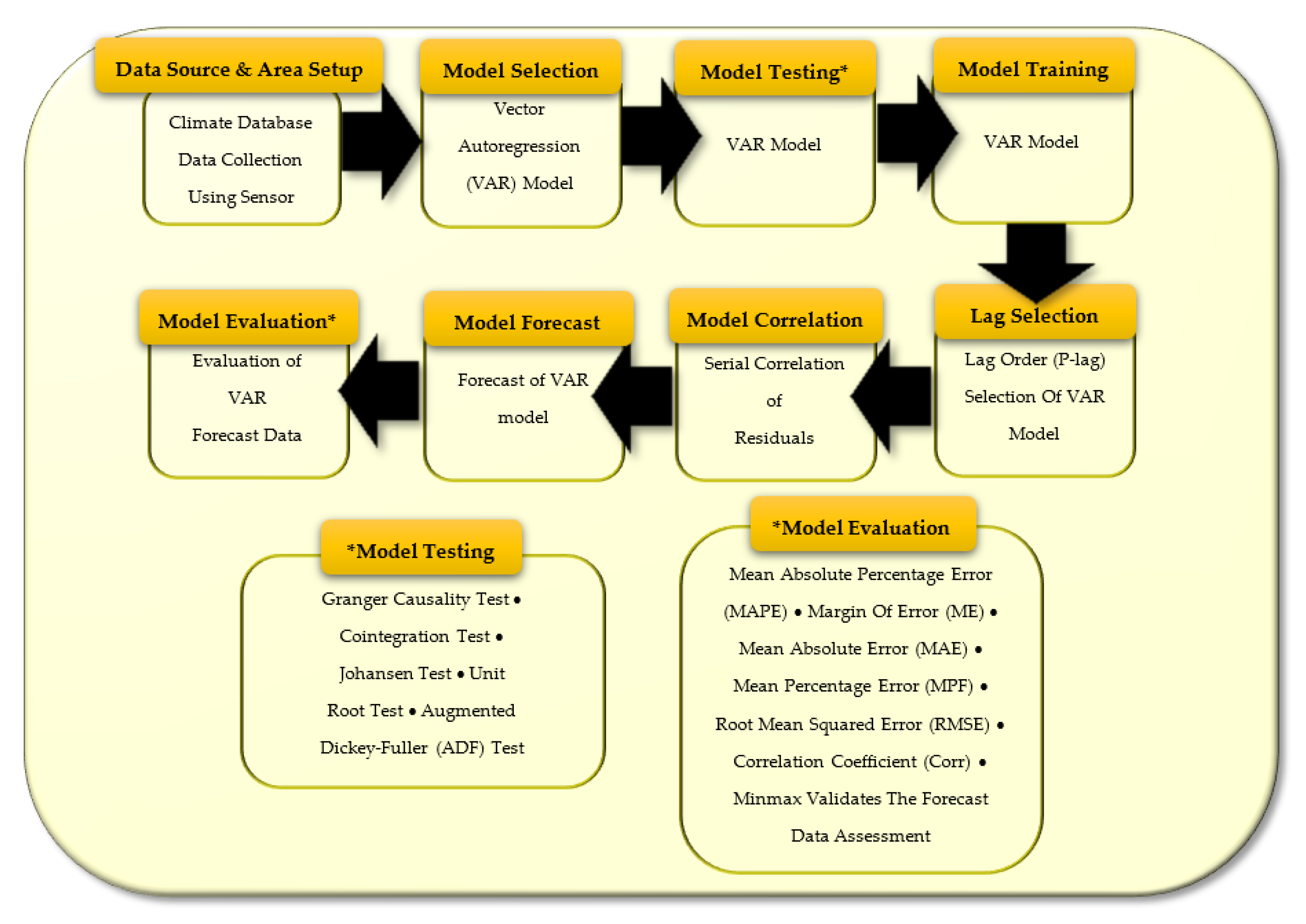
As shown in
Figure 1, the steps of the methodology of this paper are provided. These steps are described as follows.
4.1. Climate Database and Study Area
The study area is based in Penang, Malaysia. The weather data are calculated based on NMM (nonhydrostatic meso-scale modelling) or NEMS (NOAA Environment Monitoring System) technology from meteoblue forecasts, allowing for extensive information on topography, land cover, and surface cover. Official and reliable weather station data based on National Hydrological Network Management System (SPRHiN) are scarce in Penang. The SPRHiN weather database reported zero evapotranspiration measurement stations on Penang Island. Most of the weather station measurements are useful only for a 3- to 12-km radius surrounding the station. Weather stations are located unevenly on land surfaces, with only a few places with weather stations in the vicinity. In most areas, stations are widely spaced or without any weather station in the vicinity. The meteoblue database covers the spatial resolution of a 3- to 30-km square grid, which is suitable for regional prediction of evapotranspiration compared to less than 1 km coverage in the localized weather station. It provides 100% consistency and completeness of data. The mean daily meteorological variables collected include the mean temperature 2 m above ground (T), relative humidity 2 m above ground (RH), wind speed 10 m above ground (WS), sunshine duration in minutes (SD), pressure above sea level (P), and reference evapotranspiration (
) [
47].
Climate datasets with time series are split into 80% training data and 20% test data. Forecast data will be compared against the actual test data. After the VAR model is built, local climate data will be acquired by the DHT11 temperature sensor for future model enhancement.
With respect to constrained research timeline, with the use of 20-year and 1-year public domain datasets to comprehend long-term seasonal variations, and with the 2-month (November 2020 to January 2021 timeline) dataset to explain transient climate changes, it should be sufficient to establish an accurate prediction of general reference evapotranspiration using the vector autoregression model for such a geographically-focsued location as Penang, Malaysia.
4.2. Vector Autoregression (VAR) Model
The model of vector autoregression (VAR) is a multivariate forecasting algorithm. It is used when two or more time series variables are affecting each another. Each variable is modeled as a function of its past value, or time-delayed series value, considered by the autoregression model [
48]. The VAR terminology involves the generalization of the univariate autoregression model to a vector of variables. The VAR model is a stochastic process that, as a linear function of its past values and the past values of all other variables in the group, represents time-dependent variables. Thus, the VAR model is formed as an equation of stochastic differences. In general, an autoregression model is a linear time series equation with a set of lag values combined. The set of lag values in the time series is used to predict the current value and future value.
In a typical autoregression model, the AR
p equation is denoted as in Equation (
1), where
is the intercept or constant and
is the coefficients of lag from
t−1 to
p. Order
p is the
p-lag value of
Y, and they are the predictors in the equation. The error term is
[
49]. Vector autoregression (VAR) is the main element and particular case of the moving average (MA) model, including the autoregression integrated moving average (ARIMA) and the autoregression moving average (ARMA) time series models. The vector autoregression model has a more complex stochastic structure. The vector autoregression model (VAR) consists of an equation of two or more interlocking equations of stochastic difference, which contains two or more evolving random variables. VAR, AR, ARMA, and ARIMA algorithms are similar in that they require a series of observations to train the model before using the model for forecasting. However, the difference between VAR and the rest of the algorithms is that VAR is suitable for multivariate data, whereas AR, ARMA, and ARIMA are univariate models. The linear regressive variable
Y is affected by its past value or predictors, but not the other way around. On the contrary, VAR is bidirectional, and its variables affect each other [
50].
The reason for not using multiple linear regressions is that it does not specifically consider time series data, which refer to data collected over time. Multiple linear regression statistical techniques are also ideal for modeling linear relationships between a set of independent variables and a dependent variable. The proposed VAR model considers the time series data in the model.
The adaptive learning rate is a technique used in machine learning to adjust the learning rate during training to improve the performance of the model. It is commonly used in optimization algorithms such as gradient descent and its variants to help the model converge to a better solution.
In the case of a VAR model, the parameters of the model are typically estimated using maximum likelihood estimation (MLE) or a related method, which do not rely on gradient-based optimization. Therefore, the concept of an adaptive learning rate is not directly applicable to the estimation of VAR models.
4.3. Various Tests
Conducting several tests like the Granger causality test, cointegration test, Johansen test, unit root test, and augmented Dickey–Fuller (ADF) test on a vector autoregression (VAR) model can help validate the VAR method by assessing different aspects of the model:
Granger causality test: This test is used to determine whether one time series is useful in forecasting another time series. It can be used to determine if there is a causal relationship between the variables in the VAR model and if the model is correctly specified.
Cointegration test: This test is used to determine if there is a long-term relationship between the variables in the VAR model. It can be used to confirm that the variables in the VAR model are cointegrated and that the model is correctly specified.
Johansen test: This test is used to determine the number of cointegrating relationships between the variables in the VAR model. It can be used to confirm that the variables in the VAR model are cointegrated and that the model is correctly specified.
Unit root test: This test is used to determine whether the variables in the VAR model are non-stationary or stationary. It can be used to confirm that the variables in the VAR model are stationary and that the model is correctly specified.
Augmented Dickey–Fuller (ADF) test: This test is used to determine whether a time series has a unit root or not. It can be used to confirm that the variables in the VAR model are stationary and that the model is correctly specified.
By conducting these tests, the researcher can ensure that the VAR method is correctly specified and that the variables in the model are cointegrated, stationary, and have a causal relationship. This can increase the confidence in the forecasting results generated by the VAR model.
Granger causality test:
The null hypothesis in a Granger causality test is that the past values of one time series (X) do not have any significant information for predicting the future values of another time series (Y), beyond what can be already predicted by the past values of Y alone. This can be stated mathematically as H0: x = 0, where x represents the coefficients of the lagged values of X in the forecasting equation for Y. The null hypothesis is that these coefficients are equal to zero, indicating that past values of X do not contain any additional information for predicting future values of Y.
Alternatively, the null hypothesis can also be stated as H0: X does not Granger cause Y. This means that the past values of X do not have a causal effect on the future values of Y.
It is worth noting that if the null hypothesis is rejected in a Granger causality test, it does not necessarily mean that there is a causal relationship between the two time series, but only that the past values of one series contain additional information that can be used to predict the future values of the other series. If the probability value is less than any
level, then the hypothesis would be rejected at that level. Stationary time series perform the Granger causality test with two or more variables. Non-stationary time series perform the test using differences with some lags, which are chosen based on information criteria, such as Akaike information criterion (AIC), Bayesian information criterion (BIC), Akaike’s final prediction error (FPE), or Hannan–Quinn information criterion (HQIC) [
51]. The null Granger causality hypothesis is dismissed if a regression with a significance level of 0.05 has not maintained any lagged values or
p-values of an explanatory variable.
Cointegration Test: The cointegration test is used to assess if there is a long-term statistical association between many time series. The cointegration test analyzes two of the non-stationary time series, namely, variance and means that vary over time, which allows long-term parameter estimation or equilibrium in the unit root variables method. If a linear combination of such variables has a lower integration order, two sets of variables are cointegrated. Integration order (d) is the number of differences appropriate for converting non-stationary time series into stationary time series. The basic principle on which the model of vector autoregression (VAR) is based is the cointegration test. Several tests, including the Engle–Granger test, the Phillips–Ouliaris test, and the Johansen test, can be used to detect the cointegration of variables. Johansen’s test was used in this situation [
52].
Johansen Test: The Johansen test is used to test the cointegration of a few different non-stationary time series data relationships. The Johansen test is an improvement over the Engle–Granger test, facilitating the cointegration of more than one relationship. It removes the issue of choosing a dependent variable and the problems caused by errors from one point to the next. As such, the test can distinguish many cointegrating vectors. Due to unreliable output results with restricted sample size, the Johansen test is vulnerable to asymptotic or large sample size properties. The Johansen test has two main types: trace and maximum eigenvalue tests. The trace test determines the combination number of linearity in time series results. The null hypothesis is set to zero; using the trace test to test for cointegration in a sample, it tests whether the null hypothesis is denied. If it is denied, it can be concluded that the analysis has a cointegration relationship. Therefore, the null hypothesis should be discounted to justify a cointegration relationship in the analysis. Simultaneously, the maximum eigenvalue test defines the eigenvalue as a non-zero vector; the scalar factor shifts when a linear transformation is applied. The maximum eigenvalue test is very likely to be Johansen’s trace test. The most significant difference between the maximum eigenvalue test and the Johansen trace test is the null hypothesis [
52]. A trace test is employed in this case.
Unit root test: Unit root tests are tests for stationarity in a time sequence. A time series is said to be stationary if a shift in time does not cause a change in the shape of the distribution. The origins of units are the cause of non-stationary structures. If a time series has a unit root, it implies a systemic pattern that is unpredictable [
53]. Differentiating the series once or several times before it becomes stationary, the augmented Dickey–Fuller (ADF) test is used to transform non-stationary time series into stationary time series. Differentiating reduces by one the time series period. The length needed by vector autoregression must be the same for the all time series so that the difference will apply to the all time series.
Augmented Dickey–Fuller (ADF) Test: The augmented Dickey–Fuller (ADF) test is a statistic used to test whether a given time series is stationary or non-stationary [
54,
55]. It is a standard statistical measure in the static analysis of a sequence. It is an augmented version of the Dickey–Fuller test for larger and more complex time series models.
Note that ablation tests involve removing or altering a specific component of a model and evaluating the resulting changes in performance. During research, there was an attempt to use a single variable to calculate the (), but the output is not accurate. It was also determined in the literature that other researchers have also attempted to perform ablation tests by simplifying the () reference evapotranspiration, but the results were much less accurate.
4.4. Select Lag Order (P-Lag) of VAR Model
The vector autoregression (VAR) model determined the right lag order by iterating the VAR model to increase orders and pick the model with the lowest Akaike information criterion (AIC) [
56]. Other best-fit comparison figures may also be taken into account, such as the Bayesian Information criterion (BIC), Akaike’s final prediction error (FPE), and the Hannan–Quinn information criterion (HQIC). Likewise, the lowest scores of the information criterion will be selected regardless of the method.
4.5. Training of the VAR Model
For this research, pre-processing the data before taking them as the input for machine learning predictions is not necessary, since the public domain dataset used for the research is already cleaned, pre-processed, and in a suitable format. Therefore, there is no need to repeat the process.
The vector autoregression (VAR) model is trained with the selected lag order based on the lowest information criterion score [
57,
58]. For each variable, coefficient, standard error, t-stat, probability, and correlation of residuals or error will be calculated.
Cross-validation is a widely used technique for evaluating machine learning model performance by dividing the dataset into multiple subsets, training the model on one subset, and evaluating it on the remaining subsets. With respect to constrained research timelines, cross-validation requires running the model multiple times, which is computationally intensive. Due to limited resources, it was not be possible to perform cross-validation.
4.6. Serial Correlation of Residuals
To assess if the residuals or errors have any remaining patterns, serial residual correlation is used. If there is some correlation remaining in the residuals, then there is some pattern left to be explained in the model’s time series [
59]. In this case, either the VAR model lag order, inducing further predictors into the system, or searching for a new algorithm to model the time series is the standard course of action. The Durbin–Watson statistic can be used to determine the serial association of errors. The effect of these statistics will vary from 0 to 4. The nearer the value to 2, the less significant a serial relation exists. The closer the serial positive correlation is to 0, the closer the serial negative correlation is to 4.
4.7. Forecast of the VAR Model
The vector autoregression model is forecast only up until the calculated model lag order of observation from previous data. Then, VAR forecast data are plotted in a graph for evaluation.
4.8. Evaluation of VAR Forecast Data
A collection of metrics including mean absolute percentage error (MAPE), margin of error (ME), mean absolute error (MAE), mean percentage error (MPE), root mean squared error (RMSE), correlation coefficient (corr), and min–max validate the forecast data assessment.
5. Results and Discussion
5.1. Performance of the VAR Model
The daily forecast reference evapotranspiration values with different data sizes of 2 months, 1 year, and 20 years were estimated from the VAR model and compared to 20% of actual test data. The results of forecasting for climate variables temperature (temp), humidity (humd), wind speed (wdspd), sunlight duration (sund), and pressure (prsr) were plotted. Based on the VAR model prediction, the only climate variable with a causal effect on evapotranspiration is temperature. The temperature forecast linear regression obtained the best fit for the 20-year, 1-year, and 2-month durations, respectively. This result shows that, regardless of dataset size, the temperature has the heaviest weighting among climate variables for predicting reference evapotranspiration.
In the research, three critical parameters are used in the dataset: variable temperature (temp), wind speed (wdspd), and sunlight duration (sund). Per the equation used, there is no need to consider other variables or external factors because, during research, it is considered complete and sufficient.
Even though mean and standard deviation are commonly used to normalize or standardize the data, calculating the mean and standard deviation for each data point in a dataset for this research is not necessary. The reason is that the actual data value in the dataset is quite small and the actual value is required to measure the minute changes during the observed timeframe. Particularly when using the long-term 20-year dataset, actual data values are required to assess the seasonal effect of evapotranspiration activity.
Figure 2 and
Figure 3 show 20-year data for the first and second set of three parameters, respectively.
Figure 4 and
Figure 5 show 1-year data for the first and second set of three parameters, respectively.
Figure 6 and
Figure 7 show 2-month data for the first and second three parameters, respectively.
5.1.1. Status of Augmented Dickey–Fuller Test
Table 1 shows the
p-lag value for the augmented Dickey–Fuller test. If the
p-value was less than 0.05, the time series is said to be stationary and we can, with complete confidence, reject the null hypothesis for each climate variable.
5.1.2. Lag Order with Information Criteria AIC, BIC, FPE, and HQIC
Table 2,
Table 3 and
Table 4 show 4 types of information criteria for the 20-year dataset, 1-year dataset, and 2-month dataset (November 20–January 21), respectively. AIC is used for reference to determine the lag order for the VAR model. The lowest AIC score starting from the lowest lag order will be selected. In this case, AIC = 7.318302811412575 is the lowest; hence, the VAR model will pick lag order = 9. The same selection criteria are applied for the 1-year dataset and 2-month dataset.
5.1.3. Correlation Matrix of Residuals
Table 5,
Table 6 and
Table 7 show climate variables for the 20-year dataset, 1-year dataset, and 2-month dataset (November 20–January 21), respectively.
5.2. Serial Correlation of Residuals (Errors) Using Durbin–Watson Statistic
Table 8 shows the serial correlation of residuals or errors based on 3 different dataset sizes. The value of this statistic can vary from 0 to 4. The closer it is to value 2, the more indication there is no significant serial connection. For results under the 20-year and 1-year categories, all climate variables fall under this category. For the 2-month dataset, temperature, humidity, wind speed, and evapotranspiration show a slightly negative serial correlation, whereas sunlight duration shows a slightly positive correlation. Climate variable pressure under 2 months of test data shows a minor positive serial correlation.
5.3. Forecast Result for Climate Variable and Evapotranspiration
From the prediction result of the 20-year dataset, forecast data do not fluctuate according to actual data. Sunlight duration and pressure show a positive correlation between forecast and actual data, while other variables show a negative correlation. In general, the forecast best fit shows insignificant data prediction for the actual value. In terms of data trends, temperature and pressure variables show a positive correlation between forecast and actual data in the plot, while other climate variables show a distorted prediction of the data trend. All climate variables exhibit different outcomes and mixed correlation patterns in different months. Compared to larger data sets, the small datasets show a noticeable correlation between the actual data plot and forecast data plot.
5.4. Evaluation of Forecast Results
A collection of evaluation matrices including mean absolute percentage error (MAPE), margin of error (ME), mean absolute error (MAE), mean percentage error (MPE), root mean squared error (RMSE), correlation coefficient (CORR), and min–max have been used to evaluate the accuracy of the forecast data. In the 20-year dataset, RMSE and CORR of () were recorded at 1.1663 and −0.0048, respectively. The low CORR was due to the neutralization of positive and negative trends within the long term and hence exhibited a nearly neutral correlation between forecast and actual (). In the 1-year dataset, RMSE and CORR were recorded at 1.571 and −0.3932, respectively. Therefore, the 20-year dataset performs better than the 1-year dataset in terms of lower RMSE and higher accuracy. In multiple 2-month datasets, RMSE ranged between 0.5297 to 2.3562 in 2020, 0.8022 to 1.8539 in 2019, and 0.8022 to 2.0921 in 2018. Similarly, CORR ranged between −0.5803 to 0.2825 in 2020, −0.3817 to 0.2714 in 2019, and −0.3817 to 0.2714 in 2018. The VAR model for a 2-month dataset exhibits positive and negative performance in different months. However, a noticeable trend suggests forecast data are not accurate from September to November and more accurate from May to July.
5.5. Climate Data Acquired from DHT11 Sensor
Temperature data were acquired from a DHT11 temperature sensor for future model enhancement purposes, as shown in
Figure 8.
6. Conclusions and Future Work
In this research, the vector autoregression model is most accurate in predicting general reference evapotranspiration with a 20-year dataset model, followed by a 1-year dataset model and a 2-month dataset model. Inconsistent performance of the 2-month dataset model is observed. The 2-month dataset from May to July outperformed all other dataset models, except the 2-month dataset from September to Novvember performed worse due to the annual seasonal effect of weather. The 20-year dataset shows the most consistent trend in predicting general reference evapotranspiration, with RMSE and CORR of 1.1663 and −0.0048, respectively, which is the lowest. Hence, this research successfully shows that the VAR model with a 20-year dataset and p-lag of 12 performs best in forecasting general reference evapotranspiration, whereas the VAR model with a 2-month dataset and VAR p-lag order of 6 performed best from May to July only.
The model was tested using 20-year, 1-year, and 2-month meteorological datasets for estimating reference evapotranspiration based on smaller RMSE, demonstrating better performance at predicting the true values and both positive and negative CORR performance due to seasonal effects in Penang. Future research may employ the hybrid method of artificial neural network and VAR to forecast reference evapotranspiration using different combinations of meteorological variables as input, to increase the accuracy of forecast results.


