Abstract
The urban climate is receiving increased attention mainly due to climate change. There are several ways to mitigate the urban climate, but green spaces have an advantage over other cooling systems because, in addition to their climate function, they provide several other ecosystem services that enhance the sustainability of urban systems. The cooling effect of green spaces varies depending on their species composition, the structure of the vegetation, the size and shape of the green spaces or the specific characteristics of the plants. Therefore, the exact quantification of urban green space’s cooling effect is of critical importance in order to be effectively applied in urban planning as a measure of climate change adaptation. In this paper, we quantified the difference in the cooling effect between urban green spaces depending on their vegetation structure (grass versus trees) and their size, and assessed to what distance from the urban green space its cooling effect can be observed. Urban green spaces were identified using Landsat orthophotomosaic and airborne laser scanning. The urban temperature was calculated as the land surface temperature (LST) from Landsat data using a single-channel method. To quantify differences in the magnitude of the cooling effect of green spaces and the distance from the edge of the green space over which the cooling effect occurs, we used a one-way analysis of variance and regression analyses. Our results show that the cooling intensity, as well as the cooling distance, are dependent on the size and structure of the green space. The most significant cooling effect is provided by large green tree spaces, where the cooling intensity (difference of LST compared to an urban area without vegetation) was almost 4.5 °C on average (maximum almost 6 °C) and the cooling distance was significant up to 90 m (less significantly up to 180 m). Large grass spaces and medium tree spaces have similar effects, with a higher cooling intensity (2.9 °C versus 2.5 °C on average) however, the cooling effect extends to a greater distance (up to 90 m) for medium tree spaces compared to large grass spaces, where the cooling effect only extends to 30–60 m. Small areas with trees and medium and small grass areas without trees have an average cooling intensity below 2 °C.
1. Introduction
The city is a set of strongly interacting systems [1] and urban effects on the environment are present to a greater or lesser extent in every city [2]. Urban development so fundamentally transforms the pre-existing biophysical landscape that a city creates its own urban climate. According to [3], the urban climate is characterized by higher air and surface temperatures, altered radiation balances, lower humidity, and restricted atmospheric circulation resulting in the accumulation of pollutants from various sources. The state in which urban air and surface temperatures are hotter than in their rural surroundings is referred to as the urban heat island (UHI) phenomenon [4]. Excessive heat not only increases the discomfort of city dwellers and leads to greater health risks [5,6], but also leads to an increase in energy consumption for cooling and heating buildings [7], as well as to changes in biotic communities [8]. The UHI phenomenon results from structural changes in the urban environment, such as the replacement of natural soil by sealed, mostly artificial (e.g., stone, concrete, asphalt, metal) surfaces [9], a reduction in the surface area covered by vegetation, dark materials in concert with canyon-like configurations of buildings, and anthropogenic heat (by traffic, industry, and heating or air conditioning) combined with air pollution.
Knowing the causes of UHI, there exist various ways to reduce it, such as considering the influence of the orientation and width of the streets when designing the construction of the settlement, the details of the building design [10], creating shadows with the geometry of urban areas and the arrangement of buildings [11,12], using suitable building materials and colours [13], using green roofs [14], increasing the use of permeable surface materials, and most importantly, increasing the proportion of urban vegetation [15]. Many authors have demonstrated that green spaces in the city not only have a lower air temperature and surface temperature, but also reduce the temperature in their surroundings [16]. Direct sunlight radiation is reduced through vegetation shading, short-wave radiation is reflected, and the temperature is reduced by absorbing the surrounding heat through leaf transpiration, thereby improving the urban climate environment [4,17]. The measurements show that the cooling effect is more pronounced the warmer the day is [18].
The intensity of the thermal contrast between urban green space and the surrounding non-green spaces is usually referred to as the cooling effect, the cool island intensity or when focusing on park areas, “park cooling islands” [19,20]. The distance to which the cooling effect acts is usually referred to as the “park cooling distance” or “park cooling area”, which is the area under the park’s influence [21,22].
Detecting and evaluating the differences between the temperature of green spaces and built-up areas, and the cooling effect distance of green spaces on their surroundings, is most often carried out by direct measurements of air temperature on a fixed station [15,19,23,24], by mobile direct measurements [25,26,27] or by determining the land surface temperature (LST) from remote sensing data [17,28]. There are several differences between the methods based on direct air temperature in situ measurements and the methods based on remote sensing [2]. First, direct measurements measure air temperature, while data obtained from remote sensing are about surface temperature. Although there is a dependence between them [29], it is not the same. As mentioned by [30] in the context of UHI assessment, there is no consistent relationship between surface UHI and atmospheric (air) UHI because air temperature UHI is generally stronger and shows the highest spatial variations at night, while the greatest difference in surface UHI typically occurs during the day [31].
Furthermore, in situ measurements of air temperature can be measured continuously or several times throughout the day, measuring differences at the microscale level—at the level of a single tree, or in the shade and outside the shade of a building [19,23,27]. On the contrary, a limiting factor is the existence of fixed meteorological stations, or the complex logistics of measuring the air temperature in situ using temperature sensors, which does not allow covering a larger area. The advantage of LST obtained from remote sensing is providing spatially explicit data over a range of spatial scales [32], and the easy availability of large areas covered by continuous data over a relatively long period of time, e.g., Landsat data with a thermal band since 1978. However, disadvantages include taking pictures at a certain part of the day and the image resolution (there can be different types of surfaces in one pixel of image [33], which does not allow the evaluation of temperature conditions on a microscale, revisit cycles, clouds, and others [34]. As mentioned by [35], urban surface temperatures have received attention because they are considered important for the planning and mitigation of urban temperatures for purposes related to human comfort and energy use.
Green spaces have an advantage over the other UHI cooling systems mentioned above. In addition to the climatic function, green spaces also provide several other benefits for people, such as water retention and the regulation of surface run-off [36], water purification, carbon sequestration, a reduction in atmospheric pollution and noise, pollination, recreation, cognitive development [37], and they are a habitat for many species [38,39], among others [40,41]; these have been termed ecosystem services (ESs) [42]. As stressed by [43], the importance of ES for human well-being is nowhere as evident as it is in cities. Sustainable urban systems aim to provide a high quality of life for the inhabitants. Urban green spaces support all three main pillars of sustainability—economic, social, and environmental. In the pursuit of urban sustainability, urban green spaces providing ESs form green infrastructure that complement man-made grey infrastructure (technological solutions). Nevertheless, to apply this theoretical concept in urban planning or management, it is necessary to transform theoretical knowledge into practical parameters and regulatory tools. As [43] emphasize, urban green space types differ in their contribution to various ESs. ES bundles depend on green spaces’ composition and configuration [41]. The cooling effect of green spaces varies in space and time in relation to the type of green space; this includes the species composition, the structure of the vegetation, whether it is trees, shrubs or only grass, the canopy intensity, size and shape of the green spaces, or plant-specific properties [16,32,44,45,46,47]. Although urban sustainability has many facets, the mitigation of the urban climate is of critical importance due to the increasing size of the urban population and ongoing climate change. Effective climate change adaptation measures need an exact quantification of urban green space’s cooling effect in order to be applied in urban planning and management.
In our previous paper [48], we confirmed the existence of an urban heat island even within a medium city with a large proportion of forest in its vicinity, as well as a cool island effect of urban green spaces within the city. However, we did not investigate the difference between the structure and size of each urban green space’s area nor the spatial extent of their influence as crucial parameters for the effective management of the urban climate. It is these issues that we have focused on in this paper, where our aim is to quantify the following: (i) the difference in the cooling effect between urban green spaces with tree vegetation and urban green spaces without trees (mostly grass, sporadically shrubs) also depending on the size of these areas, and (ii) to what distance from the urban green space its cooling effect can be observed, depending on the character (with trees vs. treeless) of the green space and its size.
2. Materials and Methods
2.1. Study Area
Zvolen (48°34′4″ N latitude, 19°7′24″ E longitude) is a medium city located in central Slovakia (Figure 1). Its population is slightly over 40,000 inhabitants and its area is 98.73 km2. The city lies in the Zvolen basin and from the East, West, and South, it is surrounded by volcanic mountains (reaching up to 900 m). Zvolen has a warm summer continental (Dfb) climate with warm and hot summers, and cold, snowy winters. The coldest month is January, with an average minimum temperature of −8 °C. The warmest months are July and August, with an average maximum temperature of 25.8 °C. The average annual rainfall is approximately 694 mm. In recent years, there occurred several day periods with high air temperatures exceeding 30 °C during the summer months, alternating with periods of heavy rainfall. According to the Basic Database for the Geographic Information System of Geodesy, Cartography and Cadastre ZBGIS® [49] and Corine Land Cover 2018 [50] layer, the largest part of the city is covered by discontinuous urban fabric (40%), followed by industrial or commercial units (28%). Continuous urban fabric and traffic infrastructure cover up to 6%, and urban green spaces such as parks, shrubs, lawns, and forests, cover 33% of the city’s area. The rest of the city is covered by barren land, water areas, or are under construction. The city is surrounded predominantly by non-irrigated arable land and deciduous and mixed forests.
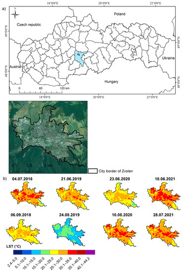
Figure 1.
(a) Location of the study area; (b) Calculated LST values for evaluated days between the years of 2018–2021.
2.2. Data Sources
A land cover map (focusing on vegetation in the settlement) was derived from databases provided by the Office of Geodesy, Cartography and Cadastre of the Slovak Republic [51], and was verified by field mapping. Land surface temperature calculation was based on Landsat−8 images from a satellite program operated by NASA and the U.S. Geological Survey [52]. All spatial data were reconciled to the EPSG:3035 (ETRS89, LAEA) Coordinate Reference System and all spatial analyses were conducted in ArcGIS version 10.3 (ESRI®). Statistical analyses were performed in R [53].
2.2.1. Data to Identify Vegetation in the City
To identify the land cover in the city, we used a combination of several data from the database provided by the Office of Geodesy, Cartography and Cadastre of the Slovak Republic [51], such as the Classified Point Cloud from the Airborne Laser Scanning (LAS version 1.4) [54] with a point cloud height accuracy of 0.05 m and a point cloud position accuracy of 0.07 m, the Orthophotomosaic of Slovakia with 4 channels (RGBN, 8-bit) and with an accuracy of 0.2 m per pixel [55], and the Basic Database for the Geographical Information System [49], which consists of data and metadata on spatial landscape features, their spatial and thematic attributes and their interrelationships.
2.2.2. Data for Land Surface Temperature Retrieval
Landsat satellites are widely used in monitoring and detecting environmental changes, especially for the retrieval of LST and NDVI (Normalized Difference Vegetation Index). Their extensive use has incentivized the development of well-documented techniques for optimal use [56,57]. The data were acquired from the U.S. Geological Survey website [52]. Eight images between 2018 and 2022 (Table 1) were used to determine the land surface temperature, of which the cooling effect of green spaces was subsequently determined. We selected eight days during the summer period on which cloudless satellite images were available and which corresponded to a year of airborne laser scanning.

Table 1.
Acquisition dates and parameters of the Landsat images used for this study.
Landsat satellite imageries were selected for the summer months from the start of June to the first week of September so that they were as cloud-free as possible (clouds less than 10%). The resolution of most Landsat bands is 30 m (panchromatic is 15 m), but it is different for thermal bands. The original resolution of the collected Thermal InfraRed band of Landsat-8 is 100 m, which has been in resampled up to 30 m [58]. Obtaining the surface reflectance and calculating the surface temperature required radiometric calibration and correction for atmospheric effects (detailed in Section 2.4 and Supplement A).
2.3. Identification of Vegetation and Land Cover in the City
To quantify the cooling effect depending on the vegetation structure (with trees or without trees) and the size of green spaces, we classified the area of the city into three basic surface types—green spaces covered with trees, green spaces without trees (grass, occasionally shrub) and no green spaces. We used the Classified Point Cloud from Airborne Laser Scanning [54] to identify trees, shrubs and buildings (Figure 2). We extracted the tree layer from the Classified Point Cloud by extracting points (used Point Filters in ArcGIS) classified as “High Vegetation” and created a 1 m resolution raster using the “LAS Point Stats As Raster” function (method POINT COUNT) in ArcGIS. Using the same procedure, we extracted the Medium Vegetation, Low Vegetation and Building point categories from the point cloud. Since the Airborne Laser Scanning of the area took place in the winter and spring months of 2019 [54], we used the Orthophotomosaic of Slovakia with 3 channels (RGB) from 2018 and the Orthophotomosaic of Slovakia with 4 channels (RGBN, 8-bit) from 2021 [55], in order to refine the identification of all the categories, but especially Low Vegetation (grass). From the orthophotomosaic with 4 channels, we also created an NDVI raster with a resolution of 1 m, which we used (together with visual identification from the orthophotomosaic and other data) to distinguish areas covered with vegetation from areas without vegetation. In addition to the aforementioned data, the ZBGIS® layer (geographic scale 1:5000), which is a spatial object-oriented database of the national infrastructure of spatial information on topographic objects in the Slovak Republic, was also included in the creation of the resulting land cover layer. By integrating the above data, and verifying and checking them each other, we created a landscape cover layer in which we distinguished the following categories: green spaces with high vegetation (trees), green spaces with medium vegetation (shrub), green spaces with low vegetation (grass), arable land, built-up areas (without vegetation), bare soil and water areas. Since the area of green spaces with medium vegetation and bare areas was low, we merged green spaces with low vegetation and with medium vegetation into one category (green grass spaces), and we merged the bare soils category with the building areas category into the urban area (urban matrix—buildings, roads, sidewalks). The two categories (trees and grass) of green spaces were further divided on the basis of size into three types: small (up to 1000 m2), medium (1000–10,000 m2) and large (over 10,000 m2). The small area threshold was based on the pixel size of the Landsat image (30 × 30 m) used to calculate the LST (Section 2.2.2 and Section 2.4). We also divided urban areas without vegetation into two categories based on size: small (up to 10,000 m2) and large (over 10,000 m2). Similar categories of urban land cover were also distinguished, for example, by [47]. We present the resulting categories in Table 2.
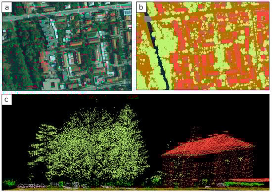
Figure 2.
Identification of vegetation and buildings; (a) Orthophotomosaic (a part of the city); (b) Classified Point Cloud obtained by Airborne Laser Scanning—LiDAR (a part of the city); (c) 3D visualization of LiDAR using ArcGIS 10.3 Legend for (b,c): red—buildings, light green—trees, green—shrub, brown—ground.
Table 2.
Categories of city land cover.
2.4. Land Surface Temperature Retrieval
A single-channel method was used to retrieve the land surface temperature. The thermal band 10 of the Landsat-8 OLI/TIRS was applied to determine the land surface temperature following [52,59,60]. The land surface temperature was calculated for eight days listed in Table 1. The steps of the procedure are given in Supplement A.
2.5. Statistical Analysis of Green Spaces Cooling Effect and Distance of Cooling Effect Analyses
To quantify differences in the magnitude of the cooling effect of green spaces and the distance from the edge of the green space over which the cooling effect occurs, we used several statistical methods presented below. We generated 3000 random points (with a minimum distance of 30 m from each other) within the city of Zvolen using the ArcGIS tool “Create Random Points”. Water bodies and arable land areas were excluded from generating random points. Using the ArcGIS tool “Extract Multi Values to Points”, the LST values calculated from LANDSAT images were extracted to random points. The values of distances from the boundaries of individual types of green space, distances from no vegetation areas and distances from water bodies were also extracted for each point. All distances were calculated with the ArcGIS “Euclidean Distance” tool.
2.5.1. Evaluation of Green Spaces Cooling Intensity
Differences in the LST among the different green space and their surroundings (category of no vegetation area) were tested with a one-way analysis of variance (ANOVA), followed by post hoc comparisons using the Tukey HSD method; this was performed after the homogeneity of variance was checked visually using a diagnostics graph [61]. In general, ANOVA tests the null hypothesis of the equality of the means (that there are no differences between the means of the values) between several independent groups by comparing the variability between them. If the variability between groups is improbably large (we test with an F-test), then we reject the null hypothesis of the equality of the means and consider the groups to be different [62,63,64].
2.5.2. Evaluation of the Green Spaces Cooling Distance
By verifying the consistency of the distribution of individual variable values with the normal probability distribution graphical comparison of the distribution using histograms and Q-Q graphs, we found that the distribution of the values of the distances from the boundaries of the individual green space categories do not correspond to the normal distribution. For this reason, the data were log-transformed to improve their normality. Our main objective was to confirm or refute the existence of a relationship between LST values of no vegetation areas and their distance from green spaces, and then to see if this dependence is different for green spaces of different vegetation structure (with trees or without trees) and size. The goal was not to find a model that would predict the values of the explained variable as accurately as possible. Since a preliminary evaluation of the correlation between the LST and distances (logarithmic values) from individual types of green space showed that the data could be expressed using a straight line, we used linear regression, because of the ease of interpreting the regression results and the parameters of the regression equation. We used the values of the Adjusted Coefficient of Determination (Radj2), intercept (β0) and slope of the line (β1) of the simple linear regression between LST and distance from individual types of green space in order to compare the significance of the cooling effect of different types of green space.
To more accurately identify the cooling distance, we classified the distance values of sample points from the boundaries of each green space category into 30 m wide distance intervals (0.1–30.0 m, 30.1–60.0 m, 60.1–90.0 m, etc.). As the maximum distances from the different green space categories varied (Table 3), it was possible to allocate different numbers of zones to the different green space categories. Therefore, the last zone “Z” starts at a different distance in each category and has a different width; it was set so that the last zone would also not contain less than 100 points. Since water bodies also have a cooling effect on their surroundings, we also classified the sample points in the same way into categories of distance from the boundaries of water bodies (the Hron River, the hydroelectric plants channel, the Môťová Dam, small bodies of water). Using a one-way analysis of variance, we then assessed the differences in the LST between varying zones of distance from each type of green space and water, and thus identified the distance at which LST values still showed a significant reduction.
Table 3.
Results of simple linear regression models between LST on each day assessed and the distance from the boundary of green spaces of different categories.
3. Results and Discussion
The distribution comparison of the LST calculated from Landsat images for the evaluated days is presented in Figure 3. These were mostly warm to very warm days, with the highest temperatures exceeding 30 °C and extremes (impervious surfaces) reaching 40 °C. This is except for 24 August 2019, which was a significantly cooler day compared to the others, when the highest calculated values exceeded only 20 °C.
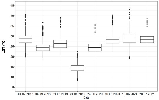
Figure 3.
Distribution comparison of land surface temperature (LST) calculated from Landsat images for the evaluated days in 2018–2021. Boxes indicate median and quartiles, and whiskers extend to the most extreme data points, not considering outliers (defined by 1.5 interquartile ranges). Data points outside the whiskers are outliers.
3.1. Cooling Intensity
Based on the results of the one-way analysis of variance, it can be concluded that a statistically significant difference was confirmed between Ul (large urban area without vegetation) and all the evaluated categories of green space. It can also be concluded that this difference, cooling intensity, is significantly different depending on the structure (with trees versus treeless) and the size of the green spaces. Comparisons of the median, minimum, and maximum LST values between the city land cover categories for the individual evaluated days during the years 2018–2021 are in the figures in Supplement B1 (years 2018–2019) and in Supplement B2 (years 2020–2021). A table in Supplement C presents the significance level of the multiple comparisons of the differences between the pairs of categories in the city land cover. These results confirm the findings of other authors. For example, [47] found a significant difference in the cooling effect between green areas covered with trees and those without trees (covered only with grass or shrubs). In addition, [46] reported that green spaces with a more complex vegetation structure (herbaceous layers, shrubs and trees) and without a management (irrigation, fertilization or pruning) had a higher capacity to provide air purification and climate regulation ESs. Similarly, [45] pointed to the dependence of the cooling effect on tree canopy cover and also on tree species. [65] using Landsat data and evaluating 39 parks in Shanghai, China, which vary from 0.96 to 140.22 ha. The results show that the parks’ LST decreased logarithmically with park size. Furthermore, [21] evaluated 92 parks ranging in size from 0.1 ha to 41.9 ha. They reported that a non-linear relationship existed between the park size and its cooling intensity, which in turn was mainly affected by the park’s composition of trees and shrubs. They mentioned that the cooling effect is more significant in large parks, especially in spring and summer.
The results further show that, in general, the warmer the day, the higher the cooling intensity of green spaces. During colder days (e.g., 24 August 2019), the cooling effect is less pronounced. This finding is in agreement with the findings of, e.g., [66,67]. Significantly, the largest cooling intensity effect is for GTl (large green spaces over 1 ha covered with trees), which are cooler than Ul by almost 4.5 °C on average and by almost 6 °C on the hottest days. In contrast, on a significantly cooler day (24 August 2019) compared to the other days assessed, GTls were cooler on average by just under 2.5 °C. (Figure 4). In addition, [68] measured the difference between the air temperature (mobile traverse method) of Beijing’s Olympic Forest Park in China and its surroundings. They also compared the difference between the LST (obtained from Landsat) of the park and its surroundings. They found that the air temperature during the day was in the range of 1.0–3.5 °C lower in the park than in the surrounding area, and that the surface temperature was in the range of 1.7–4.8 °C lower. Similarly, [45] observed the cooling intensity (by ground air temperature measurement) of 21 parks ranging from 0.85 to 22.3 ha in Addis Ababa, Ethiopia, with a mean value of 3.93 °C (ranging from 0.11 up to 6.72 °C). In addition, [22] found a difference between the temperature of the park in Wroclaw, Poland, and its surroundings that was in the range of 1.9 to 3.6 °C. This difference depended on the park size and land use type in the park’s surrounding area.
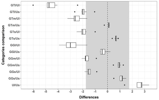
Figure 4.
Comparison of average LST differences between pairs of analyzed categories of town land cover for the entire evaluated period. Part I.: differences between urban categories (without vegetation) and categories of green space. Us—Urban small areas without vegetation, Ul—Urban large areas without vegetation, GGs—Green Grass small spaces, GGm—Green Grass medium spaces, GGl—Green Grass large spaces, GTs—Green Tree small spaces, GTm—Green Tree medium spaces, and GTl—Green Tree large spaces.
A smaller cooling effect was produced by the GGls (large green spaces over 1 ha without trees), whose LST was, on average, 2.9 °C lower than their Ul surroundings (Figure 4). On the hottest days, the cooling effect reached 4 °C, while on the coldest day it averaged around 1.6 °C. Looking at Figure 5, we can also see that the cooling intensity effect of GGls is, on average, 1.6 °C lower than that of GTls. The lower cooling intensity of the green spaces covered with low vegetation (grass or shrubs) compared to green spaces with high vegetation (trees) was also confirmed by the research of [69]. Almost similar to the effect of GGls are GTm (medium green spaces of 1000–10,000 m2 with trees), which are cooler compared to their Ul surroundings by 2.5 °C on average. In addition, when comparing them with each other (Figure 5), we see that the LST difference between them is about 0.54 °C on average. This difference increases to just over 0.7 °C on the hottest days, and on the coldest day (24 August 2019), there was no difference. That their cooling effect is usually almost the same is confirmed by the data in Supplement C, where we can see that there was a statistically significant difference between them on only three of the days evaluated (21 June 2019, 23 June 2020 and 10 August 2020). In addition, [47] showed that even green spaces with reduced areas (in his case 2.04 ha and 0.49 ha) can regulate the microclimate, alleviating the temperature by 1–3 °C.
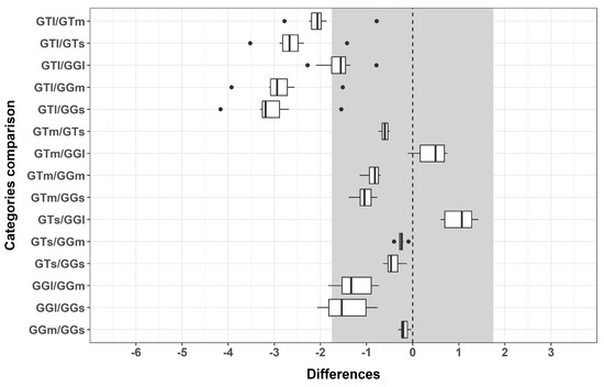
Figure 5.
Comparison of average LST differences between pairs of analyzed categories of town land cover for the entire evaluated period. Part II.: differences between categories of green spaces from each other. GGs—Green Grass small spaces, GGm—Green Grass medium spaces, GGl—Green Grass large spaces, GTs—Green Tree small spaces, GTm—Green Tree medium spaces, GTl—Green Tree large spaces.
The other categories of green space provide a cooling intensity effect below 2 °C (Figure 4). A slightly higher cooling effect (on average 1.9 °C) is provided by GTs (small green spaces up to 1000 m2 with trees) compared to GGm (medium green areas 1000–10,000 m2 without trees), being on average 1.7 °C, and GGs (small green areas up to 1000 m2 without trees), being on average 1.5 °C. Similar values were found, for example, by [70], who reported an average cooling intensity of 1 °C for green spaces between 300 m2 and 2300 m2 and a cooling intensity of 2 °C for slightly larger parks with an area between 650–5000 m2. The LST differences between the three categories (GTs, GGm and GGs) are on average below 0.5 °C (Figure 5), and a statistically significant difference was found in only one case (Supplement C), namely between GTs and GGs on 23 June 2020; therefore, the cooling effect of GTs, GGm and GGs can be considered more or less the same. In this context, the accuracy of LST determination from Landsat imagery using a single-channel algorithm should also be considered. Based on several works [69,71,72,73,74,75], we can assume that the degree of accuracy of our calculations (which will need to be verified by measurements in the future) is approximately 1.7 °C [48]. Hence, we can only assess the cooling effect with values up to 1.7 °C with some caution. Therefore, in Figure 4 and Figure 5, we have marked the differences between the LST values of each category that are smaller than 1.7 with a grey area. It is the difference between the surface temperature values of GGm and GGs and the surface temperature values of Ul (their cooling intensity) that reaches a value close to or slightly lower (GGs) than 1.7 °C, on average, over the period evaluated (Figure 4). The results show that the cooling intensity of GGm becomes more pronounced with the higher temperature reached during the day.
The results also show that Us (small urban areas up to 1 ha without vegetation) areas are statistically significantly cooler (Table in Supplement C) compared to Ul (large urban areas over 1 ha without vegetation) by an average of 2.6 °C (Figure 4). It can be assumed that the Us were cooled by the vegetation by which they are surrounded. Moreover, Us are even cooler than most categories of green spaces. Only GTl are, on average, 1.9 °C cooler and GGl are, on average, only 0.3 °C cooler than Us (Figure 4). GGl were statistically significantly cooler (Supplement C) on only two occasions (21 June 2019 and 23 June 2020). GTm have almost identical LST values as Us with no statistically significant differences (Figure 4, Supplement C). GTs are on average 0.7 °C warmer than Us (Figure 4, Supplement B and Supplement C). Similarly, GGm and GGs are warmer compared to Us by 0.9 °C and 1.1 °C on average, respectively.
3.2. Cooling Distance
3.2.1. Cooling Distance Evaluated by a Simple Regression Analysis
The results show that the LST varies statistically significantly with the distance from the boundaries of most green space categories (Table 3), and that this cooling distance varies with the character (with trees or without trees) and size of the green space. Table 3 shows the results of a simple regression analysis between the LST on each day assessed and the distance from the boundary of the green spaces of different categories. In Table 3, in the slope column, we report both the original value of the coefficient β1 (slope of regression line) of linear regression (which expresses the expected change in LST when the distance value increases by one unit) and its recalculated value. Since the distance data were log-transformed to improve their normality, we recalculated the β1 coefficients of all equations to a common comparison base for the change in LST when the distance changes by 1 m (Table 3). Based on these recalculated values, we can compare the cooling distance of each green space category with each other. The maximum distances from the boundaries of each green space category differ, due to the different density (small areas are denser) and distribution of each green space category. The differences in the cooling distance between the green space categories are also visible when comparing the progression of the LST change curves as the distance from the boundary of each green space category increases. Figures in Supplement D1 and D2 show the regression curves for each green space category for each day evaluated. As can be seen, the progression (shape) of the curves on different days is almost identical, differing only in the LST values achieved as a function of the temperature conditions of the particular day. For a better comparison of the cooling distance, we plotted the course of the regression curves for different categories of green spaces in a common graph. As mentioned above, the progression of the curves on each day is almost identical, so for the sake of clarity, Figure 6 shows the progression only for the day 28 July 2021, and comparisons of the progression of the regression dependencies for all days evaluated are shown in Supplement E1 (years 2018–2019) and in Supplement E2 (years 2020–2021).
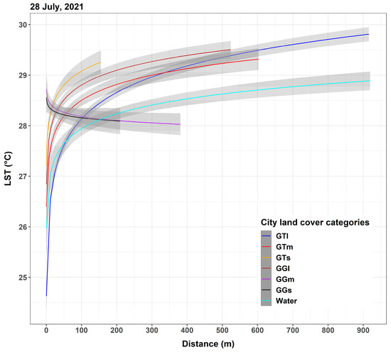
Figure 6.
Regression curves with a 99% confidence band of the dependence of LST on the distance from the borders of individual categories of green area and water on 28 July 2021.
Comparing the results in Table 3 and the course of the curves in Figure 6 (and Supplement E1 and E2), it can be concluded that, significantly, the largest impact, which also extends to the greatest distance, is for GTl (large green spaces over 1 ha with trees). By comparing the coefficient of determination (Radj2) values, we can conclude that GTl edge distance values typically explain about 30% (27.7–31.7%) of the variability in LST in the area, which is significantly more than explained by the edge distances of other green space categories. Only on the significantly coldest day (24 August 2019) was this only 17.3% (Table 3). In general, a trend can be observed that the warmer the day, the more the distribution of LST is influenced by the proximity of green areas and vice versa. Further, the edge of GTl has, on average, the lowest LST (highest cooling effect) compared to the LST values at the edge of the other green space categories, as can be seen from the Intercept values in Table 3. The Intercept values (coefficient β0 of the regression equation) represent the average LST at zero distance from the edge of the green space (right at its edge). The magnitude of the cooling distance is also indicated by the shape of the regression curves (Figure 6, Supplement E). From their waveforms, it can be seen that the LST increases most slowly with the distance from GTl, and hence that the cooling distance is greatest.
Based on the results in Table 3, Figure 6 and Supplement E, the ranking of the other categories of green space in terms of cooling distance is as follows. Medium green spaces with trees (GTm) have the second most significant effect on reducing ambient temperature, followed closely by large green spaces without trees (GGl). Although distance from the edge of GTm explains only 4.6–7.5% of the variability in the distribution of the LST in the area, compared to 7.0–19.3% for GGl (Radj2 in Table 3), we see that GTm reduce the LST in their surroundings more and to a greater distance when comparing the progression of the regression curves (Figure 6, Supplement E). The above conclusion is supported by the results in Table 3, from which we see that the LST values at the GTm boundary are similar to those at the GGl boundary (values in the intrc column); however, the recalculated (back-transformed) slope of the regression line (Table 3) is usually slightly lower for GTm, implying a slower increase in LST with distance from their boundary.
Even to a lesser distance, but still demonstrable, is the cooling effect of GTs, which explain, on average, only about 4% (1.3–5.6%) of the variability in the LST distribution in the area. The average values of LST at their boundary are slightly higher compared to the previous categories, and the recalculated values of the slope of the regression line are, in turn, higher, as confirmed by the regression curve in Figure 6.
No effect on the cooling of their surroundings was shown by our results for medium and small green spaces without trees (GGm and GGs), which, on average, do not explain even a percentage of the variability in the LST; they have the significantly highest values of LST at their boundary, negative values in the slope of regression line and in three cases, the relationship between the distribution of LST and the distance from their boundary was not even significant (Table 3, Figure 6, Supplement E).
For comparison, we also assessed the cooling distance from water bodies. From the results, it can be concluded that the cooling distance of water areas is slightly lower compared to GTl (Figure 6), but higher than the cooling distance of the other categories of green space. The average LST values are significantly higher at the boundary of water areas compared to the average LST at the boundary of GTl (column intrc in Table 3). Up to a distance of approximately 100 m, the cooling effect is higher at GTl. At distances greater than 100 m, the regression model curve shape differs significantly from the other curves—asymptotically reaching significantly lower maximum LST values at greater distances from the water body boundary than the curves at the other green space boundaries (Figure 6). However, this low LST value of the distant surroundings of the water spaces is due to the inclusion in its calculation of the LST values within GTl (which are low); this, in turn, is logically not included in the calculation of the LST values of the distant surroundings of GTl. Thus, it is not a consequence of the cooling effect of water bodies, which extends from water bodies to approximately 90 m from their boundaries (detailed in Section 3.2.1).
3.2.2. Cooling Distance Evaluated by One-Way Analysis of Variance
To more accurately identify the cooling distance, we classified the distance values of sample points from the boundaries of each green space category into 30 m wide distance intervals. Supplement F1 and Supplement F2 show boxplots of the distribution of LST values (median, quartiles, outliers) versus 30 m zones for each green space category from 28 July 2021. On other days, the temperature distributions within the 30 m zones look almost identical (as confirmed by the shape of the curves in Supplement D and E). The conclusions stated in the previous chapter are evident from the graphs, namely, that the greatest cooling effect and to the greatest distance is manifested at GTl. For GGm and GGs, the cooling distance has not been demonstrated. For GTm and GGl, the effect is similar, but the temperature reduction extends to a greater distance for GTm. In contrast, the cooling intensity (temperature difference with respect to the distant surroundings) of the first 30 m zone is greater for GGl. Some of the above facts become more apparent when the average LST differences between the distance zones are displayed. Figure 7 shows comparisons of all the three categories of green area with trees (GTl, GTm, GTs) and Figure 8 shows comparisons of the GGl and water categories. In the plots, the value of 1.7 °C (dashed line) shows the value of the difference in LST between distance zones, which should be considered with some caution due to the accuracy of LST determination from satellite imagery (more in Section 3.1).
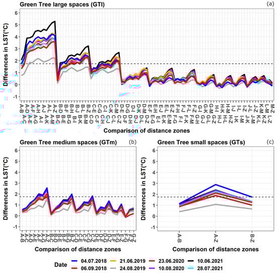
Figure 7.
Average LST differences between zones of distances from the boundaries of each category for all days assessed; (a) Green Trees large spaces; (b) Green Trees medium spaces; (c) Green Trees small spaces. A = 0–30 m, B = 30–60 m, C = 60–90 m, D = 90–120 m, E = 120–150 m, F = 150–180 m, G = 180–210 m, H = 210–240 m, I = 240–270 m, J = 270–300 m, K = 300–330 m, L = 330–360 m, M = 360–390 m, Z = over the previous distance—alternatively.
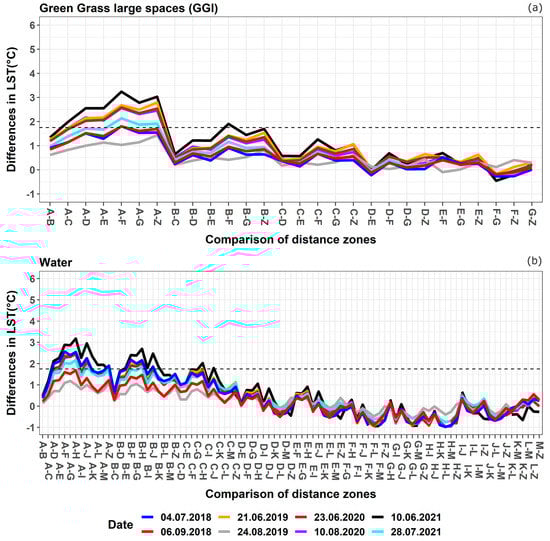
Figure 8.
Average LST differences between zones of distances from (a) Green Grass large spaces (GGl) boundaries; (b) Water. A = 0–30 m, B = 30–60 m, C = 60–90 m, D = 90–120 m, E = 120–150 m, F = 150–180 m, G = 180–210 m, H = 210–240 m, I = 240–270 m, J = 270–300 m, K = 300–330 m, L = 330–360 m, M = 360–390 m, Z = over the previous distance—alternatively.
Since, according to the results obtained, GGm and GGs have no cooling effect on their surroundings, we have shown plots of the average LST differences between the distance zones of these categories only in Supplement G. Table Supplement H summarizes the results of the analysis of variance of the statistical significance of the differences between each of the LST values between the distance zones from the boundaries of each green space category for all the days evaluated. As the outputs of the statistical analysis are extensive, we provide only a simplified summary of them in Supplement H. If the LST of a particular distance zone was significantly different from the LST of all or almost all the other distance zones (often between adjacent zones, e.g., A–B or B–C, there may not yet be a difference), the label all is included in Supplement H. If the LST values of a zone were not different from all, but only from the most distant zones (e.g., if the LST in zone D was statistically significantly different only from the LSTs in zones L, M, Z), only the number of zones that were different is noted in Supplement H (in the example above, this would be 3).
From the graphs (Figure 7 and Figure 8) and the data in Supplement H, we can see that for GTl, the significant cooling distance extends out to 90 m (zones A–C), and that the difference between LSTs near GTl (within 30 m, zone A) and areas more than 390 m away (zone Z) can exceed over 5 °C on the hottest days. However, some influence, which is less significant, extends out to 180 m (zone F), with a larger distance on warmer days and a smaller distance on cooler days (24 August 2019).
At GTm, the cooling effect is lower. The difference between LSTs in their vicinity (within 30 m, zone A) and areas more than 240 m away (zone Z) can exceed 2.5 °C on the warmest days (Figure 7).The cooling distance is similar to GTl, but with a lower cooling effect. A significant effect extends to 90 m (zone C) and a smaller effect extends to 150 m (zone E).
The study of [22], conducted in in Wroclaw (Poland), found a park cooling effect from approximately 130–170 to a maximum of 895–925 m, with LST differences from 0.7–3.2 °C to up to 15 °C, depending on the park size and the direction of orientation (north, west, etc.). Further, [76] found that, in a study on Tama New Town’s Central Park in Japan, a park of about 60 ha can reduce the air temperature at midday in a busy commercial area 1 km downwind by up to 1.5 °C. They further reported that, when there is no predominant wind, the cooling effects of the park extend almost equally in all directions and the area of influence extends only about 100 m from the park. Similarly, [65] found that, in Shanghai, China, the maximum cooling distance showed large variations from 64 m to 1405 m in relation to the park area (39 parks, from 0.96 to 140.22 ha), and that the cooling distance of most parks was limited to 600 m.
The cooling effect of GGl in their close proximity (within 30 m, Zone A) is slightly higher than for GTm, where the difference between LSTs in their vicinity (within 30 m) and areas are more distant (above 150 m) and can exceed over 3 °C on the hottest days (Figure 8). However, the cooling effect extends to a shorter distance than for GTm (Supplement H). A more pronounced effect extends to 30–60 m (zones A, B) and a less pronounced effect extends to 90 m (zone C); on the hottest days, this is up to 120 m (zone D).
The cooling distance of GTs was difficult to assess as it was only possible to create three distance zones (0–30, 30–60 and over 60 m, Supplement H). The results show that the demonstrable impact extends at least to 60 m. The difference between the LSTs close to them (within 30 m) and further away (over 60 m, zone Z) can exceed over 2.5 °C on the hottest days (Figure 7).
The results did not show a cooling effect for GGm and GGs; rather, the results show the opposite trend, in which areas close to them (within 30 m) are often warmer on average than those further away (Supplement G). This is due to the fact that the furthest points from these surfaces often lie on the GTl surface, which has a low LST value.
Our results are in agreement with the measurements of [47], who found that green spaces with trees had higher a cooling intensity and cooling distance compared to green spaces without trees (which showed mostly non-significant correlations in relation to the cooling effect). For green spaces with trees of 0.5–2 ha, they report a cooling distance of 60 m and up to 120 m in summer. Similarly, [23] found a cooling distance of 60–80 m for small surfaces with trees (area up to 1.2 ha). The authors of [45] studied the surface and air temperature in 21 parks (ranging from 0.85 to 22.3 ha) in Addis Ababa and found a maximum cooling intensity of 6.72 °C and a maximum estimated cooling distance of 240 m.
To compare the significance, we also assessed the cooling distance of water bodies. In addition, the results of the analysis of variance confirm the regression analysis outputs and show that the cooling distance of water bodies is lower than for GTl, but similar to or slightly higher than for GTm. The difference between LSTs in their vicinity (within 30 m, Zone A) and more distant areas (above 210 m) can exceed 3 °C on the hottest days (Figure 8). The cooling distance extends to approximately 90 m (zone C), although based on the results of the ANOVA analysis (Supplement H), the distance of the cooling effect is shorter than for GTm; the results are influenced by the fact that water bodies are not evenly distributed in the area and many of the sample points are at greater distances from them, often located in large green surfaces with trees (low LSTs). This fact has caused the average LST of the outermost zones (against which the LSTs of nearby zones are compared) to be lower than for other categories (Figure 6, Supplement E). In addition, for water bodies, it should be noted that we did not distinguish this category by size, which would most likely lead to large water bodies having a more pronounced cooling effect (cooling intensity and cooling distance) than GTl.
4. Conclusions
Based on the results obtained, it can be concluded that the cooling intensity, as well as cooling distance, are dependent on the size and structure (grass versus trees) of the green space. At the same time, the vegetation structure of the green space has a slightly greater influence on the cooling effect compared to the size of the green space, as indicated by the fact that medium (0.1–1 ha) green spaces with trees (GTm) have a similar, only slightly lower cooling intensity and, conversely, a greater cooling distance compared to large (over 1 ha) grass green spaces (GGl). Medium (0.1–1 ha) and small (up to 0.1 ha) grass green spaces (GGm and GGs) have a statistically significant cooling intensity, but their cooling effect towards the surroundings (cooling distance) has not been demonstrated. In contrast, small (up to 0.1 ha) green spaces with trees (GTs) have a slightly higher cooling intensity compared to GGm and GGs; their cooling effects on their surroundings is also statistically significant.
The most significant cooling effect is provided by large (over 1 ha) green spaces with trees (GTl), where the cooling intensity (difference of LST compared to an urban area without vegetation) was almost 4.5 °C on average (maximum almost 6 °C) and the cooling distance was significant up to 90 m (less significant up to 180 m). As mentioned above, GGl and GTm have similar effects, with a higher cooling intensity (2.9 °C versus 2.5 °C on average) for GGl; however, the cooling effect (cooling distance) extends to a greater distance (up to 90 m) for GTm compared to GGl, where the cooling effect only extends to 30–60 m. Small areas with trees (GTs) and medium and small areas without trees (GGm and GGs) have an average cooling intensity below 2 °C; for GGm and GGl, this is even below 1.7 °C. This is the threshold below which the differences should already be evaluated with some caution due to the accuracy of LST determination using the Single-Channel Algorithm from Landsat imagery [48]. For GTs, their cooling effect on their surroundings was significant and extends to at least 60 m. For GGm and GGs, their cooling effect their surroundings was not demonstrated.
Several authors proposed different threshold values for the size of green spaces in relation to the cooling effect, depending on different latitudes, altitudes, climatic conditions, temperature extremes (warm, extremely warm), and urban contexts, but also proposed different selection samples in the study (minimum size of green area) and definition of the cooling effect, as an example [77]. The values they found range from 0.4 to 20 ha. According to our results, areas as small as about 0.1 ha show a demonstrable cooling effect if they are covered with trees. For grass spaces without trees, a size of over 1 ha is needed in order to achieve a cooling effect on the surrounding area. However, we are aware that the obtained results have some limitations related to the LST determination method (accuracy mentioned above), the minimum assessment area (Landsat pixel size 8–100 m pixel resampled to 30 m) and the well-known problem of mixed pixels in remote sensing [21]. Moreover, the LST values were only calculated at one time (around 10:30 am) during the day, not assessing the co-occurrence of shading by buildings. Therefore, the future refinement of measurements for the in situ air temperature will need to be made at more times of the day, as well as at night.
The findings are applicable to urban management because they quantify the parameters of green spaces (vegetation composition and area size), the magnitude of the cooling effect and the distance to which the cooling occurs in an exact way. This knowledge can be directly used to plan sustainable urban design in terms of mitigating extreme heat, as well as to implement remedial measures in existing urban systems. They allow planners to effectively respond to the increased need for the cooling of urban space, particularly, for example, in local hotspots within an urban heat island, which, at exposed times, have high concentrations of heat-exposed residents or vulnerable populations such as children or elderly people. Such natural mitigation solutions are also important elements of urban green infrastructure, which provides multiple ecosystem services and has a strong self-regulatory capacity.
Supplementary Materials
The following supporting information can be downloaded at: https://www.mdpi.com/article/10.3390/su15043705/s1, Supplements A–H. References [78,79,80,81,82] are cited in the supplementary materials.
Author Contributions
Conceptualization, I.G. and B.O.; methodology, I.G., B.O., V.M. and Z.G.; software, I.G. and V.M. validation, I.G. and B.O.; formal analysis, I.G.; resources, B.O..; data curation, V.M. and I.G.; writing—original draft preparation, I.G. and Z.G.; writing—review and editing, I.G. and B.O.; visualization, I.G. and V.M.; supervision, B.O.; funding acquisition, B.O. All authors have read and agreed to the published version of the manuscript.
Funding
This research was funded by project Comprehensive research of determinants for ensuring environmental health (ENVIHEALTH), grant no. ITMS 313011T721 supported by the Operational Programme Integrated Infrastructure (OPII) funded by the ERDF.
Data Availability Statement
Not applicable.
Conflicts of Interest
The authors declare no conflict of interest. The funders had no role in the design of the study; in the collection, analyses, or interpretation of data; in the writing of the manuscript; or in the decision to publish the results.
References
- Pickett, S.T.A.; Cadenasso, M.L.; Grove, J.M.; Nilon, C.H.; Pouyat, R.V.; Zipperer, W.C. Urban ecological systems: Linking terrestrial ecological, physical, and socioeconomic components of metropolitan areas. In Urban Ecology. An International Perspective on the Interaction Between Humans and Nature; Marzluff, J., Shulenberger, E., Endlicher, W., Bradley, G., Simon, U., Alberti, M., Ryan, C., ZumBrunnen, C., Eds.; Springer: New York, NY, USA, 2008; pp. 99–122. [Google Scholar] [CrossRef]
- Oke, T.R.; Mills, R.; Christen, A.; Voogt, J.A. Urban Climates; Cambridge University Press: Cambridge, UK, 2017; p. 519. [Google Scholar] [CrossRef]
- Kuttler, W. The urban climate—Basic and applied aspects. In Urban Ecology. An International Perspective on the Interaction Between Humans and Nature; Marzluff, J., Shulenberger, E., Endlicher, W., Bradley, G., Simon, U., Alberti, M., Ryan, C., ZumBrunnen, C., Eds.; Springer: New York, NY, USA, 2008; pp. 233–248. [Google Scholar] [CrossRef]
- Gartland, L. Heat Islands. Understanding and Mitigating Heat in Urban Areas; Routledge: London, UK, 2008; p. 215. [Google Scholar] [CrossRef]
- Poumadere, M.; Mays, C.; Le Mer, S.; Blong, R. The 2003 heat wave in France: Dangerous climate change here and now. Risk Anal. 2005, 25, 1483–1494. [Google Scholar] [CrossRef]
- Hondula, D.M.; Davis, R.E.; Leisten, M.J.; Saha, M.V.; Veazey, L.M.; Wegner, C.R. 2012: Fine-scale spatial variability of heat-related mortality in Philadelphia county, USA, from 1983-2008: A case-series analysis. Environ. Health 2012, 11, 16. [Google Scholar] [CrossRef]
- Su, M.A.; Ngarambe, J.; Santamouris, M.; Yun, G.Y. Empirical evidence on the impact of urban overheating on building cooling and heating energy consumption. iScience 2021, 24, 102495. [Google Scholar] [CrossRef]
- White, M.A.; Nemani, R.R.; Thornton, P.E.; Running, S.W. Satellite evidence of phenological differences between urbanized and rural areas of the eastern United States deciduous broadleaf forest. Ecosystems 2002, 5, 260–277. [Google Scholar] [CrossRef]
- Irmak, M.A.; Yilmaz, S.; Dursun, D. Effect of different pavements on human thermal comfort conditions. Atmósfera 2017, 30, 355–366. [Google Scholar] [CrossRef]
- Garcia-Nevado, E. Termografía del Cañón Urbano: Uso de la Perspectiva para una Evaluación Térmica Global de la Calle. Ph.D. Thesis, Universitat Politecnica de Catalunya, Barcelona, Spain, 2019; p. 606. [Google Scholar]
- Yezioro, A.; Capeluto, I.G.; Shaviv, E. Design guidelines for appropriate insolation of urban squares. Renew. Energy 2006, 31, 1011–1023. [Google Scholar] [CrossRef]
- Ali-Toudert, F.; Mayer, H. Effects of asymmetry, galleries, overhanging facades and vegetation on thermal comfort in urban street canyons. Sol. Energy 2007, 81, 742–754. [Google Scholar] [CrossRef]
- Hong, C.; Yang, Y.; Ge, S.; Chai, G.; Zhao, P.; Shui, Q.; Gu, Z. Is the design guidance of color and material for urban buildings a good choice in terms of thermal performance? Sustain. Cities Soc. 2022, 83, 103927. [Google Scholar] [CrossRef]
- Susca, T.; Gaffin, S.R.; Dell’Osso, G.R. Positive effects of vegetation: Urban heat island and green roofs. Environ. Pollut. 2011, 159, 2119–2126. [Google Scholar] [CrossRef]
- Lobaccaro, G.; Acero, J.A. Comparative analysis of green actions to improve outdoor thermal comfort inside typical urban street canyons. Urban Clim. 2015, 14, 251–267. [Google Scholar] [CrossRef]
- Aram, F.; García, E.H.; Solgi, E.; Mansournia, S. Urban green space cooling effect in cities. Review article. Heliyon 2019, 5, e01339. [Google Scholar] [CrossRef]
- Zhang, Q.; Zhou, D.; Xu, D.; Rogora, A. Correlation between cooling effect of green space and surrounding urban spatial form: Evidence from 36 urban green spaces. Build. Environ. 2022, 222, 109375. [Google Scholar] [CrossRef]
- Oliveira, S.; Andrade, H.; Vaz, T. The cooling effect of green spaces as a contribution to themitigation of urban heat: A case study in Lisbon. Build. Environ. 2011, 46, 2186–2194. [Google Scholar] [CrossRef]
- Shashua-Bar, L.; Pearlmutter, D.; Erell, E. The cooling efficiency of urban landscape strategies in a hot dry climate. Landsc. Urban Plann. 2009, 92, 179–186. [Google Scholar] [CrossRef]
- Mackey, C.W.; Lee, X.; Smith, R.B. Remotely sensing the cooling effects of city scale efforts to reduce urban heat island. Build. Environ. 2012, 49, 348–358. [Google Scholar] [CrossRef]
- Cao, X.; Onishi, A.; Chen, J.; Imura, H. Quantifying the cool island intensity of urban parks using ASTER and IKONOS data. Landsc. Urban Plann. 2010, 96, 224–231. [Google Scholar] [CrossRef]
- Blachowski, J.; Hajnrych, M. Assessing the cooling effect of four urban parks of different sizes in a temperate continental climate zone: Wroclaw (Poland). Forests 2021, 12, 1136. [Google Scholar] [CrossRef]
- Shashua-Bar, L.; Hoffman, M.E. Vegetation as a climatic component in the design of an urban street. An empirical model for predicting the cooling effect of urban green areas with trees. Energy Build. 2000, 31, 221–235. [Google Scholar] [CrossRef]
- Teixeira, C.F.B. Green space configuration and its impact on human behavior and urban environments. Urban Clim. 2021, 35, 100746. [Google Scholar] [CrossRef]
- Sun, C.Y. A street thermal environment study in summer by the mobile transect technique. Theor. Appl. Climatol. 2011, 106, 433–442. [Google Scholar] [CrossRef]
- Yan, H.; Wu, F.; Dong, L. Influence of a large urban park on the local urban thermal environment. Sci. Total Environ. 2018, 622–623, 882–891. [Google Scholar] [CrossRef] [PubMed]
- Park, J.; Kim, J.H.; Sohn, W.; Lee, D.-K. Urban cooling factors: Do small greenspaces outperform building shade in mitigating urban heat island intensity? Urban For. Urban Green. 2021, 64, 127256. [Google Scholar] [CrossRef]
- Yan, L.; Jia, W.; Zhao, S. The cooling effect of urban green spaces in metacities: A case study of Beijing, China’s capital. Remote Sens. 2021, 13, 4601. [Google Scholar] [CrossRef]
- Nichol, J.E.; Fung, W.Y.; Lam, K.; Wong, M.S. Urban heat island diagnosis using ASTER satellite images and ‘in situ’ air temperature. Atmos. Res. 2009, 94, 276–284. [Google Scholar] [CrossRef]
- Arnfield, A.J. Two decades of urban climate research: A review of turbulence, exchanges of energy and water, and the urban heat island. Int. J. Climatol. 2003, 23, 1–26. [Google Scholar] [CrossRef]
- Zhou, W.; Huang, G.; Cadenasso, M.L. Does spatial configuration matter? Understanding the effects of land cover pattern on land surface temperature in urban landscapes. Landsc. Urban Plann. 2011, 102, 54–63. [Google Scholar] [CrossRef]
- Masoudi, M.; Tan, P.Y.; Liew, S.C. Multi-city comparison of the relationships between spatial pattern and cooling effect of urban green spaces in four major Asian cities. Ecol. Indic. 2019, 98, 200–213. [Google Scholar] [CrossRef]
- Weng, Q.; Lu, D. A sub-pixel analysis of urbanization effect on land surface temperature and its interplay with impervious surface and vegetation coverage in Indianapolis, United States. Int. J. Appl. Earth Obs. Geoinf. 2008, 10, 68–83. [Google Scholar] [CrossRef]
- Kim, S.W.; Brown, R.D. Urban heat island (UHI) variations within a city boundary: A systematic literature review. Renew. Sustain. Energy Rev. 2021, 148, 111256. [Google Scholar] [CrossRef]
- Grimmond, C.S.B.; Roth, M.; Oke, T.R.; Au, Y.C.; Best, M.; Betts, R.; Carmichael, G.; Cleugh, H.; Dabberdt, W.; Emmanuel, R.; et al. Climate and more sustainable cities: Climate information for improved planning and management of cities (Producers/capabilities perspective). Procedia Environ. Sci. 2010, 1, 247–274. [Google Scholar] [CrossRef]
- Armson, D.; Stringer, P.; Ennos, A.R. The effect of street trees and amenity grass on urban surface water runoff in Manchester, UK. Urban For. Urban Green. 2013, 12, 282–286. [Google Scholar] [CrossRef]
- Gómez-Baggethun, E.; Barton, D.N. Classifying and valuing ecosystem services for urban planning. Ecol. Econ. 2013, 86, 235–245. [Google Scholar] [CrossRef]
- Pinho, P.; Correia, O.; Lecoq, M.; Munzi, S.; Vasconcelos, S.; Gonçalves, P.; Rebelo, R.; Antunes, C.; Silva, P.; Freitas, C.; et al. Evaluating green infrastructure in urban environments using a multi-taxa and functional diversity approach. Environ. Res. 2016, 147, 601–610. [Google Scholar] [CrossRef] [PubMed]
- Villalobos-Jiménez, G.; Dunn, A.M.; Hassall, C. Dragonflies and damselflies (Odonata) in urban ecosystems: A review. Eur. J. Entomol. 2016, 113, 217–232. [Google Scholar] [CrossRef]
- Langemeyer, J. Urban Ecosystem Services. The Value of Green Spaces in Cities. Ph.D. Thesis, Stockholm Resilience Centre, Stockholm University, Stockholm, Sweden, 2015; p. 246. [Google Scholar]
- Mexia, T.; Vieira, J.; Príncipe, A.; Anjos, A.; Silva, P.; Lopes, N.; Freitas, C.; Santos-Reis, M.; Correia, O.; Branquinho, C.; et al. Ecosystem services: Urban parks under a magnifying glass. Environ. Res. 2018, 160, 469–478. [Google Scholar] [CrossRef] [PubMed]
- Constanza, R.; D’Arge, R.; De Groot, R.; Farber, S.; Grasso, M.; Hannon, B.; Limburg, K.; Naeem, S.; O’Neill, R.V.; Paruelo, J.; et al. The value of the world’s ecosystem services and natural capital. Nature 1997, 387, 253–260. [Google Scholar] [CrossRef]
- Derkzen, M.L.; van Teeffelen, A.J.A.; Verburg, P.H. Quantifying urban ecosystem services based on highresolution data of urban green space: An assessment for Rotterdam, the Netherlands. J. Appl. Ecol. 2015, 52, 1020–1032. [Google Scholar] [CrossRef]
- Xie, M.; Wang, Y.; Chang, Q.; Fu, M.; Ye, M. Assessment of landscape patterns affecting land surface temperature in different biophysical gradients in Shenzhen, China. Urban Ecosyst. 2013, 16, 871–886. [Google Scholar] [CrossRef]
- Feyisa, G.L.; Dons, K.; Meilby, H. Efficiency of parks in mitigating urban heat island effect: An example from Addis Ababa. Landsc. Urban Plann. 2014, 123, 87–95. [Google Scholar] [CrossRef]
- Vieira, J.; Matos, P.; Mexia, T.; Silva, P.; Lopes, N.; Freitas, C.; Correia, O.; Santos-Reis, M.; Branquinho, C.; Pinho, P. Green spaces are not all the same for the provision of air purification and climate regulation services: The case of urban parks. Environ. Res. 2018, 160, 306–313. [Google Scholar] [CrossRef]
- Grilo, F.; Pinho, P.; Aleixo, C.; Catita, C.; Silva, P.; Lopes, N.; Freitas, C.; Santos-Reis, M.; McPhearson, T.; Branquinho, C. Using green to cool the grey: Modelling the cooling effect of green spaces with a high spatial resolution. Sci. Total Environ. 2020, 724, 138182. [Google Scholar] [CrossRef]
- Murtinová, V.; Gallay, I.; Olah, B. Mitigating effect of urban green spaces on surface urban heat island during summer period on an example of a medium size town of Zvolen, Slovakia. Remote Sens. 2022, 14, 4492. [Google Scholar] [CrossRef]
- ZBGIS®. Basic Database for the Geographic Information System. Geodetic and Cartographic Institute Bratislava (GKÚ) Slovakia. Available online: https://zbgis.skgeodesy.sk/mkzbgis/sk/zakladna-mapa?pos=48.800000,19.530000,8 (accessed on 10 November 2022).
- Corine Land Cover 2018. Copernicus Land Monitoring Service. Available online: https://land.copernicus.eu (accessed on 5 April 2022).
- ÚGKK SR: Geodesy, Cartography and Cadastre Authority of the Slovak Republic. Geoportal. Available online: https://www.geoportal.sk/en/ (accessed on 9 August 2022).
- United States Geological Survey EarthExplorer. Available online: https://earthexplorer.usgs.gov/ (accessed on 10 November 2022).
- R Core Team. R: A Language and Environment for Statistical Computing. R Foundation for Statistical Computing, Vienna, Austria. Available online: https://www.R-project.org/ (accessed on 10 November 2022).
- Airborne Laser Scanning. ÚGKK SR: Geodesy, Cartography and Cadastre Authority of the Slovak Republic. Geoportal. Available online: https://www.geoportal.sk/en/zbgis/als_dmr/ (accessed on 9 August 2022).
- Orthophotomosaic of Slovakia. ÚGKK SR: Geodesy, Cartography and Cadastre Authority of the Slovak Republic. Geoportal. Available online: https://www.geoportal.sk/en/zbgis/orthophotomosaic/ (accessed on 9 August 2022).
- Derdouri, A.; Wang, R.; Murayama, Y.; Osaragi, T. Understanding the links between LULC changes and SUHI in cities: Insights from two-decadal studies (2001–2020). Remote Sens. 2021, 13, 3654. [Google Scholar] [CrossRef]
- Klok, L.; Zwart, S.; Verhagen, H.; Mauri, E. The surface heat island of Rotterdam and its relationship with urban surface characteristics. Resour. Conserv. Recycl. 2012, 64, 23–29. [Google Scholar] [CrossRef]
- Landsat Satellite Missions. United States Geological Survey. Available online: https://www.usgs.gov/landsat-missions/landsat-satellite-missions (accessed on 10 November 2022).
- Idi, B.Y.; Maiha, A.I.; Abdullahi, M. Spatial mapping and monitoring thermal anomaly and radiative heat flux using Landsat-8 thermal infrared data—A case study of Lamurde hot spring, upper part of Benue trough, Nigeria. J. Appl. Geophys. 2022, 203, 104654. [Google Scholar] [CrossRef]
- Ndossi, M.I.; Avdan, U. Application of open source coding technologies in the production of land surface temperature (LST) maps from Landsat: A PyQGIS plugin. Remote Sens. 2016, 8, 413. [Google Scholar] [CrossRef]
- Lepš, J.; Šmilauer, P. Biostatistics with R: An Introductory Guide for Field Biologists, 1st ed.; Cambridge University Press: Cambridge, UK, 2020; p. 382. [Google Scholar] [CrossRef]
- Zar, J.H. Biostatistical Analysis, 5th ed.; Prentice-Hall/Pearson: Upper Saddle River, NJ, USA, 2010; p. 944. [Google Scholar]
- Logan, M. Biostatistical Design and Analysis Using, R. A Practical Guide; Wiley-Blackwell: Hoboken, NJ, USA, 2010; p. 546. [Google Scholar] [CrossRef]
- Le, C.T.; Eberly, L.E. Introductory Biostatistics, 2nd ed.; Wiley: Hoboken, NJ, USA, 2016; p. 592. [Google Scholar]
- Cheng, X.; Wei, B.; Chen, G.; Li, J.; Song, C. Influence of park size and its surrounding urban landscape patterns on the park cooling effect. J. Urban Plann. Dev. 2015, 141, A4014002. [Google Scholar] [CrossRef]
- Cohen, P.; Potchter, O.; Matzarakis, A. Daily and seasonal climatic conditions of green urban open spaces in the Mediterranean climate and their impact on human comfort. Build. Environ. 2012, 51, 285–295. [Google Scholar] [CrossRef]
- Du, C.; Jia, W.; Chen, M.; Yan, L.; Kai, W. How can urban parks be planned to maximize cooling effect in hot extremes? Linking maximum and accumulative perspectives. J. Environ. Manag. 2022, 317, 115346. [Google Scholar] [CrossRef]
- Amani-Beni, M.; Zhang, B.; Xie, G.-D.; Odgaard, A.J. Impacts of the microclimate of a large urban park on its surrounding built environment in the summertime. Remote Sens. 2021, 13, 4703. [Google Scholar] [CrossRef]
- Adulkongkaew, T.; Satapanajaru, T.; Charoenhirunyingyos, S.; Singhirunnusorn, W. Effect of land cover composition and building configuration on land surface temperature in an urban-sprawl city, case study in Bangkok metropolitan area, Thailand. Heliyon 2020, 6, E04485. [Google Scholar] [CrossRef]
- Park, J.; Kim, J.-H.; Lee, D.K.; Park, C.Y.; Jeong, S.G. The influence of small green space type and structure at the streetlevel on urban heat island mitigation. Urban For. Urban Green. 2017, 21, 203–212. [Google Scholar] [CrossRef]
- Li, F.; Jackson, T.J.; Kustas, W.P.; Schmugge, T.J.; French, A.N.; Cosh, M.H.; Bindlish, R. Deriving land surface temperature from Landsat 5 and 7 during SMEX02/SMACEX. Remote Sens. Environ. 2004, 92, 521–534. [Google Scholar] [CrossRef]
- Yu, X.; Guo, X.; Wu, Z. Land surface temperature retrieval from landsat 8 TIRS—Comparison between radiative transfer equation-based method, split window algorithm and single channel method. Remote Sens. 2014, 6, 9829–9852. [Google Scholar] [CrossRef]
- García-Santos, V.; Cuxart, J.; Martínez-Villagrasa, D.; Jiménez, M.A.; Simó, G. Comparison of three methods for estimating land surface temperature from landsat 8-TIRS sensor data. Remote Sens. 2018, 10, 1450. [Google Scholar] [CrossRef]
- Laraby, K.G.; Schott, J.R. Uncertainty estimation method and Landsat 7 global validation for the Landsat surface temperature product. Remote Sens. Environ. 2018, 216, 472–481. [Google Scholar] [CrossRef]
- Jiang, Y.; Lin, W.A. Comparative analysis of retrieval algorithms of land surface temperature from landsat-8 data: A case study of Shanghai, China. Int. J. Environ. Res. Public Health 2021, 18, 5659. [Google Scholar] [CrossRef]
- Ca, V.T.; Asaeda, T.; Abu, E.M. Reduction in air conditioning energy caused by a nearby park. Energy Build. 1998, 29, 83–92. [Google Scholar] [CrossRef]
- Yu, Z.; Yang, G.; Zuo, S.; Jørgensen, G.; Koga, M.; Vejre, H. Critical review on the cooling effect of urban blue-green space: A threshold-size perspective. Review. Urban For. Urban Green. 2020, 49, 126630. [Google Scholar] [CrossRef]
- USGS. Using the USGS Landsat Level-1 Data Product. 2022. Available online: https://www.usgs.gov/landsat-missions/using-usgs-landsat-level-1-data-product (accessed on 10 November 2022).
- Carlson, T.N.; Ripley, D.A. On the relation between NDVI, fractional vegetation cover, and leaf area index. Remote Sens. Environ. 1997, 62, 241–252. [Google Scholar] [CrossRef]
- Sobrino, J.A.; Jiménez-Muñoz, J.C.; Paolini, L. Land surface temperature retrieval from LANDSAT TM 5. Remote Sens. Environ. 2004, 90, 434–440. [Google Scholar] [CrossRef]
- Barsi, J.A.; Schott, J.R.; Palluconi, F.D.; Hook, S.J. Validation of a web-based atmospheric correction tool for single thermal band instruments. Proc. SPIE 2005, 5882, 58820E. [Google Scholar] [CrossRef]
- Atmospheric Correction Parameter Calculator. Available online: http://atmcorr.gsfc.nasa.gov/ (accessed on 10 November 2022).


Disclaimer/Publisher’s Note: The statements, opinions and data contained in all publications are solely those of the individual author(s) and contributor(s) and not of MDPI and/or the editor(s). MDPI and/or the editor(s) disclaim responsibility for any injury to people or property resulting from any ideas, methods, instructions or products referred to in the content. |
© 2023 by the authors. Licensee MDPI, Basel, Switzerland. This article is an open access article distributed under the terms and conditions of the Creative Commons Attribution (CC BY) license (https://creativecommons.org/licenses/by/4.0/).