Article

Wind Power Short-Term Forecasting Method Based on LSTM and Multiple Error Correction

School of Electrical Engineering and Automation, Wuhan University, Wuhan 430072, China
*
Author to whom correspondence should be addressed.
Sustainability 2023, 15(4), 3798; https://doi.org/10.3390/su15043798
Submission received: 17 January 2023 / Revised: 15 February 2023 / Accepted: 17 February 2023 / Published: 19 February 2023

Abstract

:
To improve the accuracy of short-term wind power prediction, a short-term wind power prediction model based on the LSTM model and multiple error correction is proposed. First, an affine wind power correction model based on assimilative migration is established to reduce the errors caused by false positives from the initial data. Then, a self-moving window LSTM prediction model based on the improved particle swarm optimization algorithm was established. By improving the particle swarm optimization algorithm, the optimal hidden neuron number and the optimal learning rate of the LSTM model were calculated to enhance the model’s accuracy. Definitively, the idea of error feedback prediction is used to correct the initial prediction error, and the prediction error is fed back to the LSTM model to reduce the error caused by the calculation of the LSTM model. By starting from the initial data error, model accuracy error, and model prediction error, multiple error correction of wind power is realized to improve the model accuracy. The simulation results show that the method improves the model’s prediction accuracy by using assimilative transfer and error feedback, contributing to the economic operation and sustainable development of the power system. Unlike traditional improvement ideas, the proposed improvement ideas do not involve the inherent characteristics of the original prediction methods. This method does not need to introduce other auxiliary methods and has good universality.

1. Intro

1.1. Organization of the Paper

The organizational structure of this article is as follows. Section 2 summarizes the research situation of the short-term wind power forecast in recent years. Section 3 introduces the short-term wind power prediction model based on LSTM and multiple error correction. It includes the affine optimization correction model of wind power data, the prediction model of PSO-SWLSTM, and the prediction error correction model of EFCM-LSTM. Starting from the initial data, power correction is carried out. Then, the parameters of the PSO-SWLSTM model are optimized to realize the preliminary prediction, and the prediction error is definitively corrected. In Section 4, the simulation verifies the prediction results’ validity. Finally, Section 5 summarizes the thesis.

1.2. Data Analysis

The research data in this paper come from a wind farm in East China, including wind speeds of 10 m, 30 m, 50 m, and 70 m above the ground, atmospheric temperature, humidity, pressure, and other meteorological data. The computer side of the wind turbine performs data acquisition steps of 15 min. Since all wind turbines have yaw devices to adjust their orientation according to wind direction automatically, this paper does not consider the effect of wind direction on wind power. To determine the input variable of the wind power prediction model, this paper uses the correlation coefficient ρ to analyze the correlation between wind speed, atmospheric pressure, air humidity, and other meteorological factors and wind power. The greater the value of ρ, the stronger the correlation between the input variable and wind power, and the greater the influence of the input variable on wind power. The correlation coefficient ρ is defined as:
ρ = t = 1 n ( x t X ¯ ) ( y t Y ¯ ) t = 1 n ( x t X ¯ ) t = 1 n ( y t Y ¯ )
In the formula, X ¯ refers to the mean value of the time series of meteorological factors, Y ¯ refers to the mean value of the time series of wind power, n is the number of test samples, xt and yt, respectively, represent the time series of meteorological factors and wind power.
Figure 1 shows the correlation coefficient between the numerical weather prediction of 10 m wind speed (V10), 30 m wind speed (V30), 50 m wind speed (V50), 70 m wind speed (V70), atmospheric temperature (T), humidity (F), and pressure (P) and seven meteorological variables of wind power (Power). Each grid value in the diagram is the correlation coefficient between the two variables corresponding to the column. As can be seen from Figure 1, there is a significant correlation between 10 m wind speed, 30 m wind speed, 50 m wind speed, and 70 m wind speed. The correlation between humidity and power is low. The correlation between temperature, air pressure, and wind power is weak. In other words, wind speed at different altitudes significantly influences wind power, while temperature, air pressure, and wind power have less impact on wind power. Therefore, four meteorological quantities, namely, wind speeds of 10 m, 30 m, 50 m, and 70 m above the ground at the target moment and power at the corresponding time, are selected as input variables of the model in this paper.

2. Introduction

2.1. Background and Motivation

With the proposed goal of “double carbon” and the rapid development of the economy, traditional fossil energy has been unable to meet the needs of human beings. New energy generation will gradually replace conventional fossil energy and become the cornerstone of future energy generation. Among them, wind energy has the advantages of being pollution-free, renewable, and extensive resources, which are vigorously developed and applied by many countries. High-precision wind power prediction is significant to planning and arranging power grid operations and dispatching. However, wind power is characterized by randomness, volatility, and intermittency, so its large-scale access to the power grid will bring severe threats to the safe operation of the power system [1,2,3,4]. Therefore, improving wind power prediction accuracy and practicability is vital for practical engineering applications [5]. The time scale of wind power forecast can be divided into the ultra-short-term forecast, short-term forecast, and medium- and long-term forecast, among which short-term forecast is a hot topic in current research. The short-term prediction of wind power plays an essential role in the reasonable arrangement of power generation plans, the proper combination of wind turbines, and the maintenance of wind turbines [6].

2.2. Literature Review

2.2.1. General Model and Method of Short-Term Wind Power Prediction

Most short-term wind power prediction research optimizes the prediction model to improve. The literature [7] adopted the global optimization strategy of a genetic algorithm to optimize the window size and the number of neurons in the LSTM model, thus improving the prediction accuracy of wind power generation. In the literature [8], a hysteretic extreme learning machine (HELM) and differential evolution algorithm were used to optimize the number of hidden layers in the LSTM network and the number of neurons in each hidden layer. Lastly, the minimum weighted objective function was used to maintain the balance between learning performance and model complexity to ensure the accuracy of prediction results. In the literature [9], a double-layer nonlinear EEL-ELM model is established to provide good prediction performance. The first layer is based on the extreme learning machine (ELM), Elman neural network (ENN), and long- and short-term memory neural network (LSTM). Then, the calculation speed or strong prediction advantage is used to predict the wind speed, and three kinds of prediction results are obtained. At the second layer, three outcomes are aggregated using the nonlinear aggregation mechanism based on ELM to obtain the final prediction results. The literature [10] proposes an improved extreme learning machine (ELM) short-term wind power prediction model based on the IHPO algorithm. Based on wind farms’ original wind power historical data, partial least squares projective variable significance (PLS-VIP) and normalized mutual information (NMI) methods were used for feature extraction and data dimension reduction. The adaptive inertia weight is added to the optimization search process of the HPO algorithm to accelerate the convergence speed of the algorithm. At the same time, the initialization population is modified to improve the global search ability of the algorithm. To realize accurate wind power prediction, the optimized parameters of the improved algorithm optimize the weight and threshold of the extreme learning machine. This method’s raw data processing is rough, and the prediction accuracy needs improvement. The literature [11] proposes a unique prediction model that combines noise processing methods, statistical techniques, deep learning frameworks, and optimization algorithms to improve existing processes.
The processing of data sets is also a way to improve the accuracy of wind power prediction. The literature [12] uses wavelet transform and empirical mode decomposition to conduct data sets. Primarily, the BiLSTM network was used to predict the low-frequency and high-frequency subsequences. Then, the anticipated results of low-frequency and high-frequency signals are aggregated to obtain the final expected results. The literature [13] uses variational mode decomposition (VMD) to decompose the original wind speed data into a series of sub-layers, uses singular spectrum analysis (SSA) to extract the trend information of each sub-layer further, and uses an LSTM network to complete the prediction of low-frequency sub-layers obtained from VMD-SSA. The extreme learning machine (ELM) was used to complete the forecast of the high-frequency sub-layer obtained by VMD-SSA, and finally, the prediction results were obtained. The literature [14] combines pole symmetric mode decomposition (ESMD), extreme learning machine (ELM), and particle swarm optimization (PSO) to construct a new hybrid model—Esmd-PSO-ELM model. Firstly, wind power is decomposed into several eigenmode functions (IMFs) and a residual part (R). Then, PSO-ELM is applied to forecast each IMF and r. Lastly, the predicted values of these components are combined into the final expected value compared with the original wind power. The literature [15] proposes a short-term wind power prediction method based on the deep clustering improved time convolutional network (TCN). By extracting 22 typical features of NWP, a deep clustering model based on the classification generation adversarial network is constructed to classify the extracted features accurately. A gating mechanism is introduced to improve the activation function of residual blocks, and an enhanced TCN prediction model is established for each category.

2.2.2. Application of the LSTM Model in Short-Term Wind Power Prediction

In recent years, the LSTM model has been widely used in short-term wind power prediction because of its unique advantages in feature extraction and excellent prediction performance [16,17]. In addition, compared with other models, the improved LSTM model can have significant benefits in predicting short-term wind power [18].
The idea of using LSTM with Gauss, Morelet, Ricker, and Shannon (WN-LSTM) activated nuclei in wavelet networks for power prediction of various wind farms is proposed, which makes it a unique hybrid prediction model. It enriches the final application of deep learning to disappearing gradients and the final application of wavelet transform to nonlinear mapping [19]. In the literature [20], a deep learning network based on a long- and short-term memory network (LSTM) algorithm is proposed to predict the power of wind turbines. Then, the Gaussian mixture model (GMM) is used to analyze wind turbine power’s short-term prediction error distribution characteristics. It can be seen from the above analysis that the LSTM model has a comprehensive and mature application in short-term wind power prediction.

2.3. Proposed Method and Contributions

In this paper, a short-term wind power prediction model based on multiple error correction and LSTM is proposed to improve the efficiency and accuracy of prediction. This method integrates the wind power affine optimization model, transfer learning idea, particle swarm optimization algorithm, and LSTM model to improve short-term wind power prediction accuracy. Primarily, the wind power affine optimization model was established, the model parameters were adjusted, the confidence interval was set, and the power data of the system with false positives and wrong feedback were marked. Based on the idea of transfer learning, historical data were used to correct the power of the observed data. Then, by setting the objective function and constraint conditions of the particle swarm optimization algorithm, the hidden unit number and learning rate in the LSTM model were optimized. At the same time, the self-moving window is set so that the LSTM model is trained to step by step. Conclusively, the LSTM model is used to predict the error, and the model prediction error is further corrected by error feedback prediction.
The prediction of this model can meet the demand of electricity market trading, optimize the grid dispatching, and reduce the rotational reserve capacity. Fuel is saved to ensure the economic operation of the power grid. Short-term prediction of wind farm output enables the power-dispatching department to adjust the dispatching plan for wind power output changes in advance to meet the trend of sustainable development of the international community.

3. Model and Method

3.1. Affine Optimization Correction Model for Wind Power Data

3.1.1. Model Introduction and Parameter Setting

In this paper, an affine model of input wind speed is established. Taking into account the prediction error and other factors affecting the calculation error of wind speed:
v ^ = v 0 + x 1 ε 1 + x 2 ε 2
where v0 is the wind speed of numerical weather forecast, ε1 and ε2 are noise elements introduced by prediction error and other factors affecting wind speed calculation error, respectively. The value range is [−1, 1]. x1 and x2 are the corresponding noise element coefficients, which reflect the degree to which the input wind speed deviates from the predicted wind speed.
Wind power can be expressed as an affine function of input wind speed:
P ^ ( v ^ ) = f ( v 0 + x 1 ε 1 + x 2 ε 2 )
Formula (3) is expanded into a polynomial of noise element:
P ^ ( v ^ ) = f ( v 0 ) + f ( v 0 ) i = 1 2 x i ε i + f ( v 0 ) i = 1 2 x i ε i
The central value f(v0) of affine wind power in Equation (4) is the theoretical wind power when the input wind speed is v0.
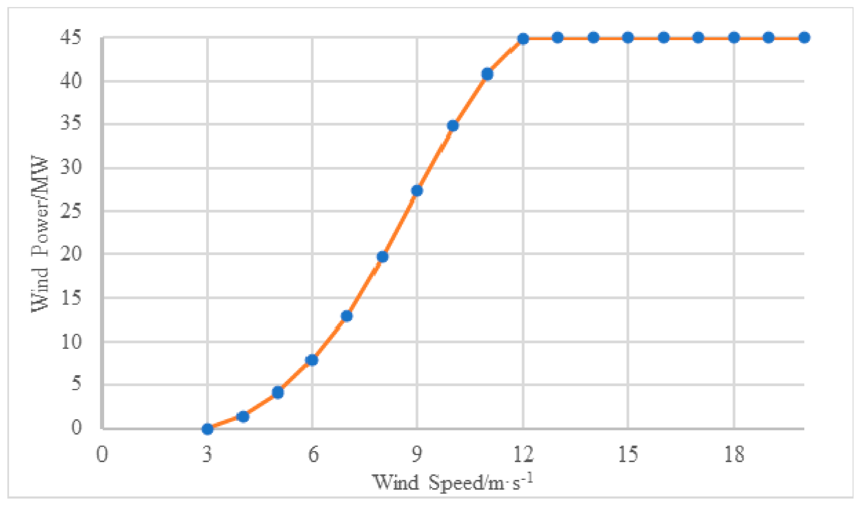
Figure 2 shows the relationship curve between theoretical wind power and wind speed. The curve expression can be obtained by Fourier fitting:
f ( v 0 ) = 28.56 10.42 c o s ( ω v 0 ) 20.99 s i n ( ω v 0 ) + 2.651 c o s ( 2 ω v 0 ) 6.133 s i n ( 2 ω v 0 ) 1.31 c o s ( 3 ω v 0 ) 2.363 s i n ( 3 ω v 0 ) + 0.029 c o s ( 4 ω v 0 ) 1.321 s i n ( 4 ω v 0 ) 0.3 c o s ( 5 ω v 0 ) 0.386 s i n ( 5 ω v 0 )
The value range of v0 can be obtained in the formula 3   m / s v 0 25   m / s according to its entry and exit wind speed.
By substituting Equation (5) into Equation (4) and taking the limit of the noise element value, the expression of the upper and lower envelope can be obtained [21]:
{ P 1 ( v 0 ) = f ( v 0 ) + a f ( v 0 ) + b f ( v 0 ) P 2 ( v 0 ) = f ( v 0 ) a f ( v 0 ) b f ( v 0 )
P1 represents the upper envelope of theoretical wind power, P2 represents the lower envelope of theoretical wind power, and a and b represent the differential coefficients after expansion.
By changing the values of a and b, the expression of the upper and lower envelope was calculated as the confidence interval, the confidence degree α within the interval was calculated, and the data outside the interval were taken as the wrong power data caused by the system false positive and other reasons. Confidence α is defined as
α = N C N T
NC refers to the number of data within the confidence interval, and NT refers to the total data.
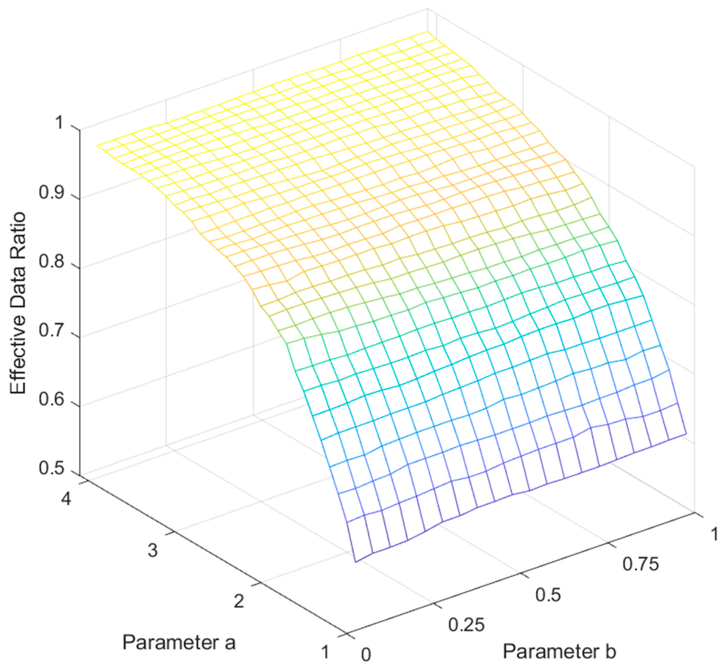
Figure 3 shows the changes in confidence when parameters a and b vary within the range [1, 4] and [0, 1], respectively. As seen from Figure 3, when and b > 0.6 , the confidence will increase, but the increase is slight and will lead to more severe distortion of the fitting curve, so a = 2.3, b = 0.51, and confidence α = 0.8917 .

3.1.2. Model Optimization

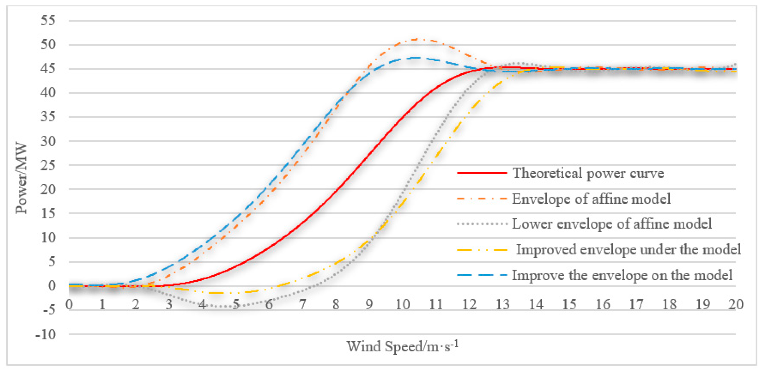
As can be seen from Figure 4 and basic mathematical theory, when the sine function is superimposed with its higher derivative, crest superposition will occur, resulting in curve protrusion, which will make it deviate significantly from the theoretical power curve. According to the mathematical knowledge, the superposition of higher derivatives based on the original model can realize the cancellation of sine function peaks and valleys. Then the optimized model can be obtained:
{ P 1 ( v 0 ) = f ( v 0 ) + a f ( v 0 ) + b f ( v 0 ) + c f ( v 0 ) P 2 ( v 0 ) = f ( v 0 ) a f ( v 0 ) + b f ( v 0 ) c f ( v 0 )
The coefficients a = 2.3, b = 2, and c = 0.8 were determined by the same method, and the confidence α = 0.9271. Figure 4 compares the upper and lower envelope before and after the improved model. It can be seen from the figure that the improved curve is more similar to the theoretical curve than the pre-improved curve, and the confidence value is more significant under the same conditions.
The data outside the envelope are screened out and corrected based on historical data. First, cluster the historical data and divide the similar data of wind speed, temperature, humidity, and air pressure. For the data outside the envelope, a similar class of historical data are taken for transfer learning and data correction.

3.2. PSO-SWLSTM Prediction Model of Wind Power

3.2.1. Model Introduction

This paper proposes a self-moving window long- and short-term memory neural network prediction model based on particle swarm optimization (PSO-SWLSTM). That is to say, particle swarm optimization is used to optimize the SWLSTM model learning rate and hidden layer element number parameters. At the same time, the traditional LSTM model is improved using a self-moving window. The model is enhanced and optimized based on the conventional LSTM model, so it is good at dealing with long-term dependence and complex nonlinear problems. The critical parameters of the SWLSTM model are optimized by the PSO algorithm based on an adaptive learning strategy to match the data characteristics with the network topology structure and improve the prediction accuracy [22]. At the same time, a self-moving window is adopted to realize gradual prediction by setting the window length, which is more consistent with the relationship between wind power and time, to improve the prediction accuracy.
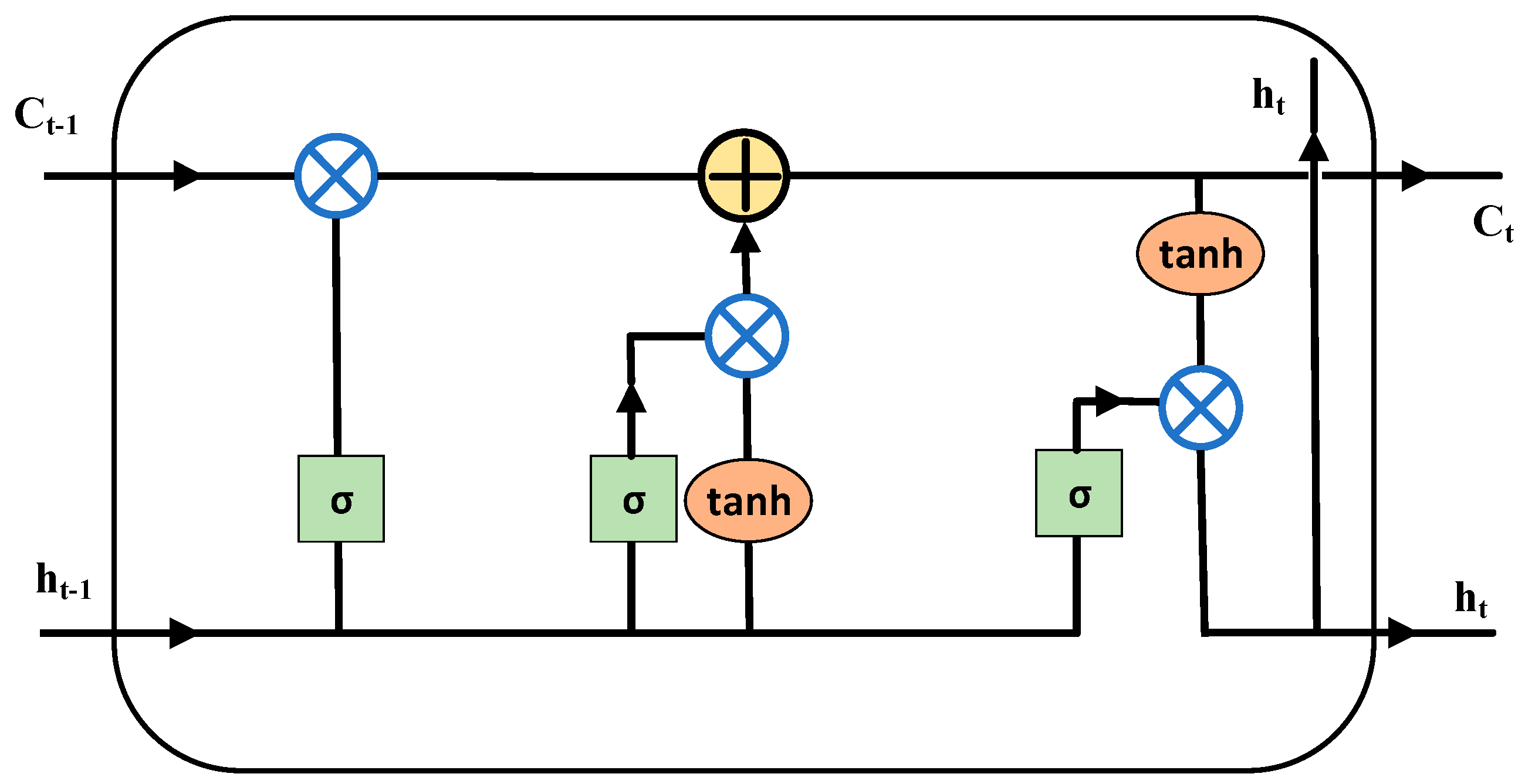
The LSTM model can solve the problems of gradient explosion, gradient disappearance, and the inability to preserve historical information in the long time series training process of the cyclic neural network (RNN). The LSTM model can provide better prediction performance in more comprehensive historical data than traditional cyclic neural networks. The interior of the LSTM consists of three unique gate structures and a status module for storing memories [23]. The cell structure of the LSTM is shown in Figure 5.
The three control gates in the memory unit are the input gate, the forgetting gate, and the output gate. The input gate can determine the information to be stored in the unit according to the conditions. The forgetting gate is used to retain the historical status information of the team. In addition, the output gate is used to control the output of data. A status module refers to the Sigmoid activation function, which can map the outcome of the control gate to the interval [0, 1]. The closer the value is to 1, the more information is retained. When the value is 0, the data are forgotten [24]. The following formula can describe the principle of traditional LSTM:
{ f t = S i g m o i d ( ω f [ h t 1 m t ] + b f ) i t = S i g m o i d ( ω i [ h t 1 m t ] + i ) C t = S i g m o i d ( ω C [ h t 1 m t ] + b C ) C t = f t × C t 1 + i t × C t O t = S i g m o i d ( ω O [ h t 1 m t ] + b O ) h t 1 = O t × t a n h ( C t )
where t represents the current moment and t − 1 represents the last moment; mt represents the input vector at this point; ht−1 represents the output vector of the hidden layer at the earlier time; ft, it, and Ot represent the forgetting gate, input gate, and output gate, respectively; ωf, ωi, and ωO represent the weights of the overlooked, input, and output gates, respectively; bf, bi, and bO represent the offset of the forgetting gate, input gate, and output gate, respectively. C t Ct′ stands for candidate state; Ct represents the calculated new state.
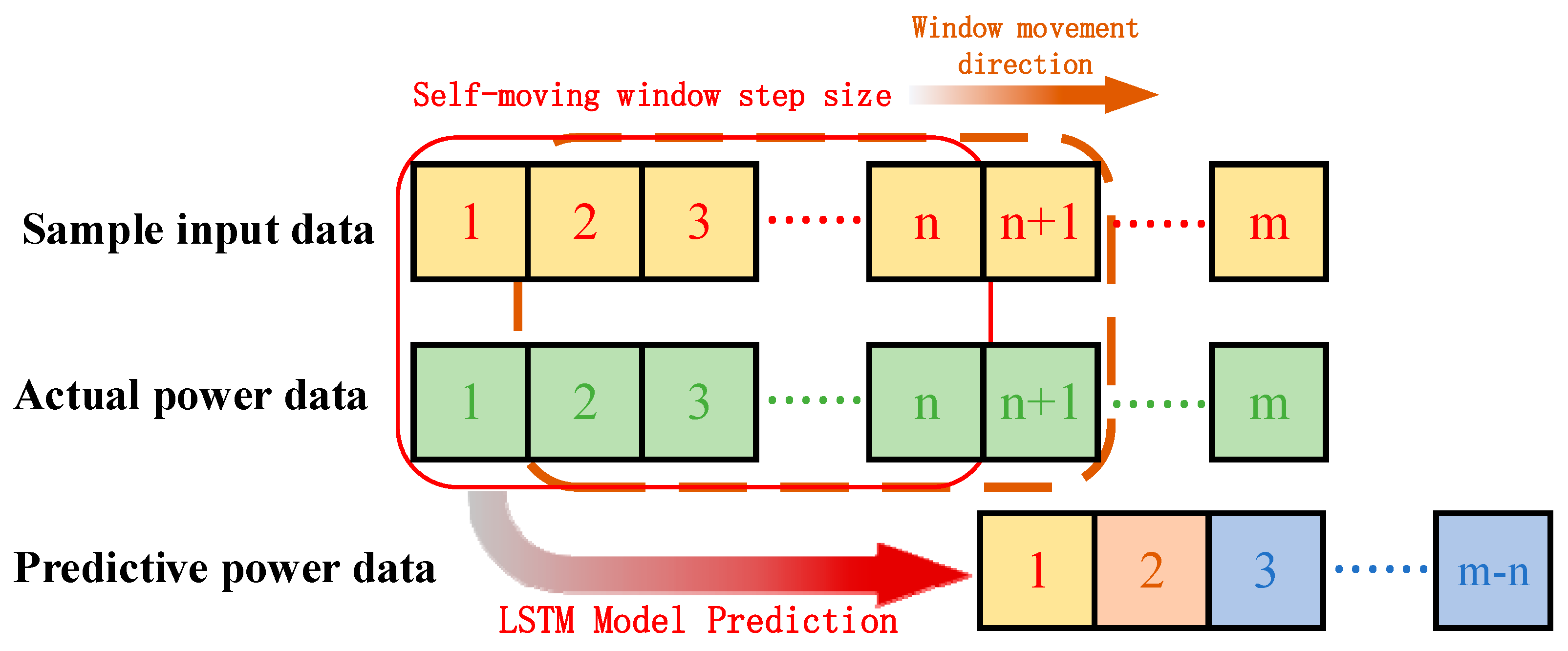
The SWLSTM model proposed in this paper is based on the traditional LSTM model. By setting the step size of the self-moving window, the training and prediction of the conventional LSTM model are changed to the gradual forecast along with the window movement. The prediction process of the SWLSTM model is shown in Figure 6. Determine the data length in a window by creating a self-moving window and setting its step size. Then, it was put into the LSTM model, the characteristics of the input data were extracted, the relationship between input meteorological element data and power data was trained, and the prediction model was established. Conclusively, realize the prediction of the following step data. The control window moves to the right step by step to complete the projection of power data and a perfect prediction model network is obtained. Compared with the traditional LSTM model, SWLSTM can shorten the length of the initial training step to extract more feature information and retain the data features more clearly. Therefore, the PSO-SWLSTM model can improve the prediction accuracy of wind power.

3.2.2. Simulation Steps and Parameter Settings

The process of the PSO-SWLSTM is as follows:
(1)
Normalize the processed data to facilitate subsequent data processing and map the data to 0~1 for processing.
(2)
Select the hyperparameters (number of neurons and learning rate) that need to be adjusted in LSTM and their respective optimization ranges.
(3)
Initialize PSO parameters. This includes the initial velocity, position, training frequency, and particle scale. The number of particle training is set to 20, and the number of particles is set to 100.
(4)
Set the inertia weight of PSO as 0.8 to ensure faster convergence speed of the particle swarm optimization algorithm.
(5)
Determine the fitness function of particles. In this paper, the RMSE value of the SWLSTM prediction model will be minimized as the fitness function of particles, and the optimal model parameters will be sought.
(6)
Set the step size of the model’s self-moving window. The SWLSTM model takes an eight step size as the window to predict step by step.
(7)
Calculate the fitness value of particles and update the optimal fitness value.
(8)
Record the optimal position of particles and update the optimal part of the population.
(9)
Determine whether the number of cycles is reached. If the number of cycles is satisfied, the optimal position of the particle swarm and SWLSTM prediction results are output. If not, return to Step 7.
The root mean square error RMSE of the electrical industry standard stroke power prediction reflects the pros and cons of wind power prediction results and is defined as:
R M S E = i = 1 n ( P Mi P Pi ) 2 C a p n × 100 %
where PPI is the predicted power at the time i, PMi is the actual power at the time i, Cap is the total start-up capacity of the wind farm, and n is the number of all samples.
In this paper, mean absolute percentage error MAPE is adopted to measure the statistical index of wind power prediction accuracy, which is defined as:
M A P E = 100 % n i = 1 n | P Mi P Pi P Mi |
The fitness function in the particle swarm optimization algorithm is defined to minimize the predicted root mean square error RMSE. Its constraint function includes the position limit of particles (i.e., the learning rate of each particle and the implied unit number limit) and the speed limit of particles (i.e., the range of movement limit of each particle during iteration). The particle swarm optimization model is defined as follows.
min f ( x ) = R M S E s . t . 10 5 x learn 0.01      1 x unit 64     0.005 v learn 0.005     1 v unit 1
where xlearn and vlearn, respectively, refer to the position and speed of the particle learning rate, and xunit and vunit, respectively, refer to the place and pace of the particle implied unit number.

3.3. Wind Power Error Feedback Correction Model Based on LSTM

3.3.1. Model Introduction

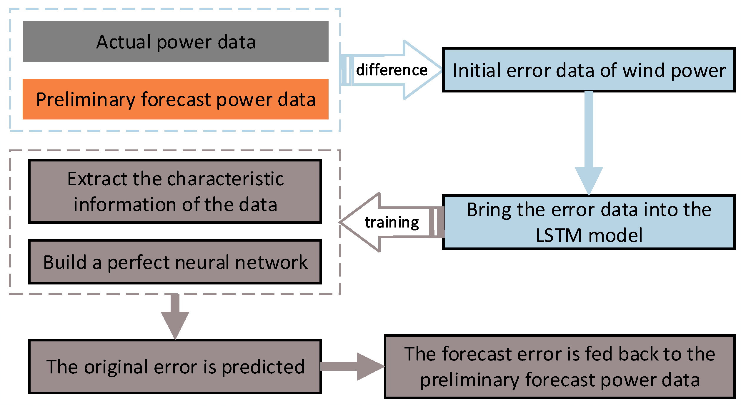
This paper proposes an error feedback correction model (EFCM-LSTM) based on the LSTM network. The error between the predicted data and the actual power data of PSO-SWLSTM is calculated. Then, the error is input into the LSTM prediction model as input data to realize the error prediction. Then, the preliminary forecast data of PSO-SWLSTM are revised. By predicting the error data, the error caused by the initial prognosis is offset to improve the prediction accuracy.
The schematic diagram of the EFCM-LSTM model proposed in this paper is shown in Figure 7. The PSO-SWLSTM model predicts the power data of the preliminary prediction, and the error between the expected power data and the actual power is calculated, which is input into the LSTM model together with the meteorological factor data. The LSTM model is used to extract the characteristics of the errors and meteorological data and establish the relationship network. The output data of the LSTM model are the predicted data of the error, which is returned to the power data indicated by the PSO-SWLSTM model, and the corrected power data are finally obtained.
Considering that the time step of short-term prediction is generally tens of degrees and the time step predicted in this paper is 40 steps, the time series of wind power has a more significant correlation with the error data. Suppose the SWLSTM model is used to predict the error. In that case, the influence of time characteristics on the error series is challenging to consider thoroughly, and the time of model training prediction will increase. Therefore, the LSTM model is adopted in this paper for error prediction correction.
To evaluate the merits of the prediction results and the final corrected power data, root means the square error was introduced to quantify the effects, which were defined as follows:
R M S E err = i = 1 n ( P EMi P EPi ) 2 C a p n × 100 % R M S E P = i = 1 n ( P RMi P RPi ) 2 C a p n × 100 %
where PEPi is the error power predicted at the time i, PEmi is the original error power at the time i, PRPi is the expected power corrected at the time i, PRMi is the actual original power at the time i, Cap is the total start-up capacity of the wind farm, and n is the number of all samples.

3.3.2. Simulation Process and Parameter Setting

First of all, the 960 sample data should be divided into three groups: A, B, and C, and the quantity ratio of the three groups is 3:2:1. Group A is used as the training group of the PSO-SWLSTM prediction model, group B is used as the training and testing group of EFCM-LSTM correction model, and group C is used as the EFCM-LSTM model test group.
A group of data were used to train the PSO-SWLSTM model. Meteorological factors and power data were input into the PSO-SWLSTM model as input data for extracting feature information and establishing a prediction network. The output data were the predicted value of the power data, and the root means square error RMSE of predicted power and actual power was calculated. The model parameters of PSO-LSTM are consistent with those in Section 3.2. Group B’s meteorological factors and power data are brought into the prediction network trained by group A data as input data. The predicted power data of group B data are obtained, and the difference between the expected power data of group B and the actual power data is calculated as the initial error data. The meteorological factor data and error data of group B data were input into the LSTM model as input data to establish the error prediction network. The relevant parameters of the LSTM model are set as follows: the training cycle is 400, the learning rate is 0.001, and the number of hidden units is 16. Group C, as the test group, inputs the meteorological factor data and power data into the network of group A to obtain the preliminary forecast power and calculate the original error data. Then, input the error data and meteorological data into the web of group B to obtain the forecast error data, and finally, calculate the corrected power data with the preliminary forecast power data.

4. Model Simulation and Result Analysis

This paper uses an example of a wind farm in East China to simulate the model and forecast the wind power for ten hours. The data set includes NWP data of the wind farm in 2020 and historical wind power data, with a time resolution of 15 min. The data from 10 days were selected as the simulation data set, namely 960 sample data.

4.1. Affine Optimization Model Results

The affine optimization model is an approximate curve obtained by mathematical transformation according to the fitting curve. Considering the characteristics of the sine function, the amplitude fluctuation of the affine optimization curve is smaller than that of the theoretical curve, which is a normal phenomenon. This paper considers only the confidence interval composed of the affine optimization curve for data screening and correction.
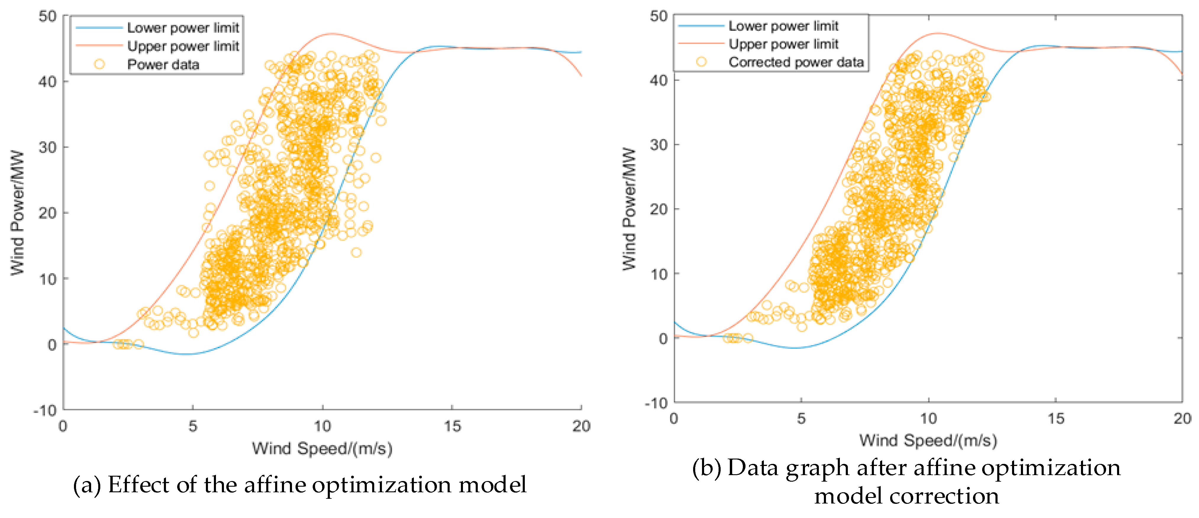
Figure 8a is the model effect diagram of the affine optimization curve and wind power data. It can be seen from the figure that most power data are located in the confidence interval composed of the affine optimization curve. In addition, the confidence degree of the affine optimization curve in the figure is 92.71%, which means that the power data within the confidence interval is considered to meet the requirements. The power data outside the confidence interval are deemed false positives that must be corrected.
The affine optimization model screens the error data, and the mean value of the data with similar conditions is found in the historical data according to the meteorological factor data corresponding to the error data as correction data. First, it is necessary to normalize wind speed data of 10 m, 30 m, 50 m, and 70 m and meteorological data of air pressure, temperature, and humidity. The condition is ±5% of the meteorological data corresponding to the incorrect data. Using the idea of learning transfer, the mean value of power data with similar meteorological conditions in the historical data is found as the correction data.
Figure 8b shows the power data graph after affine optimization model correction. The corrected data are all within the confidence interval, and the correlation between the power data and the theoretical power is better, which makes the feature information between the model prediction and data extraction in the next step more abundant and more accessible.

4.2. Parameter Optimization Result

Particle swarm optimization is a heuristic stochastic optimization algorithm. The optimization of each generation is the global optimization of the objective function, and the optimization results may be different each time, which is also a normal phenomenon of the heuristic optimization algorithm. This paper uses the particle swarm optimization algorithm to improve the SWLSTM neural network. By using the global optimization ability of the particle swarm optimization algorithm, the learning rate and the number of hidden units in the SWLSTM model are globally optimized. Therefore, the average value of the ten optimization results is taken as this paper’s final parameter optimization value to obtain the optimal parameter.
For the average values of the optimization results of relevant parameters obtained after ten pieces of training, the learning rate of the SWLSTM model is 0.0054 and the number of hidden units is 48.

4.3. Comparative Analysis of Prediction Results

To verify the effectiveness of the model proposed in this paper, four models, M1, M2, M3, and M4, are selected as the reference models for comparison, as shown in Table 1. Table 2 is a descriptive analysis table of relevant parameters of the data set in this paper. Including wind speed, pressure, humidity, temperature and power maximum value, mean value, skewness, kurtosis, and other information.
Table 3 shows the RMSE value of the five models for ten times of prediction and the average RMSE value of each model for ten times of prophecy. It can be seen from the data in the table that the prediction error of the model in this paper is smaller than that of the other four models for each wind farm. Because the proposed model uses two kinds of neural network models to make superposition predictions, the prediction error is reduced compared with other mainstream methods. The advantages of the two neural networks are utilized to play an essential role in the prediction and error correction process. At the same time, this reason also leads to the instability of the model. The mean value of the root means square error RMSE is 9.058% when this model predicts wind power. The mean square error RMSE of the M1, M2, M3, and M4 models are 19.759%, 16.048%, 13.862%, and 13.516%, respectively.
At the same time, a new evaluation index, RMSEDi%, is added to describe the accuracy improvement after the error correction at step i to evaluate the model’s accuracy more intuitively. RMSEDi% is defined as follows:
R M S E Di % = ( R M S E av   i - 1 R M S E av   i ) R M S E av   i - 1 × 100 %
RMSEav i is the mean value of the RMSE predicted results after error correction at step i, and RMSEav 0 represents the mean value of RMSE predicted by the traditional LSTM model.
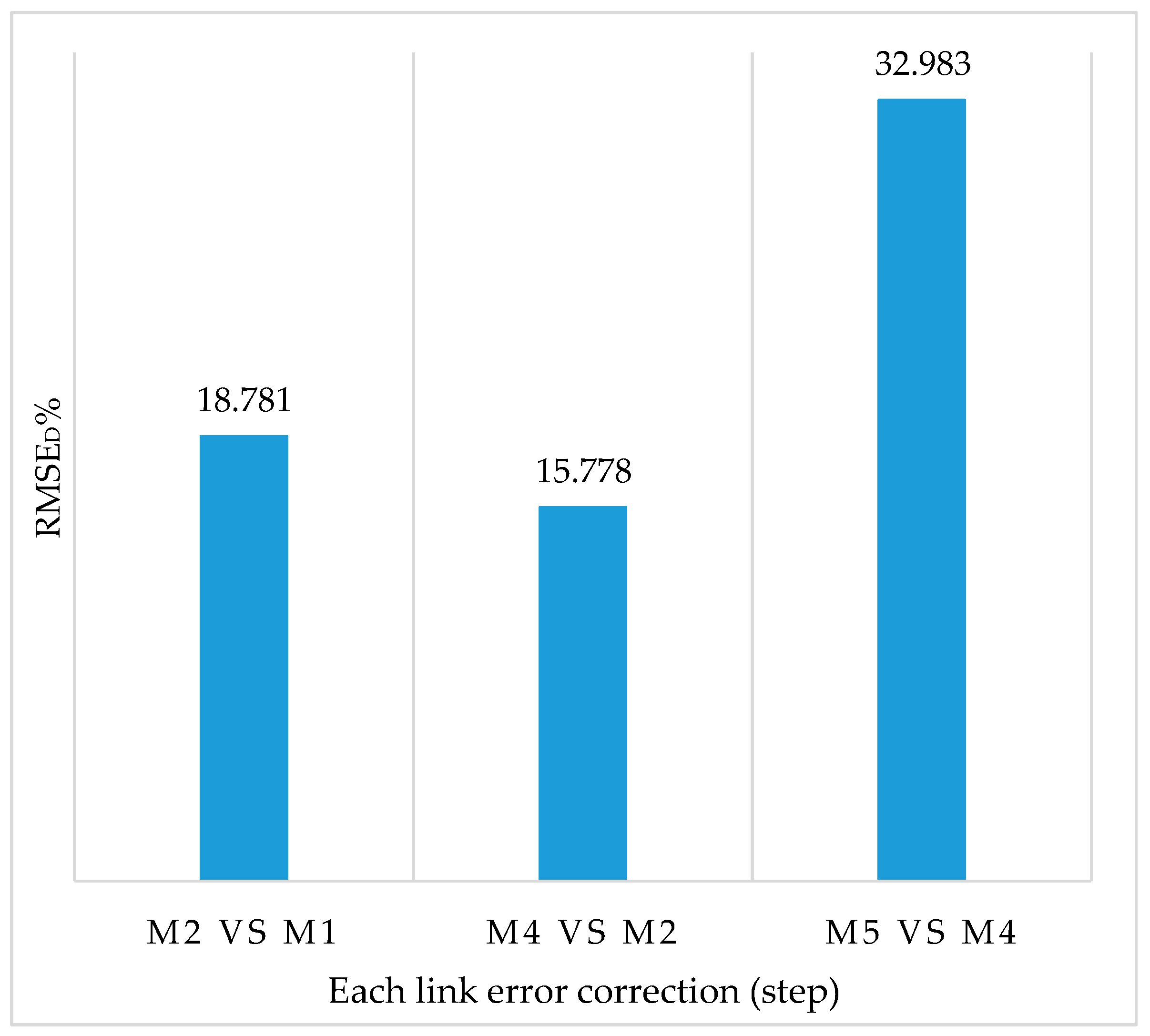
After calculation, the percentage increase of RMSE after three-step error correction was obtained, and the bar chart was drawn, as shown in Figure 9.
As can be seen from the figure, when only the PSO-SWLSTM model is used for power prediction, the error of the model is reduced by 18.781% compared with the traditional LSTM model. After modifying the original data by affine optimization model, the PSO-SWLSTM model is used for prediction, and the model error is reduced by 15.778% compared with only using the PSO-LSTM model. After adding the EFCM-LSTM model for feedback correction of prediction error, the RMSE of the model was reduced by 32.983% compared with the previous step.
Table 4 shows the MAPE values of the ten predicted results and the average MAPE values of the ten anticipated results during each model’s prediction. As seen from the data in the table, the prediction results of the model proposed in this paper are better than other standard models.
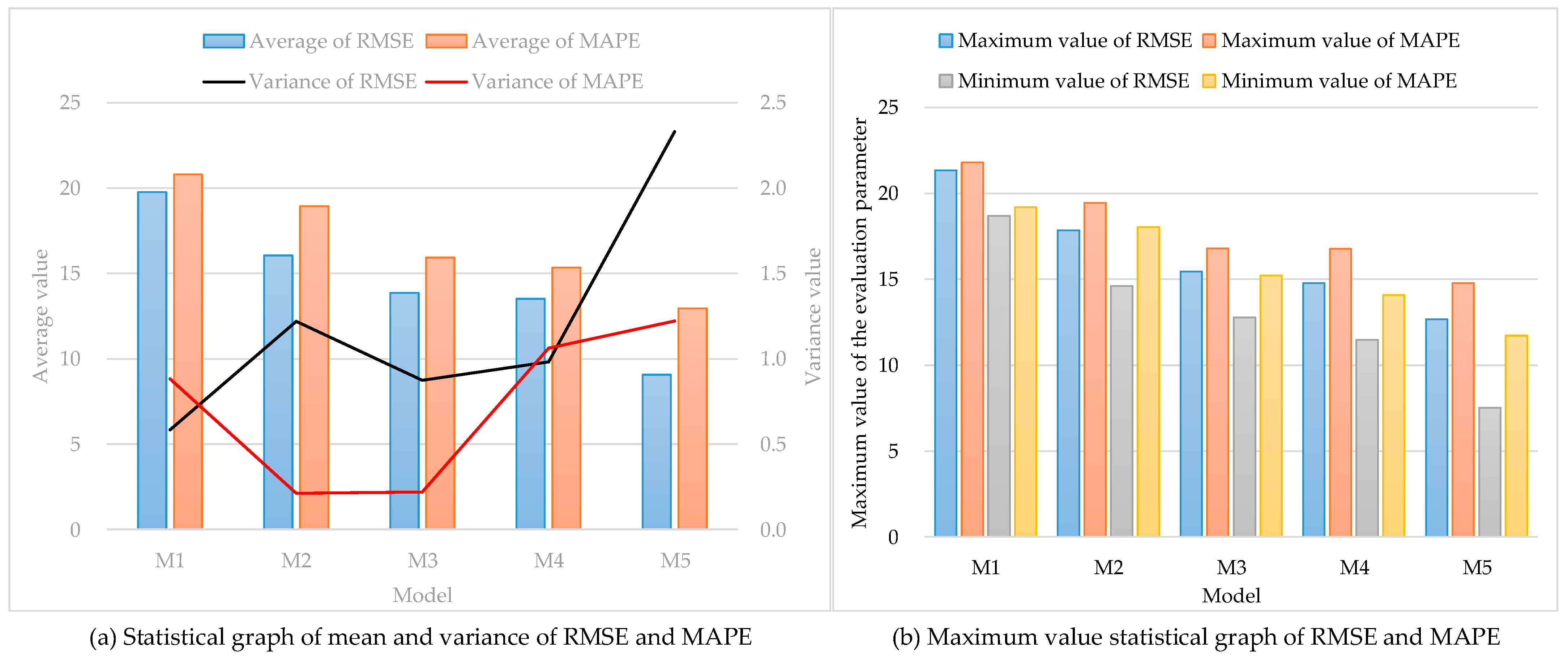
Figure 10a shows the mean and variance of RMSE and MAPE for ten predictions of the five models. Figure 10b shows the maximum values of RMSE and MAPE for the results of 10 predictions of the five models. Combined with the two figures, it can be seen that the model proposed in this paper (M5) can effectively reduce the prediction error, and the mean values of RMSE and MAPE are lower than those of the other four models. However, the variance of RMSE and MAPE is high, indicating that the model proposed in this paper has high volatility, but their conflict is controlled at about 1. The maximum value of RMSE and MAPE of the predicted data was within 15%, and the mean value was 10%. Even though the stability was poor, it could still maintain good prediction performance compared with other models.
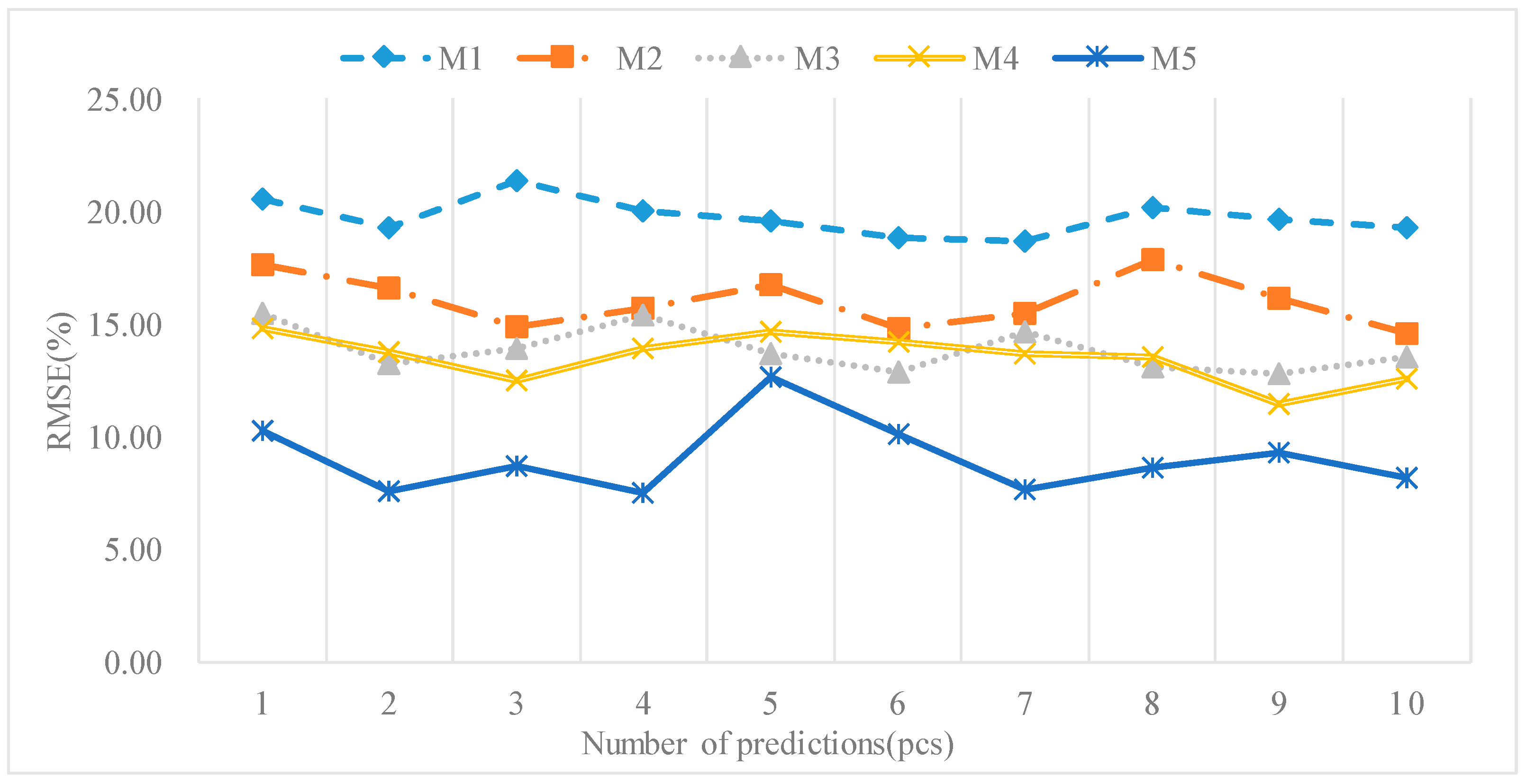
Figure 11 shows the root mean square error pattern of the ten times model training prediction results. The following conclusions can be drawn through the analysis of Figure 11:
(1)
Compared with the traditional LSTM model, the PSO-SWLSTM model proposed in this paper can reduce the root mean square error of prediction results and obtain more reasonable predictions.
(2)
We can see that by comparing M3 and M4 curves with the M1 curves. The affine optimization model and EFCM-LSTM model proposed in this paper can effectively reduce the error of prediction results in data correction or error correction. This makes the forecast more efficient and reasonable.
(3)
It can be seen from the observation curves M3 and M4 that the improved model has good stability, and the RMSE value of the predicted result is stable at about 15%, which can improve the model prediction result stably and effectively.
(4)
Compared with the traditional LSTM model, the model proposed in this paper can significantly improve the prediction results and control the RMSE value at about 10%. The best result in 10 training can reach 7.52%.
The model presented in this paper uses the PSO-SWLSTM model for prediction and the EFCM-LSTM model for prediction error correction. That is to say, the proposed model carries out two forms of neural network information extraction and model training. Compared with this paper, the other model only carries out one form of neural network training and learning. As there are certain uncertainties and unstable factors in the training of the neural network model each time, the RMSE value of the predicted results of the proposed model in this paper will fluctuate.
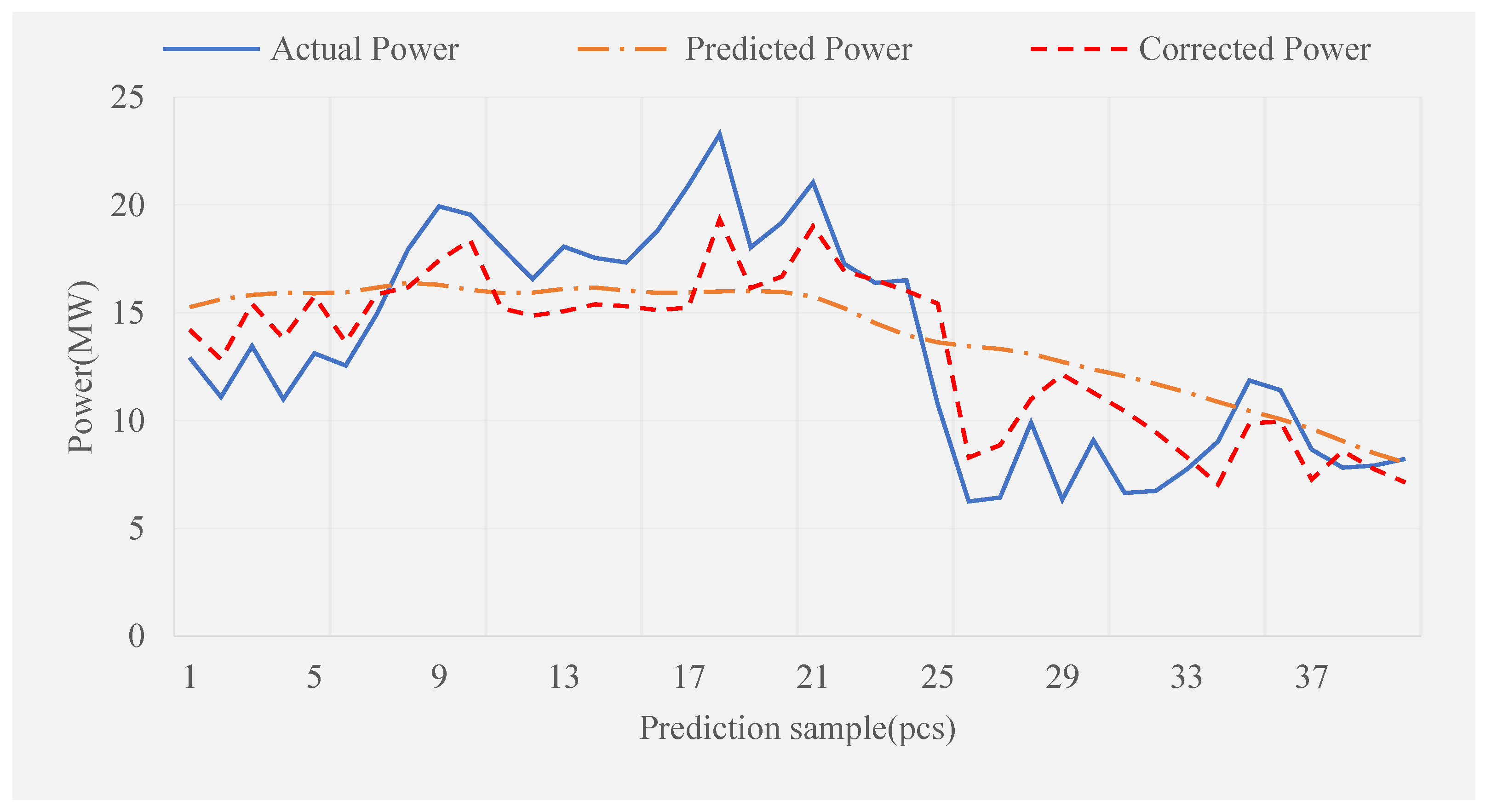
Figure 12 shows the prediction and correction data of the model proposed in this paper. The predicted data is the expected power obtained after sample correction by affine optimization model data after PSO-LSTM model training. The updated power data are the corrected data obtained after the prediction error is introduced into the EFCM-LSTM model. As seen from the figure, the model-predicted power data before correction cannot clearly show the trend and fluctuation of the actual power. After modification, the movement and change of true power can be reflected.
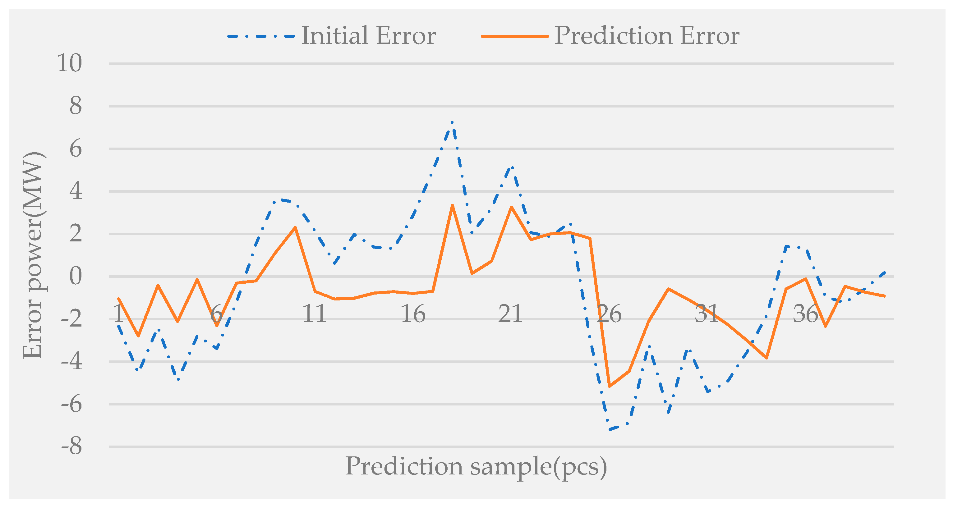
Figure 13 shows the trend chart of error data after the initial error prediction by the EFCM-LSTM model. It can be seen from the figure that EFCM-LSTM can remarkably restore the error fluctuation of original data, which indicates that correction of prediction error has excellent advantages in the field of short-term wind power prediction.

5. Conclusions

As the proportion of installed wind power capacity increases year by year, short-term wind power forecast plays an essential role in the safe operation of power systems and the rational scheduling of wind power generation. This paper presents a multi-error correction short-term wind power LSTM prediction method.
(1) Compared with the traditional LSTM model, the improved LSTM model with a self-moving window can obtain more accurate short-term wind power prediction results. This shows that adding the self-moving window method can enrich the feature information extracted by the neural network and build a perfect network system. Thus, the prediction accuracy can be effectively improved.
(2) In this paper, an affine optimization model is used for data screening, and a learning transfer idea is used for data correction. After preliminary prediction, the LSTM model is used to predict further predicted power errors, and conclusively, the corrected power data is obtained. The results show that data and prediction error correction can effectively improve prediction accuracy.
(3) In this paper, the particle swarm optimization algorithm is used to optimize the parameters of the LSTM model based on the self-moving window. The particle swarm optimization algorithm optimizes the learning rate and the number of hidden units in the SWLSTM model. The results show that the improved algorithm can obtain the model parameter combination that minimizes the RMSE value, thus improving the model’s prediction accuracy.
This model predicts that the system’s safety, reliability, and controllability can be enhanced according to the variation law of wind power output, and the operation cost of the power system can be reduced. The improvement of wind power prediction accuracy is of great significance to reduce carbon emissions, accelerate carbon neutrality, gradually replace thermal power generation, and simultaneously meet the sustainable development trend of the international community.

Author Contributions

The authors confirm their contributions to the paper as follows: conceptualization, F.T. and Z.X.; methodology, F.T., M.W. and Z.X.; validation, Z.X. and M.W.; resources, F.T.; data curation, F.T.; writing—original draft preparation, Z.X.; writing—review and editing, F.T. and Z.X.; supervision, F.T.; project administration, F.T. All authors have read and agreed to the published version of the manuscript.

Funding

This paper study was funded by the National Natural Science Foundation of China (Grant number 51977157).

Institutional Review Board Statement

Not applicable.

Informed Consent Statement

Not applicable.

Data Availability Statement

The data came from a wind farm in the south of the Grid Company’s cooperative project, which was obtained through project cooperation. Because of the confidentiality agreement, the specific name of the wind farm, latitude and longitude information, and data information cannot be disclosed. Necessary cleaning and desensitization of data have been carried out in the process of writing the paper, which can be used for scientific research exchange without legal affairs and intellectual property rights problems.

Conflicts of Interest

The authors declare no conflict of interest.

Nomenclature

IEEEInstitute of Electrical and Electronics Engineers
PSO-SWLSTMSelf-moving window long and short-term memory neural network prediction model based on particle swarm optimization
EFCM-LSTMError feedback correction model based on the LSTM network
MWMegawatt
p. u.Per unit
pcsPieces
ρRepresents the correlation between meteorological factors and wind power
xtTime series data of meteorological factors
ytTime series data of wind power
X ¯ The mean of the time series of meteorological factors
Y ¯ The mean value of wind power time series
V10Wind speed 10 m above the ground at any given time
V30Wind speed 30 m above the ground at any given time
V50Wind speed 50 m above the ground at any given time
V70Wind speed 70 m above the ground at any given time
TThe temperature of the atmosphere at a given time
FThe humidity of the atmosphere at a given time
PAtmospheric pressure at a given time
ε1Noise element introduced by prediction error.
ε2Noise elements are introduced by other factors affecting the calculation error of wind speed.
x1, x2The noise element coefficient reflects the degree to which the corresponding noise element causes the input wind speed to deviate from the predicted wind speed.
P1The upper limit power of the wind power affine model
P2The lower limit power of the wind power affine model
P3The upper limit power of an affine optimization model for wind power
P4The lower limit power of an affine optimization model for wind power
a, b, c, dDifferential coefficient of the affine model after Taylor expansion
αThe ratio of the number of data in the confidence interval to the number of all data
ft, it, OtRespectively represent the forgetting gate, input gate, and output gate.
ωf, ωi, ωORespectively represent the weight of the forgetting, input, and output gates.
mtRepresents the input vector of the LSTM model at time t
ht−1Represents the output vector of the hidden layer of the LSTM model at time t − 1
RMSERoot mean square error of wind power prediction
RMSEerrThe root means a square error of the error data.
RMSCorrect root means a square error of power data.
PPIPredicted power at time i
PEPiError power predicted at time i
PRPiPredicted power after correction at time i
PMiThe actual power at time i
PEMiThe original error power at time i
PRMiThe actual original power at time i
CapTotal start-up capacity of the wind farm
xlearn, vlearnRefer to the position and speed of particle learning rate, respectively
xunit, vunitRefer to the position and velocity of the number of implied units of a particle, respectively

References

  1. Dong, Z.; Wong, K.P.; Meng, K.; Luo, F.; Yao, F.; Zhao, J. Wind power impact on system operations and planning. In Proceedings of the IEEE PES General Meeting, Minneapolis, MN, USA, 25–29 July 2010; IEEE: Piscataway, NJ, USA, 2010; pp. 1–5. [Google Scholar]
  2. He, Q.; Chen, H.; Lin, Z.; Dai, X.; Huang, Y.; Cai, W. A cost-based life-cycle pricing model for offshore wind power plants within China’s carbon trading scheme. Energy Rep. 2022, 8, 147–155. [Google Scholar] [CrossRef]
  3. Wang, J.; Zhou, Y. Multi-objective dynamic unit commitment optimization for energy-saving and emission reduction with wind power. In Proceedings of the 2015 5th International Conference on Electric Utility Deregulation and Restructuring and Power Technologies (DRPT), Changsha, China, 26–29 November 2015; IEEE: Piscataway, NJ, USA, 2015; pp. 2074–2078. [Google Scholar]
  4. Bokde, N.; Feijóo, A.; Villanueva, D.; Kulat, K. A Review on Hybrid Empirical Mode Decomposition Models for Wind Speed and Wind Power Prediction. Energies 2019, 12, 254. [Google Scholar] [CrossRef] [Green Version]
  5. Lu, P.; Ye, L.; Zhao, Y. Review of meta-heuristic algorithms for wind power prediction: Methodologies, applications, and challenges. Appl. Energy 2021, 301, 117446. [Google Scholar] [CrossRef]
  6. De Giorgi, M.G.; Ficarella, A.; Tarantino, M. Error analysis of short-term wind power prediction models. Appl. Energy 2011, 88, 1298–1311. [Google Scholar] [CrossRef]
  7. Shahid, F.; Zameer, A.; Muneeb, M. A novel genetic LSTM model for wind power forecast. Energy 2021, 223, 120069. [Google Scholar] [CrossRef]
  8. Hu, Y.-L.; Chen, L. A nonlinear hybrid wind speed forecasting model using LSTM network, hysteretic ELM, and Differential Evolution algorithm. Energy Convers. Manag. 2018, 173, 123–142. [Google Scholar] [CrossRef]
  9. Chen, M.-R.; Zeng, G.-Q.; Lu, K.-D.; Weng, J. A two-layer nonlinear combination method for short-term wind speed prediction based on ELM, ENN, and LSTM. IEEE Internet Things J. 2019, 6, 6997–7010. [Google Scholar] [CrossRef]
  10. Wang, X.; Li, J.; Shao, L.; Liu, H.; Ren, L.; Zhu, L. Short-Term Wind Power Prediction by an Extreme Learning Machine Based on an Improved Hunter–Prey Optimization Algorithm. Sustainability 2023, 15, 991. [Google Scholar] [CrossRef]
  11. Zhang, Z.; Wang, J.; Wei, D. A novel ensemble system for short-term wind speed forecasting based on Two-stage Attention-Based Recurrent Neural Network. Renew. Energy 2023, 204, 11–23. [Google Scholar] [CrossRef]
  12. Jaseena, K.; Kovoor, B.C. Decomposition-based hybrid wind speed forecasting model using deep bidirectional LSTM networks. Energy Convers. Manag. 2021, 234, 113944. [Google Scholar] [CrossRef]
  13. Liu, H.; Mi, X.; Li, Y. Smart multi-step deep learning model for wind speed forecasting based on variational mode decomposition, singular spectrum analysis, LSTM network, and ELM. Energy Convers. Manag. 2018, 159, 54–64. [Google Scholar] [CrossRef]
  14. Zhou, J.; Yu, X.; Jin, B. Short-Term Wind Power Forecasting: A New Hybrid Model Combined Extreme-Point Symmetric Mode Decomposition, Extreme Learning Machine and Particle Swarm Optimization. Sustainability 2018, 10, 3202. [Google Scholar] [CrossRef] [Green Version]
  15. Sheng, Y.; Wang, H.; Yan, J. Short-term wind power prediction method based on deep clustering-improved Temporal Convolutional Network. Energy Rep. 2023, 9, 2118–2129. [Google Scholar] [CrossRef]
  16. Cali, U.; Sharma, V. Short-term wind power forecasting using long-term memory-based recurrent neural network model and variable selection. Int. J. Smart Grid Clean Energy 2019, 8, 103–110. [Google Scholar] [CrossRef] [Green Version]
  17. Joseph, L.P.; Deo, R.C.; Prasad, R. Near real-time wind speed forecast model with bidirectional LSTM networks. Renew. Energy 2023, 204, 39–58. [Google Scholar] [CrossRef]
  18. Son, N.; Yang, S.; Na, J. Hybrid forecasting model for short-term wind power prediction using modified long short-term memory. Energies 2019, 12, 3901. [Google Scholar] [CrossRef] [Green Version]
  19. Shahid, F.; Zameer, A.; Mehmood, A. A novel wavenets long short-term memory paradigm for wind power prediction. Appl. Energy 2020, 269, 115098. [Google Scholar] [CrossRef]
  20. Zhang, J.; Yan, J.; Infield, D. Short-term forecasting and uncertainty analysis of wind turbine power based on long short-term memory network and Gaussian mixture model. Appl. Energy 2019, 241, 229–244. [Google Scholar] [CrossRef] [Green Version]
  21. Wu, J.H.; Shao, Z.G.; Yang, S.H. A combined algorithm for data cleaning of wind power scatter diagram considering actual engineering characteristics. IOP Publ. 2020, 1639, 012044. [Google Scholar] [CrossRef]
  22. Sun, Y.; Wang, X.; Yang, J. Modified Particle Swarm Optimization with Attention-Based LSTM for Wind Power Prediction. Energies 2022, 15, 4334. [Google Scholar] [CrossRef]
  23. Qu, J.Q.; Qian, Z.; Pei, Y. Day-ahead hourly photovoltaic power forecasting using attention-based CNN-LSTM neural network embedded with multiple relevant and target variables prediction pattern. Energy 2021, 232, 120996. [Google Scholar] [CrossRef]
  24. Wang, D.; Cui, X.; Niu, D. Wind Power Forecasting Based on LSTM Improved by EMD-PCA-RF. Sustainability 2022, 14, 7307. [Google Scholar] [CrossRef]
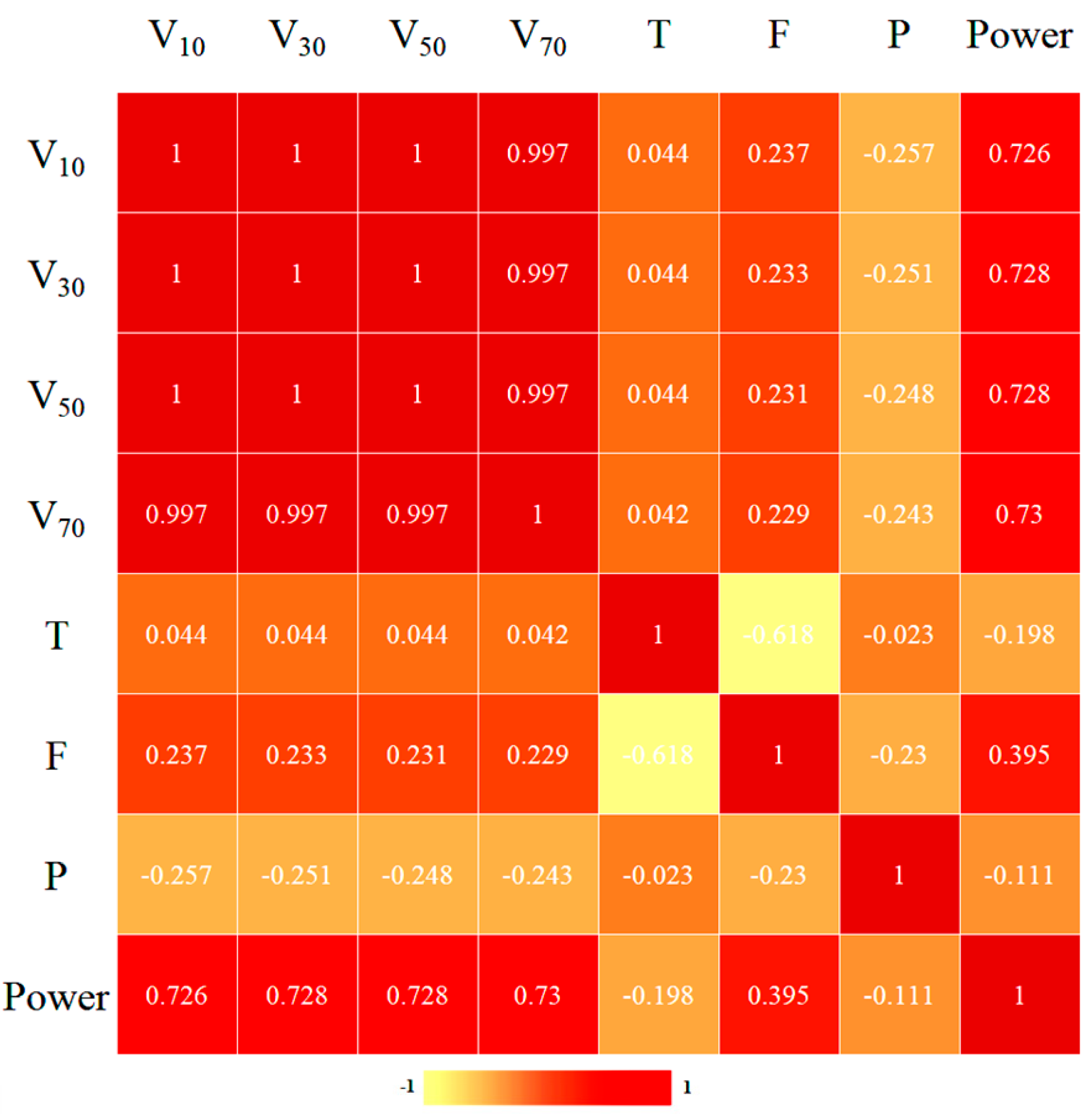
Figure 1. Correlation coefficient analysis heat map.
Sustainability 15 03798 g001
Figure 2. Theoretical wind power and wind speed curve.
Sustainability 15 03798 g002
Figure 3. The relationship of confidence with parameters a and b.
Sustainability 15 03798 g003
Figure 4. Comparison of the envelope before and after model improvement.
Sustainability 15 03798 g004
Figure 5. LSTM cell structure diagram.
Sustainability 15 03798 g005
Figure 6. SWLSTM prediction process diagram.
Sustainability 15 03798 g006
Figure 7. Diagram representing the process structure of the EFCM-LSTM model.
Sustainability 15 03798 g007
Figure 8. Comparison of the affine optimization model before and after correction.
Sustainability 15 03798 g008
Figure 9. Statistical chart of RMSED% analysis.
Sustainability 15 03798 g009
Figure 10. Descriptive statistical graph of each model’s prediction results.
Sustainability 15 03798 g010
Figure 11. RMSE data graph for ten times of model training.
Sustainability 15 03798 g011
Figure 12. Model prediction and correction results.
Sustainability 15 03798 g012
Figure 13. Prediction error data of the EFCM-LSTM model.
Sustainability 15 03798 g013
Table 1. Introduction to this paper model and other models.
ModelDescription of Model
M1The prediction using the traditional LSTM model
M2predicted by the self-moving window LSTM model (namely PSO-SWWLSTM) based on the particle swarm optimization algorithm.
M3The prediction using the PSO-SWWLSTM model, and the error feedback correction model based on the LSTM network (i.e., EFCM) is used to correct the predicted data.
M4The affine optimization model is first used for data correction, and then the PSO-SWLSTM model is used for prediction.
M5The model proposed in this paper.
Table 2. Statistical descriptions of the raw data sets.
CountMeanStandard DeviationMedianKurtosisSkewnessMinimumMaximum
Wind speed (10 m), m/s9606.2920.0436.330−0.085−0.1701.6009.280
Wind speed (30 m), m/s9607.3800.0507.420−0.124−0.1721.88010.860
Wind speed (50 m), m/s9607.9480.0547.990−0.141−0.1732.02011.690
Wind speed (70 m), m/s9608.3420.0578.395−0.114−0.1942.12012.260
Temperature, °C96027.7480.03927.54032.628−3.02914.46030.590
Humidity, %rh96087.4880.15188.195−0.104−0.48873.44096.370
Pressure, Pa9601003.0190.0851003.5381.781−1.403994.4631007.409
Wind power, MW96021.4780.36320.331−1.1190.187044.027
Table 3. RMSE values of each model prediction result.
ModelRMSE (%)
12345678910Average
M120.5719.3221.3520.0319.5618.8718.6920.2219.6719.3119.759
M217.6816.5814.8915.7316.7714.7915.4517.8516.1414.6016.048
M315.4513.2313.8915.4213.6712.8914.6313.1212.7813.5413.862
M414.7813.7612.4713.8914.6814.2513.6913.5711.4812.5913.516
M510.237.578.677.5212.6810.157.698.639.278.179.058
Table 4. MAPE values of each model prediction result.
ModelMAPE (%)
12345678910Average
M119.3520.6521.3521.8020.8719.1820.2221.4921.5821.4820.797
M219.0419.4519.0719.1218.0218.8018.9818.3319.4419.2618.951
M316.7915.4015.2215.6815.8916.3016.3216.1615.7315.8515.934
M416.6914.0814.4615.8815.0316.1914.4715.7116.7614.1715.344
M512.0313.0513.1811.9811.7214.7714.5713.1113.3711.7312.951
Disclaimer/Publisher’s Note: The statements, opinions and data contained in all publications are solely those of the individual author(s) and contributor(s) and not of MDPI and/or the editor(s). MDPI and/or the editor(s) disclaim responsibility for any injury to people or property resulting from any ideas, methods, instructions or products referred to in the content.