Stand Structure and Dynamics of the Naturally Managed Oak-Dominated Forests and Their Relation to Environmental Variables in Swat Hindu Kush Range of Pakistan

Abstract

Although oak woodlands are a characteristic landscape component in the Swat Hindukush Mountain ranges, little is known about their current or historical stand population structure and regeneration dynamics related to environmental variables. Therefore, the present study assessed the stand structure, regeneration status, and relationship of oak communities with environmental variables. The study assessed 30 oak-dominated forest sites using the quadrates method, sampling 300 quadrates for evaluating the phytosociological and environmental variables. The stand structures of forests were dominated by four oak species, i.e., Quercus incana, Quercus baloot, Quercus dilatata, and Quercus semecarpifolia, distributed along with the elevation. The lower elevation stand structures were most diverse and dominated by Q. incana, having higher stand parameters, i.e., importance value index, basal area, and density. In contrast, the higher-elevation stand structures were dominated by Q. semecarpifolia, having stand parameters in moderate measures, while those at intermediate elevations have lower stand parameters. The environmental variables were negatively correlated with the stand structures, i.e., elevation (r = −0.51), precipitation (r = −0.47), and relative humidity (r = −0.77), whereas soil nutrients such as Potassium concentration have a significant negative relation with stands structure (r = −0.66) indicating their vital role in sustaining the oak communities. The communities were fairly regenerated, with an age structure between 12–36 years, indicating young communities. These results concluded that the observed wide range of variability in stand characteristics reflects the mechanisms that have shaped them. The recent anthropogenic factors, i.e., military operations and natural hazards such as the flood of 2010, have deliberately affected the communities under natural restoration.

1. Introduction

The temperate region vegetation of the Khyber Pakhtunkhwa province, distributed at elevation ranges from 1200–2000 m above agricultural fields and below the sub-alpine woodlands, is dominated by oak forests. These communities are either pure or admixed with coniferous forests forming a distinct vegetation structure and composition [1]. According to Alamgir [2], the overall area of oak forests is 16,700 hectares (41,500 acres) and is mostly used for fuel, small timber, fencing around agricultural fields, agricultural equipment, charcoal wood, tannin extraction, and thatching roofs [3]. Plant communities are typically complex ecosystems that constantly change in response to external factors and internal dynamics [4].

Communities and ecosystems in transition zones are often the first to change because they may be affected by climate change, especially in areas with unfavorable conditions for plant growth [3]. This phenomenon is prevalent in Pakistan’s Swat Mountains, which form ecotones between the countries’ wet and dry temperate zones [1]. The Himalayas are part of the Sino-Japanese phytogeographical region, including Afghanistan and Gilgit-Karakorum Baltistan’s Range as the continuation of the Hindu Raj, making up the Great Hindukush escarpment [5]. Climate, topography, and soil factors are the main determinants of vegetation patterns [6,7]. Because of the variety of habitats, the edaphic conditions, and its transitional position between wet and dry regions, the Swat Hindukush range of mountains is a suitable study site to ascertain if these factors affect the structure of the flora. Steep temperature gradients and high-elevation habitats may be essential buffers against climatic changes [8]. It is critical to document the current plant groups and comprehend how they interact with their surroundings because deforestation, excessive grazing, and land clearing for terrace farming all contribute to the degradation of these forests [9].

The District Swat in the Hindukush Range Mountains is a region sustaining these natural forests [5]. It has attracted the attention of various organizations and tourists due to the high quality of the wood, accompanying wildlife, and plenty of non-timber forest products [10]. It may create pure and mixed stands by establishing broad-scale ecological gradients [11]. These stands have less focus, and more attention needs to be paid to how they relate to environmental factors [6]. Clarifying these relationships is necessary to comprehend the make-up and structure of plant species in a particular habitat, terrain, and location [12,13]. Plant communities are dynamic and continually change in response to internal and external environments [4,14,15].

Although a preliminary inventory of plant species for the study area was compiled [16,17], while [17,18] assessed vegetation characteristics, these authors ignored or just superficially examined the woody vegetation, focusing instead on the understory vegetation or classification. Other studies on related subjects, such as species niche modeling and ethnobotany, have also been conducted [19,20,21,22]. However, there have yet to be many studies on the stand structure of woody vegetation and its relationships with environmental conditions, even though the area includes thickets of dry and wet forests with various plant species. The objective of this research was to determine the structure of plant communities in the Swat Hindukush Mountains to understand better the main ecological and environmental gradients affecting the distribution of the oak population. This research will assist in understanding how to forecast the expansion of oak plant communities and their likely causes since they have significant ecological significance as a benchmark across the northern parts of Pakistan and adjacent countries.

The primary objectives of this study were to describe the stand structures of oak-dominated oak forests in the Swat Hindukush Mountains and to assess the relationship between stand structure and environmental variables. In addition, we intend to investigate any apparent changes in structure over time by examining tree age and size distributions. There were five questions listed specifically (i) How different is the tree and stand architectures of oak-dominated woodlands distributed over the terrain of the study region? (ii) Are there causal relationships between the current stand structures and the environmental factors? (iii) If true, what connections exist between ages and stand structures? (iv) How well-developed is oak regeneration in the sampled stands and does it predictably respond to the environment? (v) Do the size and age distributions suggest that the military operations and the 2010 flood altered the disturbance regimes in oak woodlands? We provide new details on the status, environmental linkages, and history of oak populations in a poorly-studied region. The findings of this research will fill important knowledge gaps concerning oak woodlands and might contribute to developing location-specific management strategies.

2. Materials and Methods

2.1. Study Area

The present study sites were located in two different climatic zones, notably moist and dry temperate forests, in northern Pakistan’s Swat Hindukush range mountains (Figure 1). These sampling sites were typically spread over the Sino-Japanese phytogeographical region in Pakistan, above the Pinus roxburghii, and admixed with dry and moist temperate evergreen forests [1]. The district covers an area of 5337 km² and is located between latitudes 35.2227 N and longitudes 72.4258 E [23]. Hornblenditic and Schistose rocks with felsic zones make up most rock layers [24]. The low-elevation areas have a plethora of alluvial soils [25] that support the growth of fruit and vegetable orchards and cereal crops [26]. Based on the Köppen climate classification (Cfa), the area has been classified as sub-humid subtropical with four distinct seasons and greatly linked with elevation gradient. High-altitude regions are known for frigid winters and heavy snowfall accumulation, mostly in glaciers; however, summers are short and pleasant [20]. The annual precipitation in the study region ranges from 693 to 897 mm, and the temperature varies from 13.4 to 21.7 °C (data source: PMD; http://www.pmd.gov.pk, accessed on 22 June 2022). November and April have been reported as the driest and wettest months, respectively, with precipitation of 15 mm and 93 mm at high elevations. The average precipitation difference was 112 mm between the driest and wettest months in the region. July is the hottest (average temp 24.1 °C), and January is the coldest month (average temperature of 1.5 °C) in the region [27].

2.2. Stand Structure Determination

We conducted vegetation sampling in Oak-dominated forests in both moist and dry temperate forests between 2018 and 2020, respectively, with an additional sampling carried out from May to August 2021 when plants were at flowering and growth peak. In each phytocoenosis of Quercus baloot Griff., Quercus incana Roxb., Quercus dilatata Royle, and Quercus semecarpifolia Sm., we recorded woody plants abundance (i.e., tree, herbs, shrubs) and species richness the four oak species present in the tested locations. Overall, thirty forest stands were sampled between 1200 and 3000 m above sea level at different forest patches varying largely in topographic and soil characteristics and commencing close to the transition zones of Himalayan Blue Pine (Pinus wallichiana) forests. In each stand, we sampled ten plots of size 20 × 20-m (400 m²) with an area of 4000 m²/stand, sampling 10 × 30 = 300 plots in oak-dominated forests. All trees and understory species recorded were photographed and identified with the help of pictorial plant guides [17] during the field survey and later verified through Herbarium specimens and Flora of Pakistan [16]. During the field survey, we collected data about tree species diameter (DBH ≥1.3 m), height to the base of the living crown, and health status (live, dead, and cut). All live tree species less than 10 cm dbh and 1.3 m tall were considered saplings, along with their number of stems, species, and height. We tallied the number of individual Oak regeneration stems present in the study areas and the species and quantity of seedlings and saplings present in the plots for regeneration dynamics (all living tree species were higher than 1.3 m in height).

To assess the age of the trees, stumps were collected at breast height for Q. baloot, Q. incana, and Q. dilatata in five replicates. The samples of Q. semecarpifolia were not recorded since the forest division prohibited tree cutting in these locations, and there were no available stumped or dead trees. The age of the trees at the time of collection varied between 35 and 40 years for Q. baloot, 34 to 39 years for Q. incana, and 42 to 46 years for Q. dilatata, respectively. Tree-ring samples were sanded and polished with progressive sandpapers to make visible the ring boundaries. Four radii were used to calculate the ring diameter for each disc sample. The radii were cross-dated to pinpoint the precise year that each tree ring was formed [28]. The disc’s ring widths were calculated using the CDendro and CooRecorder 7.4 programs, with an accuracy of 0.01 mm in each radius (Cybis Elektronik and Data).

2.3. Environmental Variables

We recorded environmental variables such as elevation, slope degree, and aspect using a GPS, clinometer, and magnetic compass. Three 1-kg topsoil samples were taken from three places in the forest stand at a depth of 15–30 cm using a soil bucket agar (or less if the surface soil horizon was shallow). The three samples were combined into one composite sample and then stored in plastic bags. The three soil samples were chosen from the edge of the study plots to avoid disrupting the site’s vegetation, as suggested by [29]. Soil pH measurements were directly recorded on-site using a digital pH meter (PH119) by making a suspension (1:5) of distilled water and soil [30]. Before executing physiochemical analysis, all soil samples were sieved (2-mm mesh) and dried at 105 °C at the Agriculture Research Station (ARS) Mingora North. Likewise, we used a mixture of screening and sedimentation to determine the soil’s textural properties (i.e., percentage of sand, silt, and clay). The organic matter (% O.M.) quantity in the soil was measured using the potassium dichromate (K₂Cr₂O₇) method, whereas total nitrogen was calculated using a modified semi-micro Kjeldahl technique [31]. The micro diffusion and Olsen procedures were used to estimate the available Phosphorus (P³⁻), whereas following Bray method [32] was used for available Potassium (K⁺¹).

2.4. Data Analysis

2.4.1. Stand Structure

Phytosociological and structural attributes such as frequency, density, and basal area were calculated for various tree species, and the results were arranged following the standard method according to [33]. Each frequency, density, and basal area value was divided by the sum of all species’ frequencies, densities, and basal areas in the plot and then multiplied by 100 to get the relative values. The important value index (IVI) for each species was generated by combining the relative frequency, density, and basal area data [34]. The stand structure was assessed using different parameters, i.e., IVI, basal area, tree density/stand, sapling density/stand, seedling density/stand, dead and cut trees, and oak forest characteristics. Height and DBH size classes were also taken into account to reveal the stand structure and estimate the age of the communities. The importance value index (IVI) and diversity indices were calculated using the formulas:

BA = π(R)²

(1)

$$\mathrm{R}=\frac{1}{2}\mathrm{DBH}$$

(2)

$$\mathrm{IVI}\left(\mathrm{x}\right)=\frac{\mathrm{IV}\left(\mathrm{x}\right)}{300}\times 100$$

(3)

where BA is the Basal area, R is the radius, DBH is the diameter at breast height, IVI(x) is the Importance Value Index of species, and IV(x) is the Importance value of species.

2.4.2. Oak Regeneration Dynamics

The only variables used for measuring the forest regeneration degree were the number of seedlings and saplings [14]. When assessing the regeneration status of oak-dominated forests, the following criteria were used: good regeneration (seedlings > saplings > adults); fair regeneration ((seedlings > or ≤ saplings ≤ adults); poor regeneration (species survive only in the sapling stage; saplings may be, > or = adults); non-regenerating (species is present only in an adult form); and new species (no adults but only seedlings or saplings). Four distinct oak communities and the associated tree species were used to create a time-specific life table using DBH as an alternative to age classes [35,36]. The populations studied, from seeds to fully grown trees, represented several life phases. This assumption led to the life table being built following Ahmad et al., 2011 [7]. The DBH size class (life cycle stage) is listed in the first column of the life tables, and the corresponding number of individuals is listed in the second column (ax). The data analysis started with the third column having a value of 1000 and showed the percentage of the original group suffering at the beginning of each phase (lx). The following size classes were categorised for assessing the life tables.

• Seedling = ≤ 2.5 cm diameter at breast height (dbh)
• Sapling = 2.5–10 cm dbh
• Very Small trees (10.1 to 20 cm dbh)
• Small tree (20.1 to 30 cm dbh)
• Medium trees (30.1 to 60 cm dbh)
• Large trees (60.1 to 90 cm dbh)
• Giant trees (90.1 to 120 cm dbh)

2.4.3. Environmental Variables and Stand Structure

In quantitative multivariate analyses, we used 15 environmental characteristics, including topographic, edaphic, and soil physiochemical properties, as response variables and the species importance values of the trees as the first matrix [37]. Here we used cluster analysis (Ward’s method) to identify the sites which are similar and variables that are statistically significant to classify those similar sites into clusters. Kruskal Wallis test was applied to test if there are significant differences in the structural attributes such as importance value index (IVI), basal area m²/ha, tree stand density, and seedling and sapling stand densities among the four groups dominated by oak. Likewise, pairwise comparisons were conducted for significant groups to identify which groups have significant differences. DCA-ordination was conducted first to assess the relationship between stand structure and environmental variables [38] to establish if a unimodal [39] or linear [40] response curve should be used. Then the key patterns of compositional variation along the first three axes were examined to clarify the relevance of oak assemblages suggested by the cluster analysis. Because RDA and CCA-ordinations are more accurate in these cases [38,41], the DCA gradient length was more than 5.8 for axis 1 to 3.52 for axis 2, the most commonly used constrained techniques instead of DCA-ordination was preferred and utilized. Two multivariate ordination methods, such as Redundancy Analysis (RDA) and Canonical Correspondence Analysis (CCA), were used to define the relationships between the assemblages of oak forests identified in 30 stands and fifteen environmental parameters. Results, however, showed that the total variance explained by CCA (38.5%) was lower than RDA (41.1%), except for the “arch effect,” which may be problematic [41]. This supports the use of RDA-ordination as more reliable in revealing the underlying structure of the vegetation composition and establishing significant links between environmental variables and oak-forest assemblages. All default settings were used during the RDA analyses. Intra-set correlations from the RDA were used to analyze each variable environmental relationships with the forest stand structural attributes.

3. Results

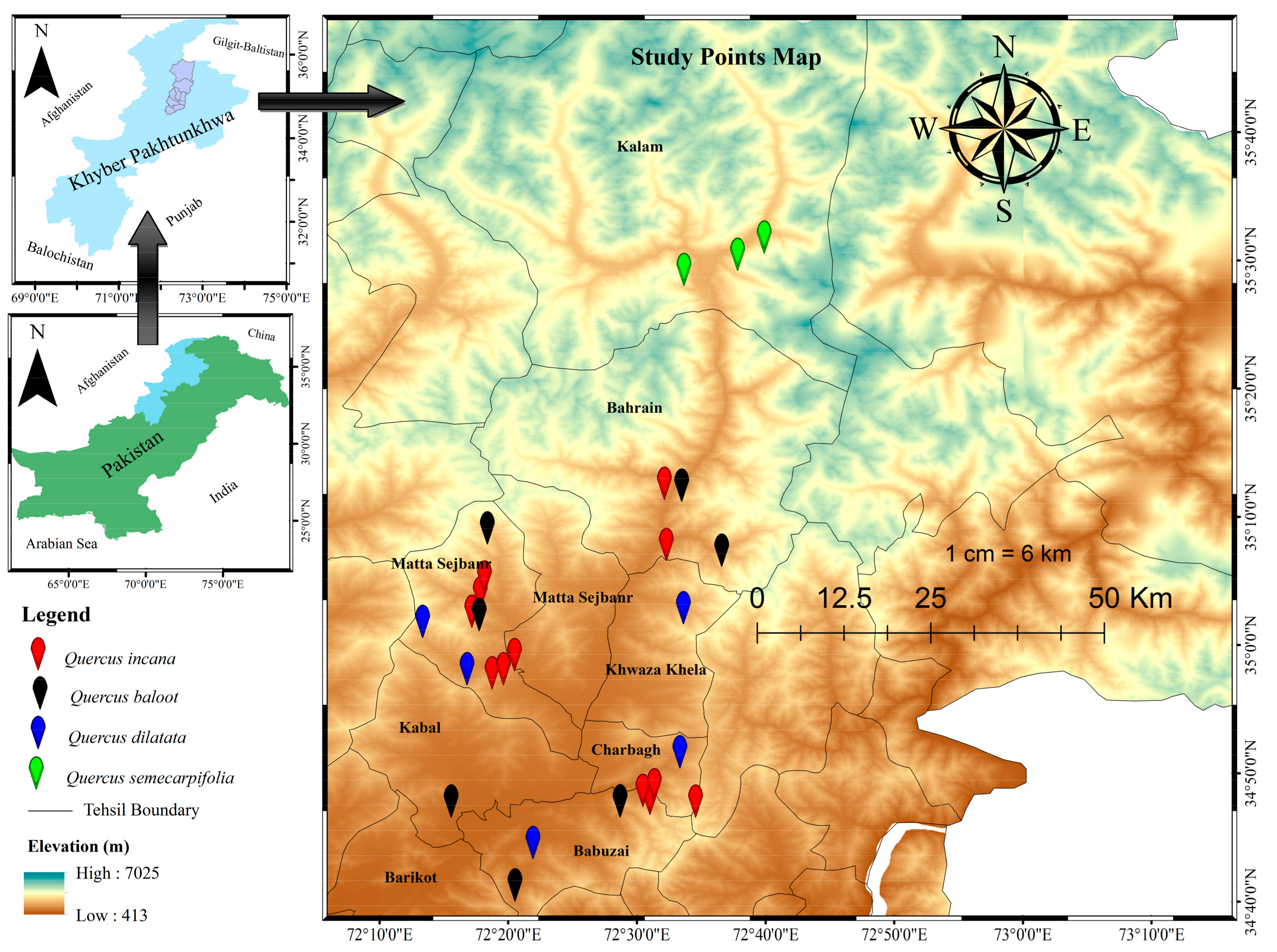
The 30 sampled oak forest stands of different species revealed the dominance of Q. incana (mean IVI = 84 ± 1.2) with the lowest cumulative variance percentage (

Table 1. Stand structure attributes for trees, seedlings, and saplings of four Oak species sampled and their pair wise comparisons.

Parameter	Species Name	Acronym	Min	Max	Mean ± SE	CV%	p-Values
Importance value index	Q. incana	IVI Qi	52	100	84 ± 1.2	20
	Q. dilatata	IVIQd	5	82	40 ± 4.7	83	0.004
	Q. baloot	IVIQb	10	100	76 ± 2.7	41
	Q. semecarpifolia	IVIQs	3	100	62 ± 10	67
Basal Area/stand	Q. incana	BAQi	45	1348	410 ± 27	93
	Q. dilatata	BAQd	29	925	301 ± 44	103	0.025
	Q. baloot	BAQb	111	846	417 ± 52	112
	Q. semecarpifolia	BAQs	104	1172	851 ± 125	59
Tree Density/stand	Q. incana	DQi	44	232	118 ± 4.12	52
	Q. dilatata	DQd	7	149	68 ± 10	88	0.008
	Q. baloot	DQb	27	209	110 ± 6.5	59
	Q. semecarpifolia	DQs	97	160	122 ± 8.3	27
Seedling Density/stand	Q. incana	SQi	32	352	161 ± 7.7	67	<0.001
	Q. dilatata	SQd	59	136	98 ± 8.6	35
	Q. baloot	SQb	3	64	32 ± 3.3	61
	Q. semecarpifolia	SQs	57	207	107 ± 21	80
Sapling Density/stand	Q. incana	SpQi	36	320	142 ± 5.6	55
	Q. dilatata	SpQd	20	124	57 ± 5.1	44	0.03
	Q. baloot	SpQb	16	57	80 ± 5.3	47
	Q. semecarpifolia	SpQs	40	124	91 ± 5.6	37

). The structural characteristics of stand density (232 stems/stand) and basal area (1348/stand) were higher for Q. incana. Likewise, the numbers of seedlings were higher than saplings and trees, indicating good regeneration potential in the oak forest stands. Among the oak species, Q. semecarpifolia attained the highest basal area (1172/4000 m²) and was found to be a fairly regenerating species (Trees density < saplings > seedlings). Conversely, Q. dilatata and Q. baloot showed poor regeneration potential (Tree density > saplings > seedlings). Species richness was 8–12 tree/stand had been found in communities with fourteen associated species, of which P. roxburghii (IV = 10.9 ± 10%) and O. ferruginea (7.8 ± 4.9%) shared higher importance values after oak specie and emerged as the most common co-dominant species forming the second tree stratum (Table 1).

Generally, the oak forest in the area has always been threatened by human intervention, especially the cutting down of trees in the forest canopy. The local inhabitants chopped down almost the entire forest patches in some areas, which led to little or no oak tree populations. The communities of Q. semecarpifolia (30.8 ± 13.0 stem/stand) and Q. incana (29.4 ± 9.4 stem/stand) were mostly affected with the highest number of cut trees. In contrast, the lowest number of cut trees and other anthropogenic disturbances were recorded in Q. baloot and Q. dilatata communities (

Table 2. Density of cut and dead trees due to anthropogenic disturbance.

	Quercus incana	Quercus dilatata	Quercus baloot	Quercus semecarpifolia
Cut	29.48 ± 9.44	12.5 ± 7.5	7.5 ± 3.3	30.83 ± 13.09
Dead	5.62 ± 2.3	0	0	7.5 ± 2.5

).

Furthermore, the pairwise statistical analysis (

Table 3. Compares the structural attributes of four oak species in the forests.

	IVI	Stand Basal Area (m2 ha−1)	Stand Tree Density ha−1	Seedling Density ha−1
Qs-Qd	0.578	0.541	0.520	0.758
Qs-Qb	0.069	0.131	0.081	0.543
Qs-Qi	<0.001	0.004	0.001	<0.001
Qd-Qb	0.206	0.368	0.270	0.764
Qd-Qi	0.006	0.023	0.010	<0.001
Qb-Qi	0.134	0.172	0.145	0.001

) showed significant differences in the structural and dendrometric parameters such as Importance values (p = 0.004), especially between Q. semecarpifolia and Q. incana (p < 0.001) and Q. dilatata and Q. incana (p = 0.006). The four Oak species’ significant difference was recorded among the basal area m²/ha (p = 0.025) and density ha⁻¹ (p = 0.008). However, the density of Q. semecarpifolia and Q. incana (p = 0.001) and between Q. dilatata and Q. incana (p = 0.010) forest stands varied significantly when compared with the basal area of these species. Correspondingly, seedling density among the four oak species exhibited significant variation (p < 0.001) and identical patterns. For instance, the pairwise differences between Q. semecarpifolia and Q. incana (p < 0.001) and Q. dilatata and Q. incana (p < 0.001), and Q. baloot and Q. incana (p = 0.001) were obtained (Table 3).

The height size classes of the Oak species show inverse J-shape distribution (Figure 2). The number of seedlings was lower than saplings in species indicating low regeneration potential. Similarly, the number of individuals in height size classes progressively decreases with an increase in height. The pattern of diameter at breast height (DBH) was the same for Q. semecarpifolia and Q. incana, in which the frequencies decreased with an increase in diameter at breast height. However, the pattern is a little irregular in Q. baloot and Q. dilatata e.g., in Q. dilatata frequencies of 11–20 cm DBH and 51–60 cm DBH were highest while the remaining DBH classes follow progressive decreasing trends in frequencies while in Q. baloot the trend is uniformed except for 51–60 cm dbh where the frequencies increases than the proceeding and preceding DBH size class.

The stems stumped of three Oak species collected have age ranges between 13–42 years. The age structure of stands was dominated by Q. incana 19–25 age group (45%), followed by 25–30 (34%), while the remaining were trees aged between 31–42 years. Similarly, in Q. dilatata, the age group 13–18 years was highest (65%) while the rest ranged from 19–36 years. In Q. baloot dominated stands the age group 19–25 years was frequent (32%) followed by the age group 13–18 years and 25–30 years (25% each) while the rest were having age of 31–36 years. Overall, the age structure represents young communities with lower class classes in most of the stands dominated by Oak species (Figure 3).

There were 18 distinct tree species linked to the four groups of oak-dominated woodland. According to a life table for seedlings, saplings, and tree species, saplings make up most of the population in forests where oak trees predominate (

Table 4. Life table constructed for the four Oak species recorded in 30 forest stands.

	Ax	Ix	Dx	Qx	Lx	Tx	Ex
Seedling	3845	1197.81	−834.58	−0.69	1615.11	667.60	0.56
Sapling	6524	2032.39	152.64	0.075	1956.08	−947.51	−0.47
Very small Trees	6034	1879.75	787.85	0.419	1485.83	−2903.58	−1.55
Small Trees	3505	1091.9	794.70	0.728	694.55	−4389.41	−4.019
Medium Trees	954	297.19	215.26	0.72	189.57	−5083.96	−17.106
Large Tree	263	81.931	57.009	0.69	53.43	−5273.52	−64.36
Giant Tree	80	24.922	24.92	1	12.46	−5326.95	−213.74

Note: Ax (Number of Individuals); Ix (Rate of survival); Dx (the number of deaths); Qx (Stage or age-specific mortality); Lx (periodical longevity); Tx (longevity); Ex (expected longevity).

). While gigantic trees have a short lifespan, saplings, and little trees have a long one. The highest rate of survival (Ix) was revealed by saplings, followed by seedlings, and the lowest rate of survival was found for giant trees, most of which were old and fell for various economic reasons. Compared to other tree plants, extremely few small trees have been found to have a modest survival rate. Stage (age) specific mortality (Qx): Mortality was shown to be lowest for seedlings and very tiny trees due to their limited utility and environmental adaptation and greatest for gigantic trees, followed by medium size trees. Trees of little and medium sizes die out at a moderate pace. The mean expectancy of additional life (Ex) for communities where oak predominates revealed that seedlings reached the highest value of 0.55. Very tiny trees in the community size class had a maximum mean expectancy of life value of −1.54, while saplings displayed −0.46 values (Table 4). All stands showed a −0.213 life expectancy for giant trees. In addition, the individuals’ oak species life tables are presented in Appendix A (

Table A1. Quercus baloot life table community of oak-dominated forests.

	Ax	Ix	Dx	Qx	Lx	Tx	Ex
Very small Trees	936	291.588	−355.452	−1.21902	469.314	667.601	2.28953
Small Trees	2077	647.040	−48.7465	−0.07534	671.413	198.286	0.30645
Medium Trees	2233	695.787	374.752	0.53860	508.416	−473.17	−0.6799
Large Tree	1031	321.034	190.093	0.59212	225.987	−981.5	−3.054
Giant Tree	420	130.940	98.9898	0.75599	81.4457	−1207.5	−9.2213
Very small Trees	103	31.9507	24.1796	0.75677	19.8609	−1288.9	−40.344
Small Trees	25	7.77110	7.77110	1	3.88555	−1308.8	−168.43

Note: Ax (Number of Individuals); Ix (Rate of survival); Dx (the number of deaths); Qx (Stage or age-specific mortality); Lx (periodical longevity); Tx (longevity); Ex (expected longevity).

,

Table A2. Quercus dilatata life table community of oak-dominated forests.

	Ax	Ix	Dx	Qx	Lx	Tx	Ex
Very small Trees	399	124.299	−51.4019	−0.41353	150	667.601	5.37092
Small Trees	564	175.700	−88.0949	−0.50139	219.744	517.601	2.94592
Medium Trees	847	263.795	57.6075	0.21837	234.992	297.852	1.12910
Large Tree	662	206.188	116.925	0.56708	147.725	62.8607	0.30487
Giant Tree	287	89.2626	68.6029	0.76855	54.9612	−84.8647	−0.95073
Very small Trees	66	20.6597	13.0078	0.62962	14.1558	−139.826	−6.76803
Small Trees	25	7.65186	7.65186	1	3.82593	−153.982	−20.1234

Note: Legends are the same as that of Table A1.

,

Table A3. Quercus semecarpefolia life table community of oak-dominated forests.

	Ax	Ix	Dx	Qx	Lx	Tx	Ex
Very small Trees	25	78.8162	−60.7477	−0.77075	109.19	667.601	8.47035
Small Trees	448	139.563	39.4470	0.28264	119.840	558.411	4.00111
Medium Trees	321	100.116	−12.3832	−0.12369	106.308	438.570	4.3805
Large Tree	361	112.5	68.4384	0.60834	78.2807	332.262	2.95344
Giant Tree	141	44.0615	27.2196	0.61776	30.4517	253.981	5.76425
Very small Trees	54	16.8419	10.7476	0.63815	11.4680	223.529	13.2722
Small Trees	20	6.09423	6.09423	1	3.04711	212.061	34.7971

Note: Legends are the same as that of Table A1.

and

Table A4. Quercus incana life table community of oak-dominated forests.

	Ax	Ix	Dx	Qx	Lx	Tx	Ex
Very small Trees	2257	703.115	−366.978	−0.52193	886.604	667.601	0.9494
Small Trees	3435	1070.09	250.181	0.23379	945.002	−219.00	0.2046
Medium Trees	2632	819.911	367.692	0.44845	636.065	−1164.0	1.4196
Large Tree	1452	452.219	419.210	0.92700	242.614	−1800.0	3.9805
Giant Tree	106	33.0088	20.5477	0.62249	22.7349	−2042.69	−61.883
Very small Trees	40	12.4610	9.34579	0.75	7.78816	−2065.42	−165.75
Small Trees	10	3.11526	3.11526	1	1.55763	−2073.21	−665.5

Note: Legends are the same as that of Table A1.

).

Two distinct and obvious gradients in the stand structure were found in RDA-ordination, coupled with a third, weaker gradient, across all the stands. Axis 1 and 2 contributed 32.7% of the variance, whereas the ordination accounted for 41.3% of the variability in stand structure data (

Table 5. Summary statistics of RDA analysis axes correlation and biplot scores of the environmental variables.

Axes				Axis 1	Axis 2	Axis 3
Eigenvalue				3.94	2.61	1.72
Variance in species data
% of variance explained				19.7	13	8.6
Cumulative % explained				19.7	32.7	41.3
Pearson Corr., Response-Pred. *				0.90	0.96	0.71
Kendall Corr., Response-Pred.				0.72	0.70	0.48
Variable	Correlation			Biplot S Scores
	Axis 1	Axis 2	Axis 3	Axis 1	Axis 2	Axis 3
Elevation (m)	0.47 **	−0.51 **	0.22	1.66	−1.47	0.52
Slope (Degrees)	0.25	−0.21	0.33 *	0.89	−0.61	0.78
Clay (%)	0.29	−0.38 *	−0.24	1.04	−1.08	−0.56
Silt (%)	−0.24	0.10	0.37 *	−0.84	0.30	0.87
Sand (%)	0.08	0.08	−0.23	0.28	0.25	−0.53
pH (1:5)	0.20	−0.38 *	−0.23	0.73	−1.09	−0.53
Organic matter (%)	0.28	−0.26	0.24	0.99	−0.74	0.56
Lime (%)	0.21	−0.16	0.031	0.74	−0.47	0.07
Nitrogen (%)	0.01	0.07	0.19	0.057	0.203	0.46
Phosphorus (mg/Kg)	−0.33 *	0.22	0.15	−1.18	0.65	0.37
Potassium (mg/Kg)	−0.24	−0.66 ***	−0.04	−0.85	−1.88	−0.10
Maximum temperature (°C)	0.29	0.06	−0.45 **	1.02	0.19	1.05
Minimum temperature (°C)	0.23	0.12	0.02	0.82	0.34	0.06
Precipitation (mm)	−0.47 **	−0.03 *	0.47 **	−1.65	−0.10	1.10
Relative humidity (%)	−0.77 ***	−0.05	−0.35 *	−2.73	−0.17	−0.82

Note: * (p < 0.05); ** (p < 0.01); *** (p < 0.001).

). The strong gradient on axis 1 was elevation (r = 0.47, p < 0.01), precipitation (r = −0.47, p < 0.01), relative humidity (r = −0.77, p < 0.001), and Phosphorusphosphorus (r = −0.33, p < 0.05). Similarly, on axis 2, the gradient of environmental factors was strongly explained by Potassium (r = −0.66, p < 0.001) and elevation (r = −0.51, p < 0.05). In contrast, axis 3 has a strong gradient of precipitation (r = 0.47, p < 0.01) and maximum temperature (r = 0.45, p < 0.01). Likewise, in biplot scores, the bulk of explainable variables accommodated on axes 1 and 2 (Table 5 and Figure 4).

Axis 1 has the maximum biplot score for relative humidity (2.72), followed by precipitation (−1.65) and elevation (1.66). Similarly, on axis 2, Potassium (−1.88) and elevation (−1.46) revealed the highest biplot scores, respectively. In the two-dimensional biplot, these factors are presented as red arrows indicating their vital role in shaping the stand structure of an Oak-dominated forest.

4. Discussion

The present study describes the tree vegetation composition, age structure, and distribution pattern of oak-dominated forests in Pakistan’s Swat Hindu-Kush ranges. Even though four oak species predominated the vegetation, showing structural and floristic heterogeneity and having a complex relationship with the environment [3]. The three oak communities were found in the research region at a moderate height of 1160 to 2289 m a.s.l. and were dominated by Q. incana, Q. baloot, and Q. dilatata. While the pure population of Q. semecarpifolia was found at high elevations, the species-rich Q. incana community thrived at lower altitudes (1160 m). The areas with medium elevations had most of the Q. baloot and Q. dilatata groups. The oak communities’ co-dominant species were the broad-leaved Olea ferruginea and coniferous Pinus roxburghii. Numerous studies categorizing the northern Pakistani Himalayan, Hindukush, and Karakoram regions have shown a similar communal structure. Pinus roxburghii co-dominate with Q. baloot, Q. dilatata, and Olea ferruginea [30]; these reports were subsequently confirmed by [17,18,19] in Pinus wallachiana populations in the same area. Additionally, they showed how the communities were distributed depending on elevation, which is consistent with the present research results. The current study’s findings on the distribution pattern and occurrences of various species in oak ecosystems are also compatible with [42].

The regeneration status could have been higher due to the number of trees reported in the communities. In stands of oak forests, older trees often start to regenerate after 30 to 40 years, and saplings frequently survive in significant numbers in harsh environments [43]. Most of the stated forest ages in our research region were relatively young, which might indicate inadequate levels of regeneration. It is evident from this research that if forests are adequately maintained, oak will regenerate, especially in good seed years as the forest ages. However, other conditions start to matter after this stage and impact the oak saplings’ survival ability. As shown for oak species in the Hindukush regions in the present research and the same genus [44], this demonstrates that ontogeny significantly influences resource requirements. Competition within the regeneration layer is essential to how well oak regenerates.

Oak seedlings have been observed to be hampered by several trees, shrubs, and plant species [45,46,47]. Since oaks are considered species that need high quantities of light [48], any disruption of the canopy cover in closed forests improves conditions for oak seedlings and saplings. Competing Pinus species and Olea ferruginea regeneration had a role in this situation. Where Pinus species and Olea ferruginea regeneration was abundant, oak regeneration will be lagged, and vice versa. Pinus seedlings naturally outcompete oak saplings because of their exotic nature [49]. When combined with the older age’s saplings, our findings of low oak seedling-to-sapling ratios and greater sapling-to-tree ratios in many stands may indicate that current seedling recruitment rates are likewise low in these ecosystems. If present regeneration rates are abnormally low, it is unclear what is causing the slowing or stopping of regeneration in this case. However, one of the main co-dominant species in the oak woodlands was identified as Pinus roxburghii [50,51,52]. Apart from land conversion [53], conifer encroachment is thought to be the most significant threat to the survival of oak forests; nevertheless, in the oak-dominated stands, this is likely to be the main factor restricting seedling and sapling recruitment [17,30]. As a result, it is known that replacing oak with other species following many forms of disturbance is of recurrent concern [54].

To determine the static life table of the oak-dominated forest population in the various study areas, we calculated the survival number of standardization (Ix), the number of deaths (Dx), longevity (Tx), expected longevity (Ex), and periodic longevity (Lx), for each age class, as shown in Table 3. According to research, Q. baloot saplings have the highest life expectancy of the tree, while Quercus dilatata seedlings are the most prevalent in woods. Due to its economic and commercial purposes, it was discovered that trees in all oak-dominated forests had a poor survival rate. Due to their strong tolerance to cold and drought, saplings were found to have the best survival rates across all communities, whereas large trees had the lowest rates. Conferring to [55], various ecological parameters are crucial for supporting these tree species’ development and survival. Many researchers studying oak forests, such as [56,57,58], observed high death rates for large trees.

Stand structure gradients revealed weakly correlated associations with certain environmental conditions, i.e., lime and nitrogen percentages. The parameters strongly related to the stand structure were climate, elevation, and soil nutrients, which showed the highest correlation across the sampling sites. Negative impacts of precipitation, temperature, relative humidity, altitude, Potassium, and phosphorus content on stand structure are evident. Numerous studies suggested higher temperatures could shorten germination times and decrease seedling richness [59,60]. For instance, [61] reported that increasing temperatures reduced the germination and survival of A. pseudoplatanus and A. platanoides. This trend may be explained by the likelihood that warming would lessen the competitive advantage from which this species previously benefited under the earlier colder environment [62]. Furthermore, since warming increases surface evapotranspiration and decreases soil moisture, creating a water deficit throughout the growing season might hinder recruitment [61,63,64]. For instance, Linares [65] exposed that yew (Taxus baccata) regrowth at its southern boundary was limited by water availability [66,67,68]. In addition, tree mortality brought on by physiological stress and temperature, the depletion of starch pools, and interactions with other climate-mediated processes like insect outbreaks and wildfires may increase due to global warming [69,70,71,72,73].

5. Conclusions

This research is unique because it assessed oak species’ stand structure, regeneration status, population dynamics, and its relation with the environmental variables. The communities had a fair regeneration status showing strong relation with environmental variables, particularly the elevation gradient. This advances our understanding of the community structure of oak-dominated forests across the elevation gradient, and the species in other regions may follow the same distribution pattern. Apart from local factors, i.e., soil and environmental, regional and global climatic factors may also limit the distribution and dynamics of these forests in the future. In addition, the link between site moisture state, stand architecture, and oak recruitment in the Hindu Kush mountain range requires further study. This study better understood the mechanisms driving vegetation distribution in similar or other vegetation types at adjoining high mountain ranges in Pakistan, India, and Afghanistan. The forests were mostly human-conserved. However, reports of chopped and dead trees suggest human interference. As climate change becomes more significant and land managers are forced to account for these changes in their ecosystem management plans, it may be especially vital to understand the linkages between oak regeneration and site environment state. We suggest a more extensive study at the local and regional levels to reveal the interactions between these forests’ vegetation and environment by including several additional biotic and abiotic components into account.

References

1. Champion, S.H.; Seth, S.K.; Khattak, G. Forest Types of Pakistan; Pakistan Forest Institute: Peshawar, Pakistan, 1965. [Google Scholar]
2. Khan, N.; Shaukat, S.S.; Ahmed, M.; Siddiqui, M.F. Vegetation-environment relationships in the forests of Chitral district Hindukush range of Pakistan. J. For. Res. 2013, 24, 205–216. [Google Scholar] [CrossRef]
3. Khan, N.; Ahmed, M.; Wahab, M.; Ajaib, M. Phytosociology, structure and physiochemical analysis of soil in Quercus baloot Griff, Forest District Chitral Pakistan. Pak. J. Bot. 2010, 42, 2429–2441. [Google Scholar]
4. Ren, G.; Deng, B.; Shang, Z.; Hou, Y.; Long, R. Plant communities and soil variations along a successional gradient in an alpine wetland on the Qinghai-Tibetan Plateau. Ecol. Eng. 2013, 61, 110–116. [Google Scholar] [CrossRef]
5. Ahmed, M.; Husain, T.; Sheikh, A.; Hussain, S.S.; Siddiqui, M.F. Phytosociology and structure of Himalayan forests from different climatic zones of Pakistan. Pak. J. Bot. 2006, 38, 361. [Google Scholar]
6. Siddiqui, M.; Moinuddin, A.; Nasrullah, K.; Khan, I. A quantitative description of moist temperate conifer forests of Himalayan region of Pakistan and Azad kashmir. Int. J. Biol. Biotechnol. 2010, 7, 175–185. [Google Scholar]
7. Ahmed, M.; Shaukat, S.S.; Siddiqui, M.F. A multivariate analysis of the vegetation of Cedrus deodara forests in Hindu Kush and Himalayan ranges of Pakistan: Evaluating the structure and dynamics. Turk. J. Bot. 2011, 35, 419–438. [Google Scholar] [CrossRef]
8. Zhang, J.-T.; Zhang, F. Diversity and composition of plant functional groups in mountain forests of the Lishan Nature Reserve, North China. Bot. Stud. 2007, 48, 339–348. [Google Scholar]
9. Shaheen, H.; Khan, S.M.; Harper, D.M.; Ullah, Z.; Qureshi, R.A. Species diversity, community structure, and distribution patterns in western Himalayan alpine pastures of Kashmir, Pakistan. Mt. Res. Dev. 2011, 31, 153–159. [Google Scholar] [CrossRef] [Green Version]
10. Baig, M.B.; Shabbir, S.; Khan, N.; Ahmad, I.; Straquadine, G.S. The history of social forestry in Pakistan: An overview. Int. J. Soc. For. 2008, 1, 167–183. [Google Scholar]
11. Wahab, M. Population Dynamics and Dendrochronological Potential of Pine Tree Species from District Dir. Ph.D. Thesis, Federal Urdu University of Arts, Science And Technology, Karachi, Pakistan, 2011. [Google Scholar]
12. Barbour, M.G.; Burk, J.H.; Pitts, W.D. Terrestrial Plant Ecology; Benjamin Cummings: Menlo Park, CA, USA, 1987. [Google Scholar]
13. Burke, A. Classification and ordination of plant communities of the Naukluft Mountains, Namibia. J. Veg. Sci. 2001, 12, 53–60. [Google Scholar] [CrossRef]
14. Mucina, L. Conspectus of classes of European vegetation. Folia Geobot. 1997, 32, 117–172. [Google Scholar] [CrossRef]
15. Ma, M.; Zhou, X.; Ma, Z.; Du, G. Composition of the soil seed bank and vegetation changes after wetland drying and soil salinization on the Tibetan Plateau. Ecol. Eng. 2012, 44, 18–24. [Google Scholar] [CrossRef]
16. Stewart, R.R. Check list of the plants of Swat State, Northwest Pakistan. Pak. J. Forest. 1967, 17, 457–528. [Google Scholar]
17. Rahman, I.U.; Khan, N.; Ali, K. Classification and ordination of understory vegetation using multivariate techniques in the Pinus wallichiana forests of Swat Valley, northern Pakistan. Sci. Nat. 2017, 104, 144. [Google Scholar] [CrossRef]
18. Siddiqui, M.F.; Arsalan, A.; Ahmed, M.; Hussain, M.I.; Iqbal, J.; Wahab, M. Assessment of understorey vegetation of Malam Jabba Forest, KPK after cleanup operation using multivariate techniques. J. Teknol. 2016, 78, 9–17. [Google Scholar] [CrossRef] [Green Version]
19. Rahman, A.; Khan, N.; Bräuning, A.; Ullah, R.; Rahman, I.U. Effects of environmental and spatial gradients on Quercus-dominated Mountain forest communities in the Hindu-Kush ranges of Pakistan. Saudi J. Biol. Sci. 2022, 29, 2867–2877. [Google Scholar] [CrossRef]
20. Sher, H.; Alyemeni, M.N. Cultivation and domestication study of high value medicinal plant species (its economic potential and linkages with commercialization). Afr. J. Agric. Res. 2010, 5, 2462–2470. [Google Scholar]
21. Qasim, M.; Hubacek, K.; Termansen, M.; Fleskens, L. Modelling land use change across elevation gradients in district Swat, Pakistan. Reg. Environ. Chang. 2013, 13, 567–581. [Google Scholar] [CrossRef]
22. Akhtar, N.; Rashid, A.; Murad, W.; Bergmeier, E. Diversity and use of ethno-medicinal plants in the region of Swat, North Pakistan. J. Ethnobiol. Ethnomed. 2013, 9, 25. [Google Scholar] [CrossRef] [Green Version]
23. Shinwari, Z.; Khan, A.; Nakaike, T.; Kyōkai, N. Medicinal and Other Useful Plants of District Swat, Pakistan; Al-Aziz Communications: Peshawar, Pakistan, 2003; pp. 97–98. [Google Scholar]
24. Zeb, S.A.; Khan, S.M.; Ahmad, Z. Phytogeographic elements and vegetation along the river Panjkora-Classification and ordination studies from the Hindu Kush Mountains range. Bot. Rev. 2021, 87, 518–542. [Google Scholar] [CrossRef]
25. Hussain, F.; Ilahi, I. Ecology and Vegetation of Lesser Himalayas Pakistan; Department of Botany, University of Peshawar: Peshawar, Pakistan, 1991; p. 187. [Google Scholar]
26. Ilyas, M.; Qureshi, R.; Akhtar, N.; Munir, M.; Haq, Z. Vegetation analysis of Kabal valley, district Swat, Pakistan using multivariate approach. Pak. J. Bot. 2015, 47, 77–86. [Google Scholar]
27. Ali, K.; Ahmad, H.; Khan, N.; Jury, S. Future of Abies pindrow in Swat district, northern Pakistan. J. For. Res. 2014, 25, 211–214. [Google Scholar] [CrossRef]
28. Baillie, M.G.; Pilcher, J.R. A simple crossdating program for tree-ring research. Tree-Ring Bull. 1973, 33, 7–14. [Google Scholar]
29. Woch, M.W.; Kapusta, P.; Stefanowicz, A.M. Variation in dry grassland communities along a heavy metals gradient. Ecotoxicology 2016, 25, 80–90. [Google Scholar] [CrossRef] [Green Version]
30. Khan, N.; Ali, K.; Shaukat, S. Phytosociology, structure and dynamics of Pinus roxburghii associations from Northern Pakistan. J. For. Res. 2014, 25, 511–521. [Google Scholar] [CrossRef]
31. Lu, R. Methods of Soil Agricultural Chemical Analysis; China Agricultural Science and Technology Press: Beijing, China, 2000. [Google Scholar]
32. Bray, R.H.; Kurtz, L.T. Determination of total, organic, and available forms of Phosphorusphosphorus in soils. Soil Sci. 1945, 59, 39–46. [Google Scholar] [CrossRef]
33. Mueller-Dombois, D.; Ellenberg, H. Aims and Methods of Vegetation Ecology; Wiley: New York, NY, USA, 1974. [Google Scholar]
34. Cottam, G.; Curtis, J.T. The use of distance measures in phytosociological sampling. Ecology 1956, 37, 451–460. [Google Scholar] [CrossRef]
35. Saeed, S.; Jaleel, W.; Naqqash, M.N.; Saeed, Q.; Zaka, S.M.; Sarwar, Z.M.; Ishtiaq, M.; Qayyum, M.A.; Sial, M.U.; Batool, M. Fitness parameters of Plutella xylostella (L.) (Lepidoptera; Plutellidae) at four constant temperatures by using age-stage, two-sex life tables. Saudi J. Biol. Sci. 2019, 26, 1661–1667. [Google Scholar] [CrossRef]
36. Ali, S.; Li, S.; Jaleel, W.; Musa Khan, M.; Wang, J.; Zhou, X. Using a two-sex life table tool to calculate the fitness of Orius strigicollis as a predator of Pectinophora gossypiella. Insects 2020, 11, 275. [Google Scholar] [CrossRef]
37. Khan, M.; Khan, S.M.; Ilyas, M.; Alqarawi, A.A.; Ahmad, Z.; Abd_Allah, E.F. Plant species and communities assessment in interaction with edaphic and topographic factors; an ecological study of the mount Eelum District Swat, Pakistan. Saudi J. Biol. Sci. 2017, 24, 778–786. [Google Scholar] [CrossRef]
38. Jongman, E.; Jongman, S.R.R. Data Analysis in Community and Landscape Ecology; Cambridge University Press: Cambridge, UK, 1995. [Google Scholar]
39. Ter Braak, C.J. The analysis of vegetation-environment relationships by canonical correspondence analysis. Vegetatio 1987, 69, 69–77. [Google Scholar] [CrossRef]
40. Lepš, J.; Šmilauer, P. Multivariate Analysis of Ecological Data Using CANOCO; Cambridge University Press: Cambridge, UK, 2003. [Google Scholar]
41. Zuur, A.F.; Ieno, E.N.; Smith, G.M. Analysing Ecological Data; Springer: New York, NY, USA, 2007; Volume 680. [Google Scholar]
42. Ali, F.; Khan, N.; Ahmad, A.; Khan, A.A. Structure and biomass carbon of Olea ferruginea forests in the foot hills of Malakand division, Hindukush range mountains of Pakistan. Acta Ecol. Sin. 2019, 39, 261–266. [Google Scholar] [CrossRef]
43. Annighöfer, P.; Beckschäfer, P.; Vor, T.; Ammer, C. Regeneration patterns of European oak species (Quercus petraea (Matt.) Liebl., Quercus robur L.) in dependence of environment and neighborhood. PLoS ONE 2015, 10, e0134935. [Google Scholar] [CrossRef]
44. Abdala-Roberts, L.; Galmán, A.; Petry, W.K.; Covelo, F.; De la Fuente, M.; Glauser, G.; Moreira, X. Interspecific variation in leaf functional and defensive traits in oak species and its underlying climatic drivers. PLoS ONE 2018, 13, e0202548. [Google Scholar] [CrossRef]
45. Löf, M. Establishment and growth in seedlings of Fagus sylvatica and Quercus robur: Influence of interference from herbaceous vegetation. Can. J. For. Res. 2000, 30, 855–864. [Google Scholar] [CrossRef]
46. Löf, M.; Isacsson, G.; Rydberg, D.; Welander, T.N. Herbivory by the pine weevil (Hylobius abietis L.) and short-snouted weevils (Strophosoma melanogrammum Forst. and Otiorhynchus scaber L.) during the conversion of a wind-thrown Norway spruce forest into a mixed-species plantation. For. Ecol. Manag. 2004, 190, 281–290. [Google Scholar] [CrossRef]
47. Alalouni, U.; Brandl, R.; Auge, H.; Schädler, M. Does insect herbivory on oak depend on the diversity of tree stands? Basic Appl. Ecol. 2014, 15, 685–692. [Google Scholar] [CrossRef]
48. Aas, G.; Roloff, A.; Weisgerber, H.; Lang, U.; Stimm, B.; Schütt, P. Quercus petraea (Mattuschka) Lieblein, 1784. Traubeneiche. In Enzyklopädie der Holzgewächse. Handbuch und Atlas der Dendrologie; Wiley-VCH: Weinheim, Gremany, 2002; pp. 1–16. [Google Scholar]
49. Ligot, G.; Balandier, P.; Fayolle, A.; Lejeune, P.; Claessens, H. Height competition between Quercus petraea and Fagus sylvatica natural regeneration in mixed and uneven-aged stands. For. Ecol. Manag. 2013, 304, 391–398. [Google Scholar] [CrossRef]
50. Reed, L.J.; Sugihara, N.G. Northern oak woodlands: Ecosystem in jeopardy or is it already too late? USDA For. Serv. Gen. Tech. Rep. PSW-United States Pac. Southwest For. Range Exp. Stn. (USA) 1987, 100, 59–63. [Google Scholar]
51. Gedalof, Z.e.; Pellatt, M.; Smith, D.J. From prairie to forest: Three centuries of environmental change at Rocky Point, Vancouver Island, British Columbia. Northwest Sci. 2006, 80, 34–46. [Google Scholar]
52. Devine, W.D.; Harrington, C.A. Changes in Oregon white oak (Quercus garryana Dougl. ex Hook.) following release from overtopping conifers. Trees 2006, 20, 747–756. [Google Scholar] [CrossRef]
53. Fuchs, M.A. Towards a Recovery Strategy for Garry Oak and Associated Ecosystems in Canada: Ecological Assessment and Literature Review; Environment Canada, Pacific and Yukon Region: Victoria, BC, Canada, 2001. [Google Scholar]
54. Lorimer, C.G.; Chapman, J.W.; Lambert, W.D. Tall understorey vegetation as a factor in the poor development of oak seedlings beneath mature stands. J. Ecol. 1994, 82, 227–237. [Google Scholar] [CrossRef]
55. Zhang, J.; Hao, Z.; Sun, I.-F.; Song, B.; Ye, J.; Li, B.; Wang, X. Density dependence on tree survival in an old-growth temperate forest in northeastern China. Ann. For. Sci. 2009, 66, 204. [Google Scholar] [CrossRef] [Green Version]
56. Shifley, S.; Smith, W. Diameter Growth, Survival, and Volume Estimates for Missouri Trees [Forest Mensuration]; USDA Forest Service Research Note NC-US North Central Forest Experiment Station (USA). no. 292; North Central Forest Experiment Station: St. Paul, MN, USA, 1982. [Google Scholar]
57. Hicks, R.R. Ecology and Management of Central Hardwood Forests; John Wiley & Sons: New York, NY, USA, 1998. [Google Scholar]
58. Makineci, E. Long term effects of thinning on soil and forest floor in a sessile oak (Quercus petraea (Matlusch) Lieb.) forest in Turkey. J. Environ. Biol 2005, 26, 257–263. [Google Scholar]
59. Lloret, F.; Penuelas, J.; Estiarte, M. Experimental evidence of reduced diversity of seedlings due to climate modification in a Mediterranean-type community. Glob. Chang. Biol. 2004, 10, 248–258. [Google Scholar] [CrossRef]
60. Matías, L.; Jump, A.S. Impacts of predicted climate change on recruitment at the geographical limits of Scots pine. J. Exp. Bot. 2014, 65, 299–310. [Google Scholar] [CrossRef] [Green Version]
61. Carón, M.; De Frenne, P.; Brunet, J.; Chabrerie, O.; Cousins, S.A.; De Backer, L.; Decocq, G.; Diekmann, M.; Heinken, T.; Kolb, A. Interacting effects of warming and drought on regeneration and early growth of Acer pseudoplatanus and A. platanoides. Plant Biol. 2015, 17, 52–62. [Google Scholar] [CrossRef]
62. Qi, J.; Huete, A.; Moran, M.; Chehbouni, A.; Jackson, R. Interpretation of vegetation indices derived from multi-temporal SPOT images. Remote Sens. Environ. 1993, 44, 89–101. [Google Scholar] [CrossRef]
63. Cavender-Bares, J.; Bazzaz, F. Changes in drought response strategies with ontogeny in Quercus rubra: Implications for scaling from seedlings to mature trees. Oecologia 2000, 124, 8–18. [Google Scholar] [CrossRef]
64. Matías, L.; Jump, A.S. Interactions between growth, demography and biotic interactions in determining species range limits in a warming world: The case of Pinus sylvestris. For. Ecol. Manag. 2012, 282, 10–22. [Google Scholar] [CrossRef]
65. Linares, J.C. Shifting limiting factors for population dynamics and conservation status of the endangered English yew (Taxus baccata L., Taxaceae). For. Ecol. Manag. 2013, 291, 119–127. [Google Scholar] [CrossRef]
66. Morin, X.; Augspurger, C.; Chuine, I. Process-Based Modeling of Species’distributions: What Limits Temperate Tree Species’range Boundaries? Ecology 2007, 88, 2280–2291. [Google Scholar] [CrossRef] [Green Version]
67. Jump, A.S.; Mátyás, C.; Peñuelas, J. The altitude-for-latitude disparity in the range retractions of woody species. Trends Ecol. Evol. 2009, 24, 694–701. [Google Scholar] [CrossRef] [Green Version]
68. Peñuelas, J.; Sardans, J.; Estiarte, M.; Ogaya, R.; Carnicer, J.; Coll, M.; Barbeta, A.; Rivas-Ubach, A.; Llusià, J.; Garbulsky, M. Evidence of current impact of climate change on life: A walk from genes to the biosphere. Glob. Chang. Biol. 2013, 19, 2303–2338. [Google Scholar] [CrossRef]
69. Van Mantgem, P.J.; Stephenson, N.L. Apparent climatically induced increase of tree mortality rates in a temperate forest. Ecol. Lett. 2007, 10, 909–916. [Google Scholar] [CrossRef]
70. Allen, C.D.; Macalady, A.K.; Chenchouni, H.; Bachelet, D.; McDowell, N.; Vennetier, M.; Kitzberger, T.; Rigling, A.; Breshears, D.D.; Hogg, E.T. A global overview of drought and heat-induced tree mortality reveals emerging climate change risks for forests. For. Ecol. Manag. 2010, 259, 660–684. [Google Scholar] [CrossRef] [Green Version]
71. McDowell, N.G.; Sevanto, S. The mechanisms of carbon starvation: How, when, or does it even occur at all? New Phytol. 2010, 186, 264–266. [Google Scholar] [CrossRef]
72. Vanderwel, M.C.; Lyutsarev, V.S.; Purves, D.W. Climate-related variation in mortality and recruitment determine regional forest-type distributions. Glob. Ecol. Biogeogr. 2013, 22, 1192–1203. [Google Scholar] [CrossRef]
73. Vilà-Cabrera, A.; Martínez-Vilalta, J.; Galiano, L.; Retana, J. Patterns of forest decline and regeneration across Scots pine populations. Ecosystems 2013, 16, 323–335. [Google Scholar] [CrossRef]
Figure 1. Map of the study area indicating the sampling sites for field study.
Sustainability 15 04002 g001
Figure 2. Height size classes and diameter at breast height of Oak species.
Sustainability 15 04002 g002
Figure 3. Different age classes of the Oak species.
Sustainability 15 04002 g003
Figure 4. Canonical correspondence analysis biplot of the oak stand structural attributes and related environmental variables. Note: Red color arrows indicate environmental factors that have a significant effect on the communities; Blue arrow represents the specie lines; the triangle indicates the sampling sites; Elev (Elevation); R.H. (Relative Humidity); K (Potassium); P (Phosphorus); Precip (Precipitation); Species acronyms are the same as that in Table 1.
Sustainability 15 04002 g004