A Demand-Side Inoperability Input–Output Model for Strategic Risk Management: Insight from the COVID-19 Outbreak in Shanghai, China

Abstract

This paper proposes the dynamic inoperability input–output model (DIIM) to analyze the economic impact of COVID-19 in Shanghai in the first quarter of 2022. Based on the input–output model, the DIIM model introduces the sector elasticity coefficient, assesses the economic loss of the system and the influence of disturbances on other sectors through sectoral dependence, and simulates the inoperability and economic loss changes through time series. A multi-evaluation examination of the results reveals that the degree of inoperability of sub-sectors is inconsistent with the ranking of economic losses and that it is hard to quantify the impact of each sector directly. Different from the traditional DIIM model that only considers the negative part of the disaster, the innovation of this paper is that the negative value of the inoperability degree is used to measure the indirect positive growth of sectors under the impact of the Shanghai pandemic shock. At the same time, policymakers need to consider multi-objective optimization when making risk management decisions. This study uses surrogate worth trade-off to construct a multi-objective risk management framework to expand the DIIM model to enable policymakers to quantify the trade-off between economic benefit and investment costs when making risk management decisions.

1. Introduction

Since the year 2022, the coronavirus disease 2019 (COVID-19) has spread rapidly around the world. As an important port city in China, Shanghai has always faced huge pressure to stem the spread of the virus within Shanghai and beyond. In Shanghai, the number of infected people has climbed by more than 1000 every day since 23 March 2022, and the number of confirmed cases has continued to rise. In accordance with the issues that have developed throughout the process, Shanghai’s preventative and control policies have also been regularly modified. In the first half of 2022, Shanghai’s gross domestic product (GDP) decreased by 5.7% because of the consequences of the COVID-19 pandemic [1]. Starting in March, COVID-19 has spread rapidly in Shanghai, and the production and consumption of various districts in Shanghai have been quickly blocked by the pandemic. The negative economic impact has continuously transmitted feedback through the upstream and downstream industrial chains, which has had a tremendous impact on economic and social production activities. In order to prevent the rapid spread of the pandemic, many districts in Shanghai have adopted lockdown policies since the end of March, as well as static management throughout the city in April and May. During the management period, the national revenue fell precipitously, and the uncertainty caused by the pandemic led to a reduction in national spending, which was then communicated to numerous industry chains via the “bullwhip effect”. From the standpoint of the supply side, the pandemic’s spread has mostly resulted in the suspension of work and reduction in output in a variety of industries, the forced exodus of laborers from the market, the stoppage of production and activities in the internal industrial chain, and the decrease in the availability of intermediate items in the region. In order to successfully deal with the potentially grave impact of COVID-19 on Shanghai, the lockdown policy was lifted, and the strong interdepartmental economic resilience resulted in a dramatic improvement in Shanghai’s key economic indicators after June. The sustainability of the industrial chain has emerged as a crucial central concern in the context of being severely affected by the pandemic. What degree of effect would this industry’s own effects and the spillover effects of linked industries have in this situation? What is the cumulative economic loss suffered by each sector? How can the government optimize cost and benefit when implementing a risk management policy? The present responses to the aforementioned issues have significant policy implications and practical impacts.

2. Literature Review

Research methodologies on the economic impact of disasters fall mostly into three categories: dynamic stochastic general equilibrium models, computable general equilibrium models, and Leontief input–output models. There is a significant amount of research papers on these three techniques, but still have room for advancement: First, there are few literature studies on quantifying and predicting the impact of the pandemic on the economy, especially considering the cascading effect of industries. Second, the perspective of quantitative research needs to be refined and supplemented. At the same time, the existing literature pays little attention to the phased characteristics of the pandemic’s impact on the economy, and it is difficult to give full play to the effect of the introduction and application of the national defense policy after the pandemic. In view of this, this paper uses the Leontief input–output model to measure the final economic loss from the perspective of industrial correlation and pay attention to the staged impact of the pandemic. The Leontief input–output model reflects the quantitative dependence of input and output among various departments in the regional economic system in a balanced state and uses the general equilibrium model of input and output to estimate the departmental indirect economic losses caused by disasters. From the perspective of general static input and output, academic papers evaluate the impact of crisis events on the regional economy from the perspective of industrial association, including two aspects: direct economic loss and indirect economic loss. In this paper, indirect economic loss is defined as the decline in total production caused by the loss effect spreading through the industrial association after the industrial sector is destroyed by the crisis. This loss from the interconnectedness that exists between sectors within the economic system causes a multiplier effect throughout the entire economic system when the immediate disruption of a crisis to an economic sector results in a shortage of attacks or a drop in demand for that sector or a propagation effect. The assessment of indirect economic loss method was first introduced by Cochrance [2], and then widely used [3,4]. There are two shortcomings in the evaluation based on the classical I-O table in the existing literature: First, the disaster evaluation using the input–output method is mostly static analysis, without considering the change of production capacity. Second, the general static input–output model does not consider the elasticity of the economic system. This situation is only true when analyzing long-term time scales, and it is difficult to measure shorter monthly time scales such as this one. Moreover, it is difficult for the classical I-O table to reflect the characteristics of dynamic spatiotemporal changes, especially in the short term after a disaster, such lack of consideration of the elasticity of the economic system makes the loss assessment results in an underestimation.

To solve such problems, based on the I-O model, Hamies [5] proposed the IIM model to analyze the interdependence among various economic sectors and the indirect chain reaction of various sectors under the impact of disasters. In the IIM model, inoperability is used to describe the degree of failure that the economy is affected, and cumulative economic loss is used to measure the overall risk of suffering. However, the IIM model can only be analyzed statically, and there is still room for improvement. Lian and Hamies [3] extended the IIM to a DIIM, which analyzed the time path of sectoral disturbances from catastrophic events to a new economic equilibrium based on the input–output table. Incorporating sectoral linkages, the ability to meet production levels and the demand and supply side impacts of disturbances are estimated. At the same time, DIIM combines the resilience parameter to simulate the departmental recovery path, further expanding the system modeling capabilities of the input–output model and using the ensuing model results to aid policymakers in risk management decisions. Given the initial functionality loss and recovery time of infrastructure before significant public health and natural disasters, DIIM is frequently used to assess the resilience of economic sectors [6,7,8,9]. Policy insights from the DIIM result help to improve disaster resilience planning for future disasters. Huang et al. [10] used the DIIM model to measure the sensitivity and economic loss of 42 sectors in China under COVID-19 impact, as well as to analyze the phased characteristics of the pandemic. Such a method provides additional perspectives for quantifying the impact of the pandemic and supplements detailed data on economic losses across various industries. Depending on the severity of the economic effects, when responding to such severe health public events, the key economic sectors will be prioritized, aiding a speedy recovery. EI Haimer et al. [11] used the improved DIIM model to analyze the impact of the HIN1 influenza virus on the economic system. At the same time, Santos [12] conducted a study based on the workforce absenteeism perspective to assess the sector-by-sector impact under COVID-19 with the DIIM model and simulate potential impacts of "flattening the curve" to contain or mitigate workforce continuity. While there are also some literature studies starting from the supply side, based on the Ghosh model, considering value-added perturbation [13]. The essence of the demand-side model is a quantity model, while the input of the added value of the supply side makes it essentially a price model. Leung et al. [14] introduced the SDIIM model and Xu et al. [15] took the severe snow disaster in South China in 2008 as the research object, based on the SDIIM model and took the disturbance in the added value as input, and showed that from the initial disturbance to the final equilibrium of the net added value, the cost price was between changes in each period. Similarly, Lanndon et al. [16] proposed from the supply side the factors that can quantify the disturbance of the manufacturing system, that is, the system caused by the increase in value-added input, price increase, and production cost increase because of the degradation of the supply chain caused by natural disasters. Although a few existing papers are based on supply-side analysis, and the COVID-19 problem often occurs on the supply side, the demand-side DIIM model is modeled as a forced demand reduction, which is transmitted to other sectors through backwards linkage. As demonstrated by Oosterhaven, supply-side DIIM has more problems than demand-side DIIM [17]. This paper still adopts the demand-side DIIM model, taking into account that the pandemic also has a certain impact on demand-side factors such as residents’ consumption. Moreover, the outbreak of the Shanghai pandemic has been one and a half years since the first half of 2020, when the pandemic was most severe. China’s pandemic prevention policies have allowed many departments to resume work and production to a certain extent. However, the suppression of the demand side and the consumption side by the pandemic in China has not been effectively resolved, and the market lacks vitality. Therefore, it is more necessary to look at the impact of the impact from the demand side. DIIM can identify the path of inoperability for each sector and the overall economic loss in the event of a disaster; meanwhile, risk management can strengthen economic resilience and reduce shock-related losses. For instance, policy prevention and control measures help minimize the rate of inoperability or accelerate recovery time under risk. Hence, policymakers can utilize the analogy of pertinent historical events to develop candidate risk management solutions and assess the efficacy of management after implementation, so as to establish an acceptable balance between numerous cost, benefit, and risk objectives. The surrogate worth trade-off (SWT) is a method in which non-commensurate multi-objective optimization will be explained through a simplified example of commensurate multi-objective optimization. It applies optimization theory to assess the relative worth of further non-commensurable objective increments at a specific value for each objective function. Given the current set of objective levels, it is much clearer for decision-makers to evaluate the relative value of trade-offs rather than the absolute value, determining whether an additional quantity of one objective is more valuable than the other [18]. To analyze each risk management alternative based on the trade-off between investment costs (in monetary units) and benefits (in terms of economic losses recovered), SWT is a suitable method to make decisions. Using recovered economic losses as a measure of benefits illustrates the effect of reducing inoperability and recovery time on reducing economic losses.

In summary, this paper uses the demand-side DIIM model proposed by Lian and Hamies [19] to measure the cascading economic effect resulting from the time-varying workforce unavailability and uses SWT to solve the problem such as what are the tradeoffs in terms of costs, benefits, and risks? What are the impacts of current decisions on future options? The overall components are listed as follows: The first section of this paper constructs a demand-side DIIM model and risk management trade-off method. The second section employs the DIIM model to examine the time-varying path of inoperability degree and the cumulative economic loss in Shanghai during the first half of 2022 under the background of COVID-19. Then, it utilizes the SWT approach for multi-objective risk management to undertake a trade-off analysis. Finally is the summary and conclusion

3. Theoretical Model and Data

3.1. Leontief Input–Output Table and Dynamic Inoperability Input–Output Model (DIIM)

The basic formulation of classic Leontief I-O is given by Equation (1), where x symbolizes the total production output. $a_{ij}$, the Leontief coefficient, indicated the ratio of the input from industry i to industry j, with respect to the total production requirement of industry j. Given n industries, $a_{ij}$ may illustrate the contribution of each industry $i=1,2,3,\dots n$ to the total inputs required by industry j. $c_i$ represents the final demand of the industry, which is defined as the proportion of the industry’s total output destined for final consumption [20].

$$x=A^{*}x+c^{*}⟺\left\{x_i=\sum a_{ij}{x}_i+c_i\right\}\forall I$$

(1)

Based on the classical Leontief I-O table, Santos (2004) [21] proposed the IIM model based on the interconnected systems to quantify the reduction in each sector output when subjected to the initial demand-side negative internal failure or external shocks. Inoperability, defined as the percentage reduction from the ideal output, which is triggered by demand reduction, is the basic risk metric. The details of demand reduction model derivation and an extensive discussion of model components are defined as follows:

$${diag\left(\widehat{x}\right)}^{-1}diag\left(\widehat{x}-\stackrel{\sim }{x}\right)q=A^{*}q+c^{*}$$

(2)

$c^{*}$ is a demand-side perturbation vector expressed in terms of normalized degraded final demand. $A^{*}$ is the interdependency matrix that indicates the degree of coupling of industry sectors. q is the interoperability vector expressed in terms of normalized economic loss. Then, the normalized production loss can be explained as follows [22]:

$$\begin{array}{cc}\hfill NormalizedProductionLoss& =\frac{`\mathit{As}-{\mathit{planned}}^{\prime }ProductionOutput-DegradedProductionOutput}{NominalProduction}\hfill \\ & ={diag\left(\widehat{x}\right)}^{-1}\left(\widehat{x}-\stackrel{\sim }{x}\right)\hfill \end{array}$$

(3)

$diag\left(\widehat{x}\right)$ is the diagonal matrix of the given production output $\widehat{x}$.

Denoting $c^{*}$ as the final demand perturbation to the sector due to the initial shock which can be described as the difference between ‘as-planned’ final demand $\left(\widehat{c}\right)$ and reduced level of final demand $\left(\tilde{c}\right)$, normalized according to the ‘as-planned’ production output $\left(\widehat{x}\right)$. Moreover, the demand-side interdependency matrix $A^{*}$ is related to the original Leontief technical coefficient matrix A, a scalar representation of the elements $A^{*}$ is derived as follow [13,23,24,25]:

$$c^{*}={diag\left(\widehat{x}\right)}^{-1}diag\left(\widehat{c}-\stackrel{\sim }{c}\right)$$

(4)

$$A^{*}={diag\left(\widehat{x}\right)}^{-1}Adiag\left(\widehat{x}\right)$$

(5)

3.1.1. Dynamic Input–Output Model

It should be noted that the above-mentioned concepts and numerical definition in the demand-reduction static IIM model are also applicable to the DIIM model, which only extend additional dynamic and stochastic components [26,27]. Then, to establish DIIM model, the fundamental concepts and mathematical elaboration of conventional dynamic input–output models are used as an example. The basic dynamic I-O model expression is:

$$x\left(t\right)=Ax\left(t\right)+c\left(t\right)+B·x\left(t\right)$$

(6)

The numerical interpretation and notation meaning in Equation (1) regarding also applicable to this formula. The element B is introduced in the dynamic model as the capital coefficient matrix, which measures the willingness of the economy to invest in capital resources (such as machines, land, structures, etc.) [28,29]. When equilibrium is reached in the dynamic model, where $x\left(t\right)=0$, Equation (6) has the same format as Equation (1).

Consider a case where $B=-I$ in Equation (6), as represented in Equation (7), which is utilized to reflect variations in aggregate output caused by demand-supply discrepancies.

$$\dot{x}\left(t\right)=Ax\left(t\right)+c\left(t\right)-x\left(t\right)$$

(7)

Performing derivation to the equation and adding the resilience factor of each sector ($k_1$,$k_2$), as shown in Equation (8), the left-hand side represents the production output adjustment of each sector, the right-hand side reflects the imbalance between the short-term supply and demand side, and $k_i$ represents the production adjustment rate [30].

$$\begin{array}{c}\hfill \left\{\begin{array}{c}d{x}_1\left(t\right)={\left(a_{11}x\right.}_1\left(t\right)+{a_{12}x}_2\left(t\right)+\dots +{a_{1n}x}_n\left(t\right)+c_1\left(t\right)-x_1\left(t\right))k_{1}dt,\\ d{x}_2\left(t\right)={\left(a_{21}x\right.}_1\left(t\right)+{a_{22}x}_2\left(t\right)+\dots +{a_{2n}x}_n\left(t\right)+c_2\left(t\right)-x_2\left(t\right))k_{2}dt\end{array}\right.\end{array}$$

(8)

Because of the multiplicity affecting elements, when the model experiences short-term disturbances, it will be affected not only by the components of the scenario examined in this research paper but also by other various factors [31]. Therefore, to assure the model’s plausibility, a stochastic component is added to the basic dynamic model. The extension IIM formulation is introduced in the following:

$$\frac{dx\left(t\right)}{Ax\left(t\right)+c\left(t\right)-x\left(t\right)}=Kdt+\sigma dz$$

(9)

$$dz=\epsilon \left(t\right)\sqrt{dt}$$

(10)

$$K=Diag\left(k_1,k_2\dots ,k_n\right)$$

(11)

$$\sigma =Diag\left({\sigma }_1,{\sigma }_2,\dots ,{\sigma }_n\right)$$

(12)

$Ax\left(t\right)+c\left(t\right)-x\left(t\right)$ is the interdependency among the sectors of the economy, which is analogous to the classic I-O model. $Kdt$ is the resilience of the economy for its demand and supply to be at the same level in the long term. $\sigma dz$ is the short-term randomness of the dynamic process. $dz=\epsilon \left(t\right)\sqrt{dt}$ is the Wiener process which represents the “random walk “of variables. The notation K is the matrix of the previous production adjustment rate, representing the resilience of each sector. Here, we refer to a formal meaning to it, industry resilience coefficients. The larger the K value, the faster the economic system responds to an imbalance in supply and demand. The $\sigma$(industry resilience deviation matrix) measures the uncertainty of the dynamic process and deviations of the industry resilience coefficient matrix K, implying the uncertainties of the economic sector during the DIIM process. Therefore, a higher $\sigma$ value means a harder prediction of the dynamic path of its behavior. Setting $B=K^{-1}$, then the dynamic I-O table in Equation (6) is equivalent to the DIIM in Equation (8); however, in the DIIM model, B does not represent long-run economic growth. Rather, it denotes short-term resiliencies of the industry sector following disruptive events such as natural hazards or COVID-19 attacks. Since the resiliency of a sector is affected by risk management and public policies, the matrix B can be viewed as a risk management investment coefficient matrix, representing the willingness to invest in risk management for economic sector disasters.

3.1.2. Applying Dynamic Input–Output Model to Establish DIIM

Based on the dynamic input-output model, in this section, the paper establishes the DIIM model.

$$\left\{\begin{array}{c}A\widehat{x}\left(t\right)+\widehat{c}\left(t\right)-\widehat{x}\left(t\right)=0\\ \frac{d\stackrel{\sim }{x}\left(t\right)}{A\stackrel{\sim }{x}\left(t\right)+\stackrel{\sim }{c}\left(t\right)-\stackrel{\sim }{x}\left(t\right)}=Kdt+\sigma dz\end{array}⟹\frac{d\left(\widehat{x}-\stackrel{\sim }{x}\left(t\right)\right)}{A\left(\widehat{x}-\stackrel{\sim }{x}\left(t\right)\right)+\left(\widehat{c}-\stackrel{\sim }{c}\left(t\right)\right)-\left(\widehat{x}+\stackrel{\sim }{x}\left(t\right)\right)}=Kdt+\sigma dz\right.$$

(13)

From the definition $q\left(t\right)$ above in Equation (2), then Equation (13) can be transformed into

$$\frac{dq\left(t\right)}{A^{*}q\left(t\right)+c^{*}\left(t\right)-q\left(t\right)}=Kdt+\sigma dz$$

(14)

The stochastic nature of DIIM represents variables that influence the model fluctuation. This paper only focuses the dynamic aspect of IIM and disregard this sector ($\sigma =0$), then the equation is reduced to the following format [19]:

$$\dot{q}\left(t\right)=K\left[A^{*}q\left(t\right)+c^{*}\left(t\right)-q\left(t\right)\right]$$

(15)

Equation (15) is a standard form of linear first-order differential equations the solution to it is as follows, given the initial condition $q\left(0\right)$:

$$q\left(t\right)=e^{-K\left(I-A^{*}\right)t}q\left(0\right)+\underset{0}{\overset{t}{\int }}{Ke}^{-K\left(I-A^{*}\right)\left(t-z\right)}{c}^{*}\left(z\right)dz$$

(16)

If the final demand $c^{*}\left(t\right)$ is stationary, and then can be further simplified as follows [32]:

$${q\left(t\right)=\left(I-A^{*}\right)}^{-1}{c}^{*}+e^{-K(I-A^{*})t}\left[q\left(0\right)-{\left(I-A^{*}\right)}^{-1}{c}^{*}\right]$$

(17)

3.2. Dynamic Inoperability Input–Output Model

3.2.1. Background

Extending the supply and demand sides of the Leontief matrix, the DIIM model is able to capture the influence that each sector had after the disruption as well as the dynamic process of recovery [33]. Demand-side disturbance is the difference between a scoter’s business-as-usual level of production and the level of production caused by a demand decrease because of a disaster occurrence. It has an impact on production. DIIM is also applicable to each sector’s recovery process. As operational issues lessen alongside the decrease in inoperability level, the department’s final output will gradually rise until it reaches equilibrium.

3.2.2. Demand-Side Perturbation Model

The IIM model can be used to describe the static disturbance on the demand side by calculating the decrease in the final production of goods in the various economic sectors affected by the disaster. This process can also be dynamically displayed by DIIM so that decision-makers can observe how they change and reach an equilibrium level. The dynamic demand-reduction inoperability model can be described as the following, which can be obtained from the row–column relationship of the original Leontief inverse matrix, the demand-side total production output $Ax\left(t\right)+c\left(t\right)$ equals the total supply-side $x\left(t\right)$. However, when there is a perturbation to the demand side in which $c\left(t\right)$ is reduced to a certain value, then the term $Ax\left(t\right)+\widetilde{c\left(t\right)}-x\left(t\right)$ is negative. Therefore, the supply side $x\left(t\right)$ starts to decline until it reaches new equilibrium $\widetilde{x\left(t\right)}$.

The inoperability dynamic process for demand-side reduction can be illustrated as:

$$q\left(t\right)=\left[I-e^{-K\left(I-A^{*}\right)t}\right]{\left(I-A^{*}\right)}^{-1}{c}^{*}$$

(18)

At the initial $q\left(0\right)$, each sector is still in the normal operation stage and has not been affected. Thereafter, the $q\left(t\right)$ will alter dynamically based on the severity of the shock and the risk resilience of the department. Where $K\left(t\right)$ is the industry resilience coefficient used to adjust supply and demand imbalances. The greater K, the more sensitive each sector’s adjustment is to change in final demand. K stands for each department’s risk elasticity, to quantify it more accurately, it is necessary to begin with the department’s overall linkage, and hierarchical holographic modeling (HHM) is a method that is frequently employed to evaluate intricate network interactions [30].

3.2.3. Dynamic Recovery Model

To assess the interdependency recovery rate $K_i$ for sector i, it is assumed that sector i is attacked $(q_i\left(0\right)>0)$ and other sectors are not initially perturbed $(q_j\left(0\right)=0,j\ne i)$.

$$\dot{q}\left(t\right)=K\left[A^{*}q\left(t\right)+c^{*}\left(t\right)-q\left(t\right)\right]$$

(19)

The recovery trajectory for the sector becomes:

$$\dot{q}\left(t\right)=-k_i\left(1-a_{ii}^{*}\right)q_i\left(0\right)$$

(20)

The solution to Equation (20) is:

$$q_i\left(t\right)=e^{-k_i(1-a_{ii}^{*})}{q}_i\left(0\right)=e^{-K(I-A^{*})t}{\left(I-A^{*}\right)}^{-1}{c}^{*}$$

(21)

3.2.4. Sector Recovery and Resilience Analysis

The associated economic losses in the economic system brought about by the crisis disasters have staged characteristics. According to the above analysis, the stage-by-stage nonlinear impact model based on recovery elasticity can be written as follows:

$$q\left(t\right)=\left\{\begin{array}{c}{\left(I-A^{*}\right)}^{-1}{c}^{*}+e^{-K(I-A^{*})t}\left[q\left(0\right)-{\left(I-A^{*}\right)}^{-1}{c}^{*}\right]t_0\le t\le t_I\\ e^{-K(I-A^{*})t}{\left(I-A^{*}\right)}^{-1}{c}^{*}{t}_{I+1}\le t\le t_{II}\end{array}\right.$$

(22)

$A^{*}$ is the interdependency matrix representing the dependency of each sector. K is the resilience coefficient matrix.

If experts take $T_i$ for sector i to recover from its initial inoperability $q_i\left(0\right)>0$ to a $q_i\left(T_i\right)$, the interdependency recovery rate can be assessed as Equation (23), derived from Equation (21) [19]:

$$k_i=\frac{ln\left[q_i\left(0\right)/q_i\left(T_i\right)\right]}{T_i}\left(\frac{1}{1-a_{ii}^{*}}\right)=\frac{w_i}{T_i}={\left(\frac{\lambda }{\tau }\right)}_i\left(\frac{1}{1-a_{ii}^{*}}\right)$$

(23)

Let the symbol $w_i$ denote:

$$\frac{ln\left[q_i\left(0\right)/q_i\left(T_i\right)\right]}{1-a_{ii}^{*}}$$

(24)

$\tau$ is the time when inoperability reduces to some value $q_{\tau }$,the recovery constant is $\lambda$, and collectively the ratio ${(\lambda /\tau )}_i$, representing the term, $\frac{ln\left[q_i\left(0\right)/q_i\left(T_i\right)\right]}{T_i}$ is the recovery-rate parameter. The notation $a_{ii}^{*}$ represents the ith diagonal element in the interdependency matrix $A^{*}$. The smaller the $a_{ii}^{*}$ value, the greater the $(1-a_{ii}^{*})$, indicating the higher degree of dependence for the sector and hence faster recovery, considering interdependency with other sectors. Equation (24) implies that the greater $a_{ii}^{*}$ leads to a greater interdependency recovery rate $k_i$.

To demonstrate the dynamic steps of the above formula, consider the following cases, if the initial inoperability level is defined as 5%, then this will be the value of $q_i\left(0\right)$. Suppose the decision-maker wishes to make the inoperability level 1%, this value will now represent $q_i\left(T_i\right)$. Assume further that experts believe that it would take approximately 10 business days for most professional services sector offices to return to work from an inoperability level of 5% to an inoperability level of 1%, implying a value of $T_i$ of 10 days. Finally, setting 70% of the professional services workforce that is classified as some other workforce in the professional services sector would imply $a_{ii}^{*}$ = 0.7. Applying this would therefore reveal the following uncertain elasticity index $k_i$:

$$k_i=\frac{ln\left[q_i\left(0\right)/q_i\left(T_i\right)\right]}{T_i}\left(\frac{1}{1-a_{ii}^{*}}\right)=\frac{ln(5\%/1\%)}{10(1-0.7)}=0.536$$

(25)

The equation means for the professional service sector, the industry resilience coefficient is 0.536.

3.3. Risk Management Analysis

3.3.1. Cumulative Economic Loss and Net Profit

The economic loss for each sector i can be calculated as the difference between `as-planned’ production output and the degraded production output of the $ith$ sector, which can be rewritten into the function of inoperability of sector i as referred previously.

$$\Delta x_i=x_i-\stackrel{\sim }{x_i}=q_i{x}_i$$

(26)

Moreover, the whole sector economic loss can be summed up as cumulative economic loss $w\left[0\right]$:

$${\Gamma }_{w\left[0\right]}=\sum _{i=1}^n\Delta x_i=\sum _{i=1}^n{q}_i{x}_i$$

(27)

When policymakers adopt policies for early prevention or risk management, the level of system inoperability will be affected. Embedding this risk control factor into the formula, the following formula can be obtained

$$q_{w\left[j\right]}={A^{*}}_{w\left[j\right]}+{c^{*}}_{w\left[j\right]}$$

(28)

$${\Gamma }_{w\left[j\right]}=\sum _{i=1}^n\Delta x_{w\left[j\right],i}=\sum _{i=1}^n{q}_{w\left[j\right],i}{x}_i$$

(29)

The letter j implies a particular risk management policy. $q_{w\left[j\right],i}$ is the new interoperability level for sector i following the implementation of policy j. ${c^{*}}_{w\left[j\right]}$ is the new final consumption level following the implementation of policy management j. Equation (29) is the new inoperability degree level after the implementation of the risk management policy j and the formula. Equation (30) represents the new cumulative economic loss after the implementation of the risk management control policy j.

In addition, when implementing each risk management policy, there will be an investment cost (for example, investment, inventory, maintenance, and other operating costs); therefore, we must incorporate this investment cost into the formula, let ${\gamma }_j$ as the investment cost, then the final cumulative cost will become:

$${\Gamma }_{w\left[j\right]}+{\gamma }_j=\sum _{i=1}^n\Delta x_{w\left[j\right],i}+{\gamma }_j=\sum _{i=1}^n{q}_{w\left[j\right],i}{x}_i+{\gamma }_j$$

(30)

After establishing the cumulative loss measurement formula, net benefit (${\delta }_j$) can be regarded as the potential reduction in losses after the implementation of risk management policies. When ${\delta }_j>0$, it is effective and economically viable to adopt this risk management policy (unless there is a further feasibility study, such as examination policy, law, culture, ethics, and other factors).

$${{\delta }_j={\Gamma }_{w\left[0\right]}-\Gamma }_{w\left[j\right]}-{\gamma }_j$$

(31)

3.3.2. Surrogate Worth Trade-Off Function

A surrogate worth trade-off function $W_{ij}$, $i\ne j;j=1,2,\dots ,n$ can be defined as any monotonic function of ${\lambda }_{ij}$ estimate the desirability of trade-off. The positive value of ${\lambda }_{ij}$ indicates the positive, and a zero signifies an even trade. A negative value indicates the ${\lambda }_{ij}$ marginal units of objective i are much less than an additional unit of j. Take a simple example, two objects and one decision variable optimization problem in which both are objective in monetary value.

$$min{f}_1\left(x\right)+f_2\left(x\right)$$

(32)

Applying the calculus optimization:

$$\frac{d{f}_1}{dx}+\frac{d{f}_2}{dx}=0\Rightarrow \frac{d{f}_1}{d{f}_2}=-1$$

(33)

where $\frac{d{f}_1}{d{f}_2}=-1$ is the optimality subject to the usual necessary and sufficient conditions and tests and is the trade-off ratio between two objectives.

The surrogate worth trade-off (SWT) provides a method that can solve multi-objective problems. For the above three risk management policies, this paper establishes two-objective functions $f_1$ and $f_2$, representing cumulative economic loss and investment cost, respectively. Policymakers aim to minimize these two costs simultaneously, i.e., to utilize the lowest policy investment cost while minimizing total economic loss. Therefore, a dynamic optimization model is established, the specific formula is as follows:

$$min{f}_1={\Gamma }_{w\left[j\right]}=\sum _{i=1}^n\Delta X_{w\left[j\right],i}$$

(34)

$$min{f}_2={\gamma }_j$$

(35)

$$min{f}_{1}subjectto{f}_2\le {\epsilon }_2$$

(36)

$$L(·)=f_1+{\lambda }_{12}\left(f_2-{\epsilon }_2\right)$$

(37)

$${\lambda }_{12}=-\frac{\alpha f_1}{\alpha f_2}>0$$

(38)

$w_{ij}$ stands for the total economic loss when sector i implements risk management policy j. ${\gamma }_j$ is the investment costs associated with risk management policy j implementation. Equation (34) represents the minimum economic loss under the impact of the pandemic. The letter ${\Gamma }_{w\left[j\right]}$ is the expression of cumulative economic losses, calculated by summing economic losses $\Delta X_{w\left[j\right],i}$, under the impact of different i economic sectors. Equation (35) represents minimal risk management policy investment cost. Equation (36) means to simultaneously reduce economic losses and policy investment cost, the SWT and $\epsilon$-constraint methods are implemented. $\epsilon$-constraint is a general paradigm that is currently effective and widely used to solve multi-objective optimization constraint problems. Substitute Equations (34) and (35) into $\epsilon$-constraint constraint to obtain Equation (36). Equation (37) selects the LaGrange formula to obtain the optimal answer. Equation (36) should be transformed and brought into the LaGrange formula. Equation (38) applies the LaGrange approach to solve the equation and calculate the partial derivative at the optimal position, the LaGrange multiplier can be obtained according to the identity of Equation (37), which the LaGrange multiplier is a measure of the impact of the constraint condition changes caused by the corresponding parameters on the optimal value of the objective function, that is, the marginal output of the corresponding resources. In this formula, the economic meaning of ${\lambda }_{12}$ is the trade-off or slope of the two objective functions. When the multiplier is determined, policymakers can calculate the trade-off ratio of policy investment to economic loss and make final decision-making judgments based on their financial budget and acceptable risk level.

4. Shanghai COVID-19 Case Study

This paper uses the DIIM model to describe the changes in the degree of inoperability and economic loss for each sector when Shanghai was hit by COVID-19 during the lockdown period in the first half of 2022. From the perspective of the pandemic prevention and control strategy, the dynamic timeline of the lockdown in Shanghai is from March 28 to June 1 and finally gradually unblocking. This section focuses on data selection and DIIM model parameter setting.

4.1. Data Selection and Resource

(1)

 ‘As-planned’ production output $\left(\widehat{x}\right)$

The GM (1, 1) is a prediction model for systems that incorporate both known and unknown information by recognizing the development trend of dissimilarity degree between system variables and producing and processing raw data to determine the law of system changes. It is appropriate for short-term forecasts with limited historical data. This paper made a gray forecast on the 42 sectors `as-planned’ production output used in the Shanghai pandemic case analysis and predicted the relevant statistics data of each sector from April to May 2022. The historical ‘as-planned’ production output data from 2011 to 2021 are acquired from Gross output value of industrial enterprise above designated size (by industry) and Gross output value of tertiary industry above designated size (by industry) [34,35]. Then, the data is inputted into the GM (1, 1) model, the `as-planned’ production output data for 2022 is carried out, and perform an accuracy test based on the model’s accuracy indexes. Since most of the output value data from different sectors follow a linearly rising trend, the forecasted results are relatively ideal. The results are directly listed in

Table A2. Top 15 sectors production output data (billion yuan).

Sector Index	Sector Name	‘As-Planned’ Production Output $\left(\widehat{\mathit{x}}\right)$	Actual Production Output $\left(\stackrel{\sim }{\mathit{x}}\right)$
S26	Construction	38.943	14.781
S6	Food and tobacco	25.616	14.782
S38	Educational Service	6.779	3.216
S28	Transportation, warehousing and postal	104.598	68.867
S32	Real estate	75.058	50.896
S12	Non-metallic mineral products	5.500	3.699
S33	Leasing and business services	83.406	63.589
S37	Administrative and support services	6.995	4.215
S6	Textile mills products	2.469	1.771
S0	Forestry, fishing and related activities	6.232	4.263
S14	Metal products	9.198	7.196
S29	Accommodation and catering services	11.463	8.730
S15	General Equipment	34.384	26.910
S22	Repair services for metal products, machinery, and equipment	2.680	2.300
S25	Water production and supply	1.688	1.278

.

(2)

 Actual production output $\left(\stackrel{\sim }{x}\right)$

For the actual production output, it comes from the 2022 data of the above statistics [34,35]. The data listed in Table A2.

(3)

 Input–output table

This paper selects the input–output table of 42 departments in Shanghai in 2017 compiled by the Municipal Bureau of Statistics of Shanghai. The original Leontief technical coefficient matrix A (as shown in

Table 1. Cross-section of Leontief technical coefficient matrix A.

	Accommodation and Catering Services	Information Transmission, Software and Information Technology	Finance	Real Estate	Leasing and Business Services
Accommodation and catering services	0.00399	0.01095	0.00422	0.00526	0.07522
Information transmission, software and information technology	0.27626	0.04018	0.00241	0.00386	0.00381
Finance	0.03593	0.08274	0.11787	0.06380	0.06272
Real estate	0.04594	0.05781	0.09688	0.14655	0.02190
Leasing and business services	0.01053	0.05986	0.14228	0.02992	0.04279

Note: data were obtained from the authors’ calculations.

) acquired from the input–output table of 42 departments in Shanghai in 2017 is used as the basic calculation data of demand-side interdependency matrix $A^{*}$, and $A^{*}$ is converted according to Equation (5). The result of $A^{*}$ can be seen as

Table 2. Cross-section of Leontief technical coefficient matrix $A^{*}$.

	Accommodation and Catering Services	Information Transmission, Software and Information Technology	Finance	Real Estate	Leasing and Business Services
Accommodation and catering services	0.00399	0.01084	0.00323	0.00689	0.07432
Information transmission, software and information technology	0.26983	0.04018	0.00187	0.00298	0.00456
Finance	0.04523	0.04983	0.11787	0.09783	0.05983
Real estate	0.02334	0.06723	0.09688	0.14655	0.01190
Leasing and business services	0.00093	0.04398	0.09228	0.03122	0.04279

Note: data were obtained from the authors’ calculations.

. Because of the lack of public administration, social security and social organization (S42) sector data in the Shanghai Statistics Bureau, delete this sector for the following analysis, that is, Shanghai’s 2017 42-sector table is converted into a 41-sector data.

(4)

 Initial Inoperability $\left(q_i\left(0\right)\right)$

Embedding the impact of the workforce affected by COVID-19 into the DIIM model allows for the expression of initial inoperability perturbation [36,37,38]. To estimate the cascade effects under the hypothetical COVID-19 scenarios studied in this research paper, it is possible to transfer the impact of the pandemic impact on different sectors to the sector-by-sector workforce change and incorporate the data value into the DIIM model. This paper represents the initial inoperability of each sector through the percentage decline in the available labor workforce; therefore, the initial inoperability is calculated as follows (results are shown in

Table A1. Top 15 sectors most affected in terms of initial inoperability given demand-side COVID-19 perturbation in Shanghai.

Sector Index	Sector Name	q (0)
S26	Construction	0.18793
S6	Food and tobacco	0.08323
S38	Educational Service	0.07892
S28	Transportation, warehousing and postal	0.17893
S32	Real estate	0.17345
S12	Non-metallic mineral products	0.07890
S33	Leasing and business services	0.16537
S37	Administrative and support services	0.09873
S6	Textile mills products	0.05432
S0	Forestry, fishing and related activities	0.07323
S14	Metal products	0.04543
S29	Accommodation and catering services	0.50123
S15	General Equipment	0.04398
S22	Repair services for metal products, machinery, and equipment	0.03897
S25	Water production and supply	0.053267

):

$$SectorInitialInoperability=\frac{UnavailableWorkforce}{SizeofWorkforce}\frac{LAPI}{SecotrOutput}$$

(39)

The input–output table of 42 departments in Shanghai in the year 2017 serves as the source of data for both LAPI and Sector output. Sector output is acquired from the I-O table total output number. LAPI is the market value of the labor force in each sector in a given region which corresponds to the remuneration of labor in the I-O table. In this paper, the workforce inoperability as a proxy for the effect on final production output, that is, the degree of reduction in final output is expressed by the labor force reduction caused by the pandemic. Dividing LAPI by the sector output is the labor market value contained in each unit of output. This part of the formula parallels to common formulas for measuring workforce input [39].

The sector on the left side of the formula is the ratio between the number of unavailable workers in each sector and the number of workers in each sector which represent the proportion of unemployed people. For the data acquisition problem, this article simplifies the processing of this part and unifies the unemployment rate of various sectors as the average registered unemployment rate in Shanghai for the second quarter, which is 12.5% [40]. Overall, the industry distribution presented in this article is extremely close to that in Santos’ case analysis [41], as well as the case scenario, which is why this method was chosen to determine sector inoperability.

4.2. DIIM Model Parameter Setting

(1)

 Time setting $\left(T_i\right)$

From the pandemic timetable in Shanghai, it can be observed that the lockdown period is from 28 March to 1 June 2022; therefore, this paper assumes that the shock period is 60 days. Shanghai enacted the Shanghai City Accelerated Economic Recovery and Revitalization Plan in May 2022 for the recovery phase, with the intention of promoting the accelerated recovery and rearrangement of the economy following the lockdown [42]. This policy will be implemented on 1 June 2022, and remain in effect until 31 December 2022. Based on the policy’s timeline, the paper assumes a recovery duration of 210 days.

(2)

 Time $T_i$ Inoperability Setting $\left(q_i\left(T_i\right)\right)$

This paper assumes that $q_i\left(T_i\right)=1\%$, meaning that after 60 + 210 days, Shanghai’s economic activities will return to 99% of their pre-lockdown levels. The selection of this assumption rate is based on the implementation of the above-mentioned economic policy and the robust resiliency of the Shanghai economy. Data indicating that the rate of resumption of work has surpassed 50% as of 10 June [42]. In addition, it must be made clear that the focus of this study is on the economic losses caused by the pandemic during the lockdown period, and that other uncontrollable risk variables that could affect the inoperability of the economy during the 210 days recovery phase in Shanghai are neglected.

5. Shanghai COVID-19 Case Result Analysis

In this case study, the demand-side DIIM model is applied to the input–output table to assess the direct and indirect industrial chain effects and economic losses of the COVID-19 outbreak in Shanghai. The DIIM consists of two stages: destruction and recovery. Inoperability reveals the time-varying degrees of the system failure under the direct and indirect influence of the sector correlation. Cumulative economic loss is the product of inoperability and the output of the sector itself reflects the monetary value associated with inoperability values across all sectors. Inoperability is valuable for measuring damage to a sector relative to its threshold for losses that can cause irreversible collapse. Economic loss is more suited to assess the effect of sectoral losses on the rest of the economic systems. Inoperability is a separate metric, multi-evaluation with economic loss is necessary [6,11]. Additionally, the inoperability and economic loss objectives create two different rankings, necessitating the use of sensitivity and trade-off analysis which in this paper is surrogate trade-off analysis.

5.1. DIIM Model Result Analysis

Inoperability Analysis

Figure 1 depicts the dynamic paths of the top 15 sectors, ranked according to their exceptional levels of interdependence and resilience. The top-15 sectors with the highest inoperability are as follows: construction (S26); food and tobacco (S55); educational services (S38); transportation, warehousing, and postal (S28); real estate (S32); non-metallic mineral products (S12); leasing and business services (S33); administrative and support services (S37); textile mill products (S6); forestry, fishing, and related activities (S0); metal products (S14); accommodation and catering services (S29); general equipment (S15); repair services for metal products, machinery, and equipment (S22); water production and supply (S25). The graph essentially depicts a tendency of growing first and then declining in terms of inoperability, precisely, it climbs during the first 60 days when the system is under pandemic shock and declines during the last 210 days when the system is recovering. When a sector is impacted, the input–output relationship between different sectors made the sector suffers not only the direct impact brought by itself but also the fluctuations of the sectors associated with it, which result in indirect economic losses. Therefore, in the first sixty days, the inoperability will increase as the shock spreads, and departments that are highly dependent on the departments with the highest inoperability will rank higher in this section. After sixty days and the beginning of the recovery period, the department’s direct and indirect effects will decrease as the inoperability trend declines [21,28].

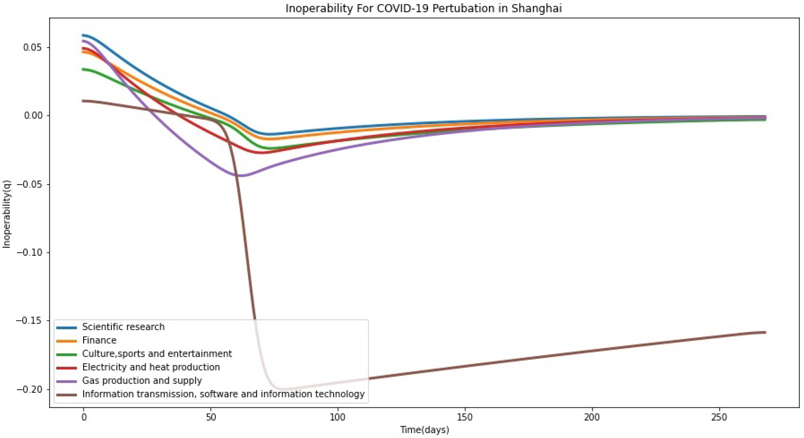
There are some other sectors, as shown in Figure 2, such as scientific research (S34); Finance (S31); culture, sports, and entertainment (S35); electricity and heat production (S23); gas production and supply (S24); information transmission, software and information technology (S30) the degree of inoperability declined steadily until it reached around 60th day and then recovered to an assumption ultimate inoperability degree of approximately 0.01 value. Unlike other sectors, the inoperability of these industries is negative. First, the difference between the actual and planned output production $(\widehat{x}-\stackrel{\sim }{x})$ for these sectors is negative, indicating that the pandemic did not have a negative effect, but rather contributed to their growth; second, the dependent between sector itself and other sectors, particularly those with higher inoperability rankings, are generally low, signifying that the negative indirect influence is smaller than the positive direct impact. The causes underlying this pattern have significant implications in practical terms, the Shanghai Municipal Bureau of Statistics data showed information transmission, software, and information technology (S30) experienced 5.3% substantial growth in the first half year and 6.1% in finance (S31), this growth has the same meaning with negative inoperability value [1]. At the beginning of COVID-19 in Shanghai, culture, sports, and entertainment (S35) was immediately impacted, but with the fast expansion of the internet and digital economy industries, the entertainment and cultural industries have achieved precise offline and online docking. Although the policy of lockdown implemented at the beginning of the pandemic restricted the development of entertainment and cultural industrial entity, it also drastically raised the demand for online material, which helped to counteract the negative impact of COVID-19 and brought about positive growth. Similarly, the scientific research (S34) has comparable practical significance. In conclusion, in the processing of the DIIM model, the research adopted a phased non-linear effect model which divided the Shanghai pandemic into two stages and put the 60th day as a dividing line in accordance with the Shanghai government’s policy for controlling the pandemic. The period of silence lasted 60 days in the first stage, and the period of release and return to work lasted 210 days after that. Such phased expressions of the recovery of various departments are also truer to the actual world. Dynamic analysis is therefore beneficial for evaluating the possible impact of the pandemic from two perspectives: the immediate direct impact of the originally interrupted sector, and the indirect chain impact on other interdependent economic sectors.

5.2. Economic Loss Analysis

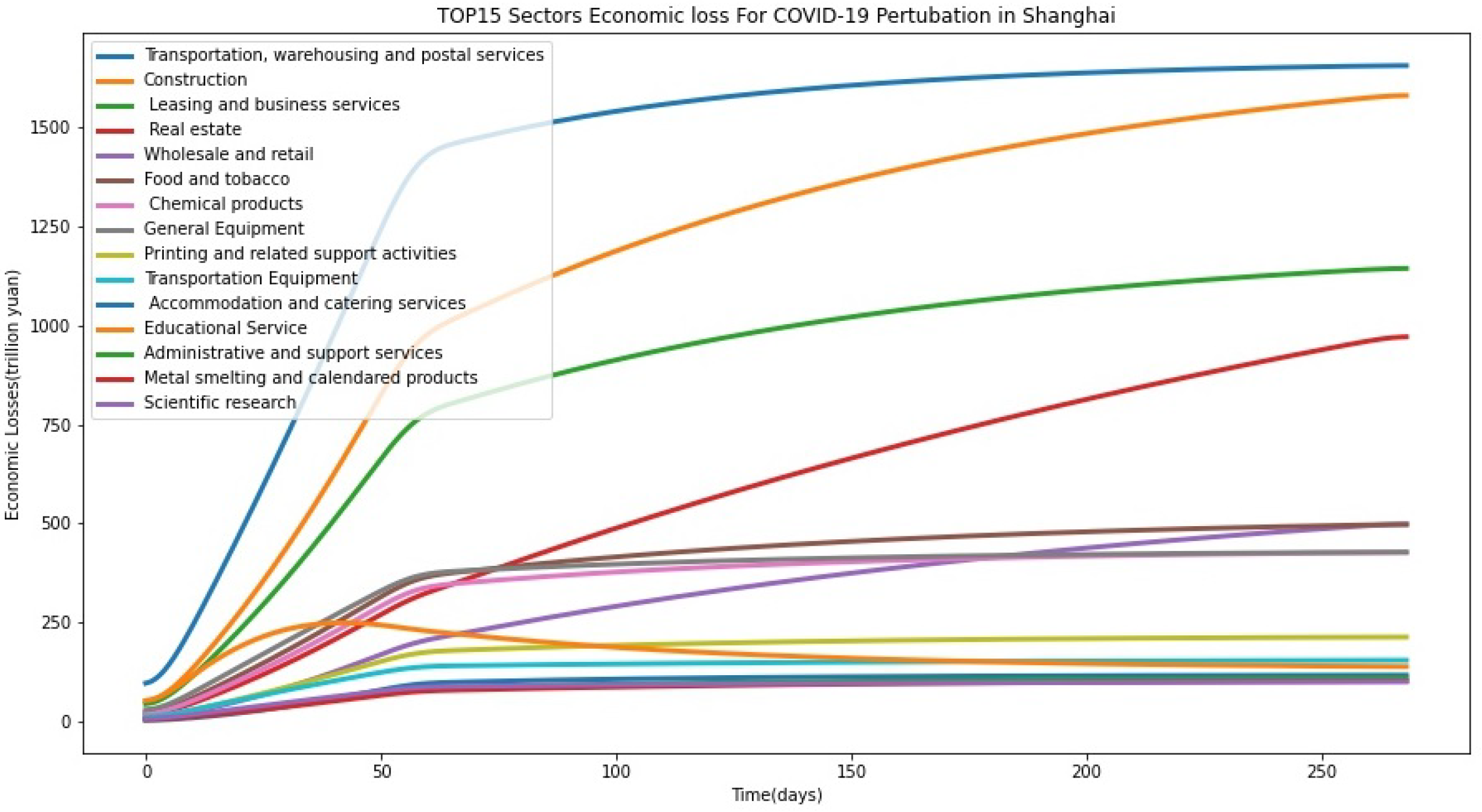
Figure 3 illustrates the real impact of the shock in terms of economic losses in greater detail. As depicted in the graph, the Top 15 industries with the most accumulated economic losses during the 120 days are transportation, warehousing, and postal (S28); construction (S26); leasing and business services (S33); real estate (S32); wholesale and retail (S27); food and tobacco (S55); chemical products (S11); general equipment (S15); printing and related support activities (S9); transportation equipment (S17); accommodation and catering services (S29); educational service (S38); administrative and support services (S37); metal smelting and calendared products (S13); scientific research (S34).

In terms of total volumes, Shanghai’s total economic loss is 0.718 trillion yuan, with losses in the primary, secondary, and tertiary industries totaling 0.010, 0.360, and 0.348 trillion yuan, respectively. Eight of the top fifteen sectors were part of the tertiary economy, while the remaining seven were considered to be part of the secondary economy. Economic losses in the transportation, warehousing, and postal (S28); construction (S26); leasing and business services (S33); real estate (S32); wholesale and retail (S27) exceeded 0.55 trillion yuan and accounted for 81.7% of the total economic loss. The top 15 sectors collectively suffered economic losses of 0.816 trillion yuan which demonstrates that the acceleration of the restart of production in these key industries is essential to the complete recovery of Shanghai’s economy. The total economic loss of the top 15 sectors is higher than 0.718 trillion yuan because there are still some sectors that have experienced positive growth during the pandemic and have not suffered economic losses.

According to the data on economic loss, not all sectors in Shanghai have generated economic losses. During the era of pandemic prevention and control, the following industries, nevertheless, saw positive growth, which went as high as 0.186 trillion yuan. These industries are gas production and supply (S24); finance (S31); information transmission, software, and information technology (S30). This is in line with the data from the Municipal Bureau of Statistics of Shanghai that growth was achieved during the pandemic [1]. During the outbreak, for instance, the information transmission, software, and information technology (S30) industry grew by 0.177 trillion yuan. From the inoperability changing view, in Figure 2 the degree to which it had a direct influence on the communication industry in the early stage of COVID-19 plummeted to a negative value. Although it rebounded later, the inoperability has always been negative until T = 210 days. This occurrence is not difficult to comprehend. On the one hand, the sector is expected to feel a moderate amount of disruption because of the outbreak. With the assistance of sophisticated networks and communication infrastructure, the online office has no impact on the value creation of most industry organizations. On the other hand, telecommuting and teleconferencing have continually evolved in modern life, and the transition from traditional brick-and-mortar offices to revolutionary virtual offices has resulted in an enormous rise in the volume of Internet traffic. Additionally, a similar tendency of inoperability has been noticed in other industries either, which is completely commensurate with the law of real-world economic operation. Moreover, in the gas production and supply (S24), the pandemic has not significantly reduced the development of such secondary industries but has finally had a positive effect on them. Moreover, some negative inoperability sectors, such as scientific research (S34); electricity and heat production (S23), not only failed to achieve economic growth but also experienced economic losses. Since cumulative economic loss depends on two factors: sector inoperability and total output. As the preceding analysis, economic losses encompass not just the sector’s direct losses, but also the effect of other sectors on the sector. If a sector is unduly dependent on the sector with a greater economic loss (high inoperability, high output production, or a combination of the two), and the indirect economic loss transmitted to the sector surpasses the sector’s economic growth, a negative inoperability with economic losses will ensue.

5.2.1. Multi-Criteria Evaluation

Figure 1 and Figure 3 show the time-varying change path of the top 15 sectors’ inoperability and economic loss value.

Table 3. Table list of Top 15 sectors most affected in terms of inoperability given demand-side COVID-19 perturbation in Shanghai.

Sector Index	Sector Name	Inoperability	Rank
S26	Construction	0.86543	1
S55	Food and tobacco	0.41702	2
S38	Educational Service	0.30833	3
S28	Transportation, warehousing and postal	0.29914	4
S32	Real estate	0.26451	5
S12	Non-metallic mineral products	0.25431	6
S33	Leasing and business services	0.24850	7
S37	Administrative and support services	0.24534	8
S6	Textile mills products	0.17618	9
S0	Forestry, fishing and related activities	0.17051	10
S14	Metal products	0.14373	11
S29	Accommodation and catering services	0.13769	12
S15	General Equipment	0.12038	13
S22	Repair services for metal products, machinery, and equipment	0.11124	14
S25	Water production and supply	0.10534	15

Note: data were obtained from the authors’ calculations.

and

Table 4. Table list of Top 15 sectors most affected in terms of economic loss value given demand-side COVID-19 perturbation in Shanghai.

Sector Index	Sector Name	Economic Loss (Trillion Yuan)	Rank
S28	Transportation, warehousing and postal	0.16580	1
S26	Construction	0.15857	2
S33	Leasing and business services	0.11469	3
S32	Real estate	0.09795	4
S27	Wholesale and retail	0.05013	5
S55	Food and tobacco	0.04984	6
S11	Chemical products	0.04282	7
S15	General Equipment	0.04274	8
S9	Printing and related support activities	0.02133	9
S17	Transportation Equipment	0.01546	10
S29	Accommodation and catering services	0.01385	11
S38	Educational Service	0.01171	12
S37	Administrative and support services	0.01095	13
S13	Metal smelting and calendared products	0.01022	14
S34	Scientific research	0.01006	15

Note: data were obtained from the authors’ calculations.

illustrate the inoperability level and final cumulative economic loss for these 15 sectors. From a comparative perspective, 10 sectors appear in the both top 15 for inoperability and economic losses sectors: transportation, warehousing, and postal (S28); construction (S26); leasing and business services (S33); real estate (S32); food and tobacco (S55); general equipment (S15); transportation equipment (S17); accommodation and catering services (S29); educational service (S38); administrative and support services (S37). These industries had significant economic volumes and workforce losses (a high proportion of labor compensation value added), as a result, each sector has relatively high sector rankings in terms of interoperability degree and economic loss.

When mentioning the disparities in inoperability and economic loss indicators, the rankings also differ across sectors, the primary reason is that production outputs of the sectors could vary by orders of magnitude. When tracking back to the DIIM equation, if a sector with a lower level of output in comparison to other sectors, but experienced significant levels of inoperability as the lockdown has progressed, this sector may have the opposite ranking levels on these two indicators, with a lower economic loss value and a higher degree of inoperability. While, a greater economic scale does not necessarily indicate a greater degree of inoperability and economic loss value, which is mostly determined by the labor loss in various industries. For instance, healthcare and social service (S39) has a higher reliance on labor than other industries, the lower production level does not preclude the possibility of higher inoperability ranking [43]. In conclusion, these studies have significant repercussions for risk management. On the one hand, the Shanghai government needs to place a larger priority on the revival of industries that suffered greater economic losses. On the other hand, when merely the degree of inoperability is utilized as a criterion for priority, there is a risk of omitting industries that have experienced significant economic losses. Consequently, this idea needs to be evaluated in greater depth. As a result, these two indicators can only provide a gauge of how departments should be prioritized. When prioritizing and restoring departments, further decision-making techniques are required to assess the balance between economic losses and inoperability with greater precision.

5.2.2. Compared with Published Results

Since the outbreak in Shanghai of COVID-19 was relatively close to the writing time of the paper, there are no articles or official statistics on the overall economic loss of the Shanghai pandemic. Only some authoritative editors have made basic estimates of economic losses from different angles. Guoshu Zhan believes that through the statistics of direct costs such as living material expenditures and medical material expenditures, and indirect costs such as industrial production and government markets, the final cost of confinement is 0.75 trillion yuan [44]. There are also other editors who estimate from the perspective of GDP and obtain about 0.64 trillion yuan Economic losses [44]. This is basically close to the estimated result of 0.718 trillion yuan in this paper.

5.3. Risk Management Scenario Analysis

The government has declared several times to identify the importance of a risk management system to prevent the COVID-19 cascading effect. Through the DIIM model, the economic loss can be assessed to help policymakers in decision making. The analysis of risk assessment management is necessary for our research paper. Through previous analysis, it is clear that there is an imbalance ranking between inoperability and economic loss, therefore such a risk management trade-off method can make the paper figure out the balance in terms of costs, benefits, and risks and the impact of current action and future influence [45,46]. This section discusses three scenario cases based on the surrogate worth trade-off method for evaluating the efficacy of risk management options that can reduce the economic loss effects of risk management options [6,47].

Assume that the government will prefabricate part of the investment cost from the 2022 government budget in advance to prevent and control the damage to the economy when the uncontrollable pandemic spreads. The investment cost of the risk management policy will be obtained from the Municipal Health Commission of Shanghai [48]. According to the 2022 departmental budget of the Municipal Health Commission of Shanghai, it can be seen that the financial budget of the commission in 2022 is 4.503 billion yuan, of which 1.814 billion yuan is used for public health and 96 million yuan is used for disease prevention and control. The paper selects the sum of these two data which is 2.72 billion yuan as the investment cost.

Scenario 1: assume adopt no risk management policy (set policy option $j=0$)

In the first hypothetical scenario, assume that policy option $j=0$, that is, no risk management measures are taken, and all inoperability and economic losses come from the calculation of the DIIM model result in this paper the outbreak of the Shanghai pandemic, which is the real shock occurrence under the DIIM model. Therefore, the economic loss after taking risk management is equal to the economic loss without taking management measures and the execution cost is 0. At the same time, we set scenario 1 as the baseline scenario to facilitate subsequent analysis:

$${{\delta }_j={\Gamma }_{w\left[0\right]}-\Gamma }_{w\left[j\right]}-{\gamma }_j=0trillionyuan$$

(40)

Scenario 2: assume adopt risk management policy (set policy option $j=1$)

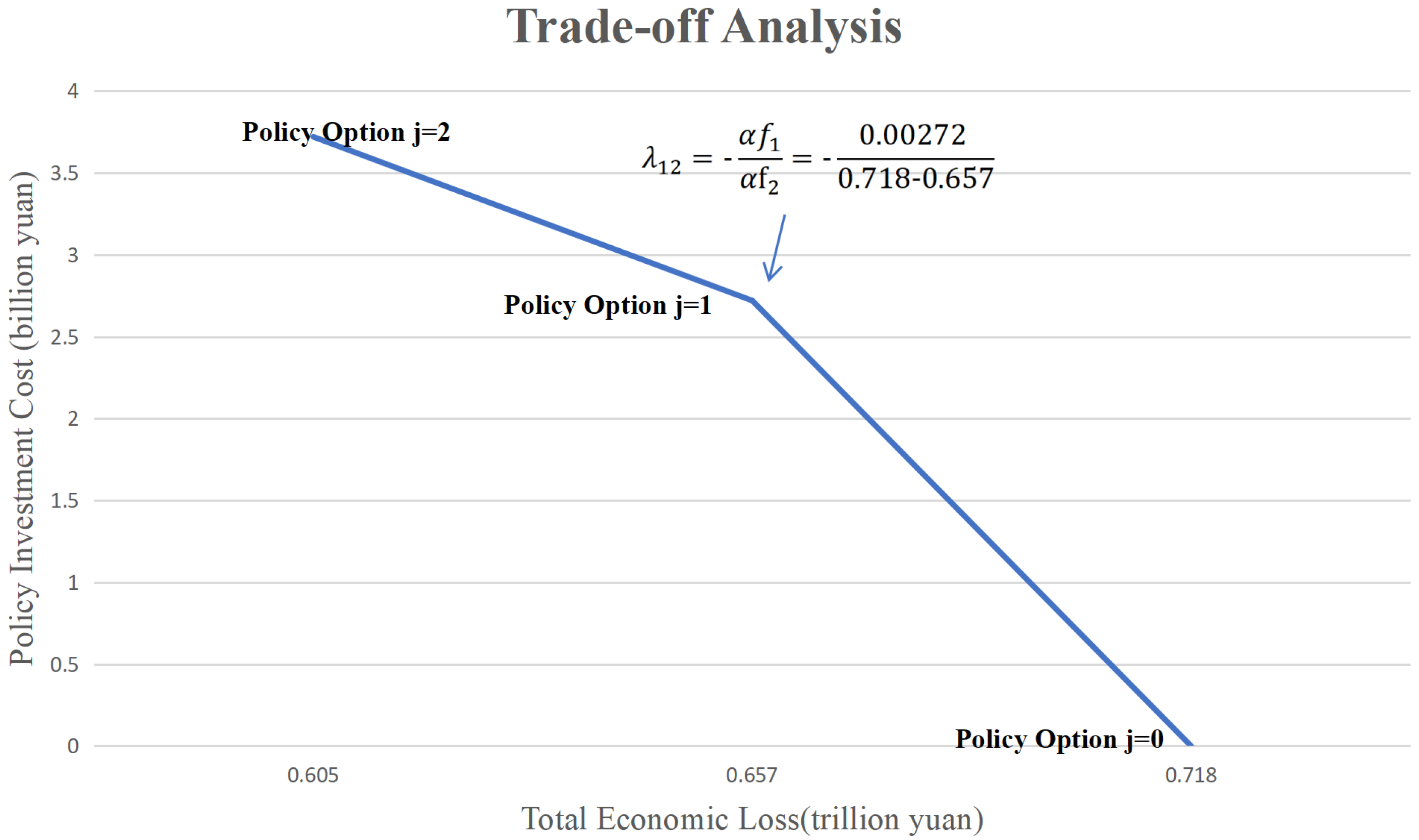
In this scenario, the paper assumed risk management policy 1 that the government will spend 2.72 billion yuan in advance for risk control to prevent the impact of the sudden spread of the pandemic on the economic system as much as possible. Moreover, suppose that this advanced risk management policy will reduce the impact of the pandemic by 5% every day, and when it acts on the inoperability level, it will only suffer the impact of the 95% degree of original inoperability level each day. Bringing the changed degree of inoperability back into the DIIM model for further analysis, it is found that under the implementation of risk management policy 1, the overall economic loss is 0.657 trillion yuan, compared with the previous loss of 0.718 trillion yuan, the overall loss is reduced by 0.061 trillion yuan. Therefore, the net benefit is 0.0583 trillion yuan, and the cost-benefit ratio is 0.045. The specific calculation results are as follows:

$${{\delta }_1={\Gamma }_{w\left[0\right]}-\Gamma }_{w\left[1\right]}-{\gamma }_1=0.718-0.657-0.00272=0.0583trillionyuan$$

(41)

$${\lambda }_{12}=\frac{{\gamma }_1}{{{\Gamma }_{w\left[0\right]}-\Gamma }_{w\left[1\right]}}=\frac{0.00272}{0.718-0.657}=0.045$$

(42)

Scenario 3: assume adopt risk management policy (set policy option $j=2$)

Based on risk management policy 2, it assumed that an additional 1 billion yuan investment cost will be added to the expenditure of early prevention and control, resulting in a total investment cost of 3.72 billion yuan. This approach is to prevent the current and future cascading effects of a wider pandemic on Shanghai and to predict the current year’s budget in advance for risk prevention and control. Based on this, the paper wants to calculate the impact of the additional 1 billion yuan of investment cost on the impact of the Shanghai pandemic, assuming that this additional expenditure cost will reduce the recovery time after Shanghai’s lockdown period from the initial 60 days to 30 days. If this additional spending can reduce the time for Shanghai to return to normal market activities by one month, repeating the steps of the DIIM model, the overall economic loss will be reduced from 0.718 trillion yuan without risk management measures to 0.605 trillion yuan. Therefore, the net benefit is 0.076 trillion yuan, the cost-benefit ratio is 0.033. The specific calculation process is as follows:

$${{\delta }_2={\Gamma }_{w\left[0\right]}-\Gamma }_{w\left[2\right]}-{\gamma }_2=0.718-0.605-0.00372=0.109trillionyuan$$

(43)

$${\lambda }_{12}=\frac{{\gamma }_2}{{{\Gamma }_{w\left[0\right]}-\Gamma }_{w\left[2\right]}}=\frac{0.00372}{0.718-0.605}=0.033$$

(44)

Visualize the trade-off values of different risk management policies and display a risk management trade-off analysis diagram. The abscissa is the cumulative economic loss $\left(f_1\right)$ under different risk management policies, and the ordinate is the policy implement cost $\left(f_2\right)$. The slope of the graph is the LaGrange multiplier, which allows policymakers to measure the possible return under different policy measures. The previous three hypothetical scenarios are drawn in Figure 4, and from scenario 2, it can be found that ${\lambda }_{12}$ shows the ratio of 2.72 billion yuan $\left(f_1\right)$ cumulative economic loss respect to economic loss reduction. This method of measuring policy implementation efficiency can be applied to different policy programs, as long as the economic loss under DIIM and the investment cost of the policy are determined. When conducting a cost-benefit-risk analysis, SWT may intuitively inform the policymaker of the loss ratio and allow them to make the final decision based on their financial budget and risk-taking capacity. As can be seen from the figure, the essence of the Lagrange multiplier is the cost-benefit ratio which indicates that the risk control management estimated benefits significantly outweigh its costs if the number is less than 1. For the risk control management 1, the ${\lambda }_{12}$ is 0.045 which indicates the government could obtain 1 yuan of benefit for each 0.045 yuan of investment cost. As with risk management policy 2, in which the ${\lambda }_{12}$ is 0.325, the government could obtain 1 yuan of benefit for each 0.033 yuan of investment cost. Compared with these two policies, the second risk management measure is better, that is, it has a smaller investment cost under the unit benefit, even if it takes 1 billion yuan investment cost more than the first policy.

6. Summary and Conclusions

This paper proposes a systematic analysis method for analyzing the risks of the system created by disturbances caused by natural disasters, economic losses, and government policies. The overall idea is to establish a demand-side DIIM model, and analyze and manage risk associated with the pandemic in Shanghai in the first half of 2022 from the perspective of final production output. Although the pandemic has brought serious negative impacts on social life, this paper provides a basic framework for predicting and evaluating similar events in the future, conducts accurate risk assessment of possible complex system failures, provides policymakers with potential solution plans, and achieves a balance of cost, benefit, and risk. The innovation of this paper is that compared with the negative shocks produced by other papers, this paper analyzes the economic sectors with positive growth under the pandemic.

The DIIM model is based on Shanghai’s 2017 input–output table which provides a guarantee for the reliability and authenticity of the data and provides a solid foundation for the analysis of subsequent disaster losses caused by the pandemic. Combined with the ‘input–output relationship’ of each sector in the input–output table, the most vulnerable sectors can be acquired and provide a guarantee for subsequent decision-makers to formulate policies. While the DIIM model unlike the traditional static model, not only performs mathematical calculations on the results after the disaster but also performs time-series display analysis on the inoperability of disaster and changes in losses. Different from the one-time calculation of the degree of loss caused by the traditional I-O table, the loss of DIIM is based on the accumulation process of inoperability degree changes, so the value calculated by DIIM is often larger than the result of the I-O table and closer to the real situation. In this case result, the DIIM model provides reliable results for the event analysis of the impact of the pandemic and combines the sectoral Leontief coefficient of the input–output table to determine the degree of inoperability and economic losses under the impact. The 0.718 trillion yuan estimated in this paper is relatively consistent with the results of 0.64 or 0.75 trillion yuan estimated by other scholars at the same time [44]. The DIIM model not only displays the total loss, but also demonstrates the situation of the sub-departments, and according to the Leontief coefficient between the various departments in the input–output table, it is convenient to conduct investigations one by one to determine the impact of the event. When conducting the case study, the results show that the rankings of departments in terms of inoperability and economic loss are different. Therefore, it is necessary to look at the final result dialectically. In decision-making, inoperability indicates the degree of loss of a sector under a disaster, that is, vulnerability. The economic loss is based on the economic benefit under the quantified loss of inoperability and sectoral production output. Therefore, it is particularly important to balance the magnitude of monetary loss (economic loss), as well as the relative impact on the size of the sector (i.e., inoperability). At the same time, in order to manage risks more effectively, policymakers must recognize the trade-offs between risks and resources. For example, in order to reduce the impact of the pandemic on the economy, the government can consider how to achieve precise prevention and control in advance to prevent wider spread. Allocation issues can also be addressed through sensitivity analysis and uncertainty analysis. This paper uses SWT to represent risk management measures and analyzes the trade-off analysis under the three scenarios of original shock, inoperability shock reduction, and recovery event shortening. The Lagrange multiplier of SWT can show the cost-benefit ratio of government investment costs and policy benefits. When this value is less than 1, it means that the government risk management policy is effective. This paper selects three scenarios for analysis, among which risk management policy 2 has a lower cost-benefit ratio on the premise that the investment cost is 1 billion yuan more than policy 1, that is, 1 unit of benefit requires less spending, so it is more economical. The limitation of the paper is that based on the availability of data, the hysteresis of the input–output table, and the duration of the case, this paper only analyzes the pandemic situation from the perspective of the demand side; however, the pandemic will not only affect the demand side but also the supply side. Therefore, it is only a preliminary discovery of a specific case. Further in-depth research can be conducted simultaneously from the perspectives of supply and demand, and other external factors such as institutional formulation and market changes will lead to more complex changes.

References

1. Municipal Bureau of Statistics of Shanghai. Shanghai’s GDP in the First Half of 2022. 2022. Available online: https://tjj.sh.gov.cn/ydsj2/20220719/cb29bc2eb997465faddc45e59ab31cf6.html (accessed on 9 January 2023).
2. Cochrane, H.C. Predicting the economic impact of earthquakes. In Social Science Perspectives on the Coming San Francisco Earthquake, Natural Hazards Research Paper; Institute of Behavioral Science, University of Colorado: Boulder, CO, USA, 1974; Volume 25. [Google Scholar]
3. Kousky, C. Informing climate adaptation: A review of the economic costs of natural disasters. Energy Econ. 2014, 46, 576–592. [Google Scholar] [CrossRef]
4. Skidmore, M.; Toya, H. Do natural disasters promote long-run growth? Econ. Inq. 2002, 40, 664–687. [Google Scholar] [CrossRef]
5. Haimes, Y.Y. Risk Modeling, Assessment, and Management; John Wiley & Sons: Hoboken, NJ, USA, 2005; Volume 615, p. 7. [Google Scholar]
6. Santos, J. Using input-output analysis to model the impact of pandemic mitigation and suppression measures on the workforce. Sustain. Prod. Consum. 2020, 23, 249–255. [Google Scholar] [CrossRef]
7. Tatar, U.; Santos, J.R.; Thekdi, S.A. Managing Physical and Economic Risk for Systems with Multidirectional Network Interdependencies. Risk Anal. 2022, 42, 1106–1123. [Google Scholar] [CrossRef]
8. He, K.; Mi, Z.; Coffman, D.M.; Guan, D. Using a linear regression approach to sequential interindustry model for time-lagged economic impact analysis. Struct. Chang. Econ. Dyn. 2022, 62, 399–406. [Google Scholar] [CrossRef]
9. Avelino, A.F.; Dall’erba, S. Comparing the economic impact of natural disasters generated by different input–output models: An application to the 2007 Chehalis river flood (wa). Risk Anal. 2019, 39, 85–104. [Google Scholar] [CrossRef] [Green Version]
10. Huang, Y.; Chen, C. Impacts of COVID-19 on China’s Economic System Based on Dynamic Inoperability Input-output Model. J. Syst. Manag. 2021, 30, 1152–1158. [Google Scholar]
11. El Haimar, A.; Santos, J.R. A stochastic recovery model of influenza pandemic effects on interdependent workforce systems. Nat. Hazards 2015, 77, 987–1011. [Google Scholar] [CrossRef]
12. Santos, J.; Roquel, K.I.D.Z.; Lamberte, A.; Tan, R.R.; Aviso, K.B.; Tapia, J.F.D.; Solis, C.A.; Yu, K.D.S. Assessing the economic ripple effects of critical infrastructure failures using the dynamic inoperability input-output model: A case study of the Taal Volcano eruption. Sustain. Resil. Infrastruct. 2022, 23, 68–84. [Google Scholar] [CrossRef]
13. Ghosh, A. Input-output approach in an allocation syste m. Economica 1958, 25, 58–64. [Google Scholar] [CrossRef]
14. Leung, M.; Haimes, Y.Y.; Santos, J.R. Supply-and output-side extensions to the inoperability input-output model for interdependent infrastructures. J. Infrastruct. Syst. 2007, 13, 299–310. [Google Scholar] [CrossRef]
15. Xu, W.; Hong, L.; He, L.; Wang, S.; Chen, X. Supply-driven dynamic inoperability input-output price model for interdependent infrastructure systems. J. Infrastruct. Syst. 2011, 17, 151–162. [Google Scholar] [CrossRef]
16. Ocampo, L.; Masbad, J.G.; Noel, V.M.; Omega, R.S. Supply-side inoperability input–output model (SIIM) for risk analysis in manufacturing systems. J. Manuf. Syst. 2016, 41, 76–85. [Google Scholar] [CrossRef]
17. Oosterhaven, J. On the limited usability of the inoperability IO model. Econ. Syst. Res. 2017, 29, 452–461. [Google Scholar] [CrossRef] [Green Version]
18. Brucker, S.M.; Hastings, S.E.; Latham, W.R., III. The variation of estimated impacts from five regional input-output models. Int. Reg. Sci. Rev. 1990, 13, 119–139. [Google Scholar] [CrossRef]
19. Lian, C.; Haimes, Y.Y. Managing the risk of terrorism to interdependent infrastructure systems through the dynamic inoperability input–output model. Syst. Eng. 2006, 9, 241–258. [Google Scholar] [CrossRef]
20. Leontief, W. Input-Output Economics; Oxford University Press: Oxford, UK, 1986. [Google Scholar]
21. Santos, J.R.; Haimes, Y.Y. Modeling the demand reduction input-output (I-O) inoperability due to terrorism of interconnected infrastructures. Risk Anal. Int. J. 2004, 24, 1437–1451. [Google Scholar] [CrossRef]
22. Haimes, Y.Y.; Jiang, P. Leontief-based model of risk in complex interconnected infrastructures. J. Infrastruct. Syst. 2001, 7, 1–12. [Google Scholar] [CrossRef]
23. Jiang, P.; Haimes, Y.Y. Risk management for Leontief-based interdependent systems. Risk Anal. Int. J. 2004, 24, 1215–1229. [Google Scholar] [CrossRef]
24. Dietzenbacher, E. In vindication of the Ghosh model: A reinterpretation as a price model. J. Reg. Sci. 1997, 37, 629–651. [Google Scholar] [CrossRef]
25. Oosterhaven, J. On the plausibility of the supply-driven input-output model. J. Reg. Sci. 1988, 28, 203–217. [Google Scholar] [CrossRef]
26. Zaghini, E. Solow Prices and the Dual Stability Paradox in the Leontief Dynamic System. Econometrica 1971, 39, 153. [Google Scholar] [CrossRef]
27. Davar, E. Price Discrimination in Input–Output. Econ. Syst. Res. 1993, 5, 3–10. [Google Scholar] [CrossRef]
28. Ramos Carvajal, M.D.C.; Blanc Díaz, M. The Foundations of Dynamic Input-Output Revisited: Does Dynamic Input-Output Belong to Growth Theory? Documentos de trabajo; Universidad de Oviedo, Facultad de Ciencias Económicas: Oviedo, Spain, 2002. [Google Scholar]
29. Liew, C.J. The dynamic variable input-output model: An advancement from the Leontief dynamic input-output model. Ann. Reg. Sci. 2000, 34, 591–614. [Google Scholar] [CrossRef]
30. Haimes, Y.Y. Hierarchical holographic modeling. IEEE Trans. Syst. Man Cybern. 1981, 11, 606–617. [Google Scholar] [CrossRef]
31. Sharland, M.; Gattinara di Zub, G.C.; Tomas Ramos, J.; Blanche, S.; Gibb, D.M.; PENTA Steering Committee. PENTA guidelines for the use of antiretroviral therapy in paediatric HIV infection. HIV Med. 2002, 3, 215–226. [Google Scholar] [CrossRef]
32. Edwards, C.H.; Penney, D.E. Differential Equations and Boundary Value Problems: Computing and Modeling; Pearson Educación: London, UK, 2000. [Google Scholar]
33. Okuyama, Y.; Yu, K.D. Return of the inoperability. Econ. Syst. Res. 2019, 31, 467–480. [Google Scholar] [CrossRef]
34. Municipal Bureau of Statistics of Shanghai. Gross Output Value of Industrial Enterprise above Designated Size (by Industry). 2022. Available online: https://tjj.sh.gov.cn/ydsj32/index.html (accessed on 9 January 2023).
35. Municipal Bureau of Statistics of Shanghai. Gross Output Value of Tertiary Industry above Designated Size (by Industry). 2022. Available online: https://tjj.sh.gov.cn/ydsj102/index.html (accessed on 9 January 2023).
36. Rose, A.; Liao, S.Y. Modeling regional economic resilience to disasters: A computable general equilibrium analysis of water service disruptions. J. Reg. Sci. 2005, 45, 75–112. [Google Scholar] [CrossRef]
37. Okuyama, Y.; Sonis, M.; Hewings, G.J. Economic impacts of an unscheduled, disruptive event: A Miyazawa multiplier analysis. In Understanding and Interpreting Economic Structure; Springer: Berlin/Heidelberg, Germany, 1999; pp. 113–143. [Google Scholar] [CrossRef]
38. MacKenzie, C.A.; Santos, J.R.; Barker, K. Measuring changes in international production from a disruption: Case study of the Japanese earthquake and tsunami. Int. J. Prod. Econ. 2012, 138, 293–302. [Google Scholar] [CrossRef]
39. Burrus, R.T., Jr.; Dumas, C.F.; Farrell, C.H.; Hall, W.W., Jr. Impact of low-intensity hurricanes on regional economic activity. Nat. Hazards Rev. 2002, 3, 118–125. [Google Scholar] [CrossRef]
40. National Bureau of Statistics of China. Shanghai’s Urban Unemployment Rate in the Second Quarter of 2022. 2022. Available online: http://www.stats.gov.cn/tjsj/sjjd/202207/t20220715_1886475.html (accessed on 9 January 2023).
41. Santos, J.R.; Orsi, M.J.; Bond, E.J. Pandemic recovery analysis using the dynamic inoperability input-output model. Risk Anal. Int. J. 2009, 12, 1743–1758. [Google Scholar] [CrossRef]
42. Municipal Bureau of Statistics of Shanghai. Shanghai City Accelerated Economic Recovery and Revitalization Plan. 2022. Available online: https://www.jinshan.gov.cn/yszc-gjshsyszc/20220529/830938.html (accessed on 9 January 2023).
43. Akhtar, R.; Santos, J.R. Risk-based input–output analysis of hurricane impacts on interdependent regional workforce systems. Nat. Hazards 2013, 65, 391–405. [Google Scholar] [CrossRef]
44. Wangyi. How High Is the Cost of Shanghai’s Pandemic Containment? Available online: https://www.163.com/dy/article/H87MVPAV05534DWL.html (accessed on 9 January 2023).
45. Hayes, J.L. Record Floods of Greater Nashville: Including Flooding in Middle Tennessee (TN) and Western Kentucky (KY), May 674 1-4-2010: Service Assessment; DIANE Publishing: Collingdale, PA, USA, 2011. [Google Scholar]
46. Yu, K.D.S.; Aviso, K.B. Modelling the economic impact and ripple effects of disease outbreaks. Process Integration and Optimization for Sustainability. Process Integr. Optim. Sustain. 2020, 4, 183–186. [Google Scholar] [CrossRef] [Green Version]
47. Santos, J. Reflections on the impact of “flatten the curve” on interdependent workforce sectors. Environ. Syst. Decis. 2020, 40, 185–188. [Google Scholar] [CrossRef]
48. Municipal Health Commission of Shanghai. Report on Departmental Budget of Shanghai Municipal Health Commission in 2022. 2022. Available online: https://wsjkw.sh.gov.cn/czgk/20220215/543c8e61f7864f58ae18d49b16e123bc.html (accessed on 9 January 2023).
Figure 1. Top 15 sectors most affected in terms of inoperability given demand-side COVID-19 perturbation in Shanghai.
Sustainability 15 04003 g001
Figure 2. Negative value sectors in terms of inoperability given demand-side COVID-19 perturbation in Shanghai.
Sustainability 15 04003 g002
Figure 3. Top 15 sectors most affected in terms of economic loss given demand-side COVID-19 perturbation in Shanghai.
Sustainability 15 04003 g003
Figure 4. SWT trade−off analysis given demand−side COVID−19 perturbation in Shanghai.
Sustainability 15 04003 g004