Abstract
With rapid urbanization and increasingly prominent environmental issues, objective evaluation of the quality of the ecological environment is crucial for environmental protection and sustainable development. Most remote sensing ecological indices (RSEI) used for ecological environmental quality evaluation include only four indicators (greenness, humidity, heat, and dryness), and many studies have ignored the impact of air quality on urban ecological environmental quality in arid areas. This study used the urban agglomeration on the northern slope of the Tianshan Mountains (UANSTM), China, as the research area based on the Google Earth Engine platform via Landsat remote sensing images and NPP/VIIRS data to establish a new remote sensing ecological index (RSEInew) and compounded night light index of urbanization level. The coupling coordination degree model was used to quantitatively analyze the characteristics of the coordinated development of the ecological environment and urbanization in UANSTM and major cities from 2015 to 2020. The results showed that: (1) compared to RSEI, RSEInew is more suitable for assessing the ecological quality of arid zones because it accounts for air quality; (2) the RSEInew value for the eco-environmental quality of UANSTM from 2015 to 2020 improved and then deteriorated with an overall declining trend. The variation in the RSEInew rating was between “strongly bad” and “neutral,” and there were differences in the quality of the ecological environments among cities; (3) the level of urbanization in the economic zone of UANSTM from 2015 to 2020 increased significantly, and the degree of coordination between urbanization and ecological environmental quality coupling steadily increased but remained moderately imbalanced. The results of this study provide a scientific reference for the economic development and ecological environmental protection of the study area.
1. Introduction
The quality of the ecological environment refers to the extent by which the ecological environment affects human survival and social and economic development within a certain time and space and is the basic attribute of the ecological environment [1,2]. Urbanization is an inevitable process of human progress and has become a major factor that exerts continuous pressure on the natural environment and is thus an issue of global concern [3,4]. A complex interaction exists between urbanization and ecological environmental quality. High-intensity urbanization interferes with and destroys the ecological environment, and the deterioration of the ecological environment restricts urbanization and sustainable development [5,6]. For ecologically fragile arid areas, it is particularly important to research ecological environmental quality and discuss how to coordinate the relationship between economic development and the ecological environment.
Remote sensing technology provides the means for rapid, real-time, and large-scale monitoring [7,8] and has been widely used in ecological monitoring and evaluation [9,10,11]. Some studies have evaluated the growth of forest communities using vegetation indices from remote sensing inversion [12], the urban heat island effect using land surface temperature [13], and the quality of the urban ecological environment by analyzing urban impervious surfaces extracted by remote sensing technology [14]. However, the formation and development of ecosystems are influenced by a variety of factors. Further, to a certain extent, a single indicator cannot fully reflect the real situation of natural processes. Xu proposed a remote sensing ecological index (RSEI) constructed using multiple indicators [15], which has been widely used at different scales and in multiple fields [16,17]. The RSEI should be appropriately improved when analyzing specific regions with different ecological conditions. Some studies have established RSEIs based on moving windows and considering the impact of mining areas on the ecological environment [18], while others have improved the RSEI by selecting the principal components and setting the weight [19]. However, air quality is an important factor affecting the urban environment, with particulate matter posing a significant impact on human respiratory and vascular systems [20]. Therefore, it is necessary to integrate air quality data into ecological evaluations.
Nighttime light (NTL) data are widely used in research on human activities and urban development [21,22]. Socio-economic statistic indicators for overall regional analysis have been used by studies investigating the relationship between urbanization and the ecological environment [23,24,25,26]. With the development of remote sensing technology providing new ways to investigate both, some studies have used the compounded nighttime light index (CNLI), which represents the level of urbanization, to analyze the coupling coordination relationship between urbanization and the ecological environment [27]. Arid areas are vast and ecologically fragile, and with the rapid expansion of cities, there is bound to be an impact on the environment; therefore, the use of remote sensing technology to research the coordination relationship between urbanization and the ecological environment in arid areas may be valuable. The urban agglomeration on the northern slope of the Tianshan Mountains (UANSTM) study area was one of the 19 urban agglomerations promoted by China during the “13th Five-Year Plan”.
This current study used China’s typical arid oasis UANSTM as an example. A new remote sensing ecological index (RSEInew) was constructed by introducing the particulate matter 2.5 (PM2.5) concentration difference index (DI) based on the RSEI model using the Google Earth Engine (GEE) platform via Landsat remote sensing images. NTL data were used to estimate the urbanization development indicators of the study area. Based on these results, the coupling coordination degree model (CCDM) was used to quantitatively explore the coordinated development of the ecological environment and urbanization in UANSTM from 2015 to 2020. Therefore, this study aims to: (1) construct RSEInew to monitor the spatial and temporal patterns and evolutionary trends of ecological and environmental quality in the UANSTM; (2) quantitatively analyze the coordination between ecological environment quality and urbanization levels in the arid area; and (3) analyze causes of the coupled coordination degree of ecological quality and urbanization in the study area. The results of this study have practical significance for promoting the coordinated development of urbanization and ecological environmental quality in the study area, as well as for informing environmental protection and sustainable development.
2. Materials and Methods
2.1. Study Area
UANSTM (42°45′–46°8′ N, 81°46′–88°58′ E) is the most economically developed area and an economic development center of the Xinjiang Uygur Autonomous Region in northwest China, located adjacent to the Gurbantunggut Desert to the north. It has a total area of approximately 95,400 km2, complex topography, and a temperate continental arid climate [28]. UANSTM includes the Wu-Chang urban economic zone with Urumqi City as the center, the Shihezi-Manasi-Shawan urban economic zone with Shihezi City as the center, and the Kuitun-Wusu-Kelamayi “Golden Triangle”. By incorporating various factors, such as urban development level and natural environment, this study considered Urumqi City, Shihezi City, and Kelamayi City as the axes and selected key cities in the economic belt, including Changji City, Fukang City, Kuitun City, Hutubi County, Manasi County, and Shawan County as the study area (Figure 1). UANSTM has the highest economic level, most developed transportation, densest population, and most concentrated industries in Xinjiang. At the end of 2018, the total population of the urban agglomeration was 5.92 million people, accounting for approximately a fifth of the total population of Xinjiang, with a gross domestic product of CNY 656.6 billion. This is the main area for new urbanization in Xinjiang in the future and a strategic core area for social and economic development [29].
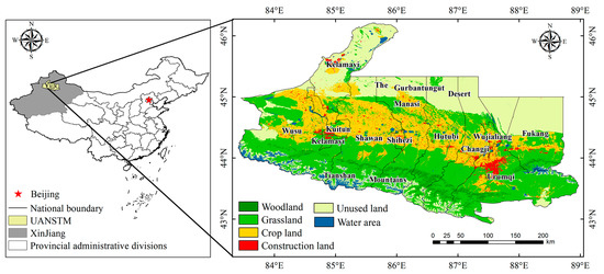
Figure 1.
Urban agglomeration on the northern slope of the Tianshan Mountains (UANSTM) location map.
2.2. Data Resources and Preprocessing
The GEE is a powerful remote sensing data source and processing platform. Using this platform, we performed batch stitching, cropping, water body masking, and other preprocessing on Landsat with 30 m spatial resolution remote sensing image data (2442 scenes) in the study area from 2015 to 2021 during three seasons (spring, summer, and autumn) each year. The greenness, humidity, heat, and dryness [30] and the PM2.5 concentration (DI) were calculated in the study area [31]. Principal component analysis (PCA) was used to build RSEInew. The NTL data in the study area from 2015 to 2020 were derived from the global “NPP-VIIRS” nighttime light time series product (https://doi.org/10.7910/DVN/YGIVCD, accessed on 17 March 2022) [32] with a spatial resolution of 500 m. Land-use data for 2015–2020 were collected from the National Earth System Science Data Center (http://www.geodata.cn/, accessed on 15 March 2022) with a spatial resolution of 30 m and reclassified into six categories: woodland, grassland, cropland, construction land, unused land, and water area (Table 1). All data and maps in this study were in the geographical coordinate system (GCS_WGS_1984).

Table 1.
Detailed descriptions of the study data.
2.3. Methods
2.3.1. New Remote Sensing Ecological Index
RSEInew was constructed by employing five ecological factors and conducting a PCA [33]. The normalized vegetation index (NDVI), wetness index (WET), land surface temperature (LST), and normalized differential built-up and bare soil index (NDBSI) represented greenness, humidity, heat, and dryness, respectively. These four ecological factors were also the main indicators for constructing conventional RSEI models [15]. This study introduced air quality as a fifth factor, namely the PM2.5 concentration DI [34,35]. The calculation formulas for all ecological factors are as follows:
- (1)
- Normalized vegetation index (NDVI)
NDVI can reflect vegetation growth and coverage in the study area [36].
- (2)
- Wetness index (WET)
WET can better reflect the water information of soil and vegetation [37,38] in the study area.
where are the reflectance of the blue, green, red, near-infrared, short infrared band1, and short infrared band2, respectively [39].
- (3)
- Land surface temperature (LST)
LST is closely related to the urban ecological environment and therefore it was used to represent the heat index [40,41,42]. In this paper, we use the thermal infra-red band of Landsat images to calculate the radiometric brightness and then the radiometric brightness is corrected according to the land surface emissivity, thus inverse performing the surface temperature.
where is the radiance of the TM (TIRS) thermal infra-red band, and gain and bias denote the band’s gain value and the offset value, respectively. Digital number (DN) is the pixel gray value; B(Ts) is the black body radiance, for Landsat5 image K1 = 607.76, K2 = 1260.56; for Landsat7 image K1 = 666.09, K2 = 1282.71; for Landsat8 image K1 = 774.89, K2=1201.14 [43]. is the center wavelength of the thermal infrared band (= 11.435 and = 10.896), = 1.438.10−2 m K, and is the land surface emissivity estimated by NDVI [40].
- (4)
- Normalized differential built-up and bare soil index (NDBSI)
The continuous expansion of the urban building land area and wide distribution of bare land around the city are factors causing soil drying in the study area and harming the regional ecological environment. Therefore, NDBSI [15,44], which is obtained via the weighted average of the soil index (SI) [15,45] and index-based built-up index (IBI) [30,46,47], was used as the dryness index to reflect the degree of drought in the study area.
where are the reflectance of the blue, green, red, near-infrared, and short infrared band1, respectively.
- (5)
- Difference index (DI)
PM2.5, the main constituent of urban pollution, is closely related to the quality of the ecological environment. The introduction of the PM2.5 concentration index can more accurately reflect the urban ecological environmental quality of the study area [33,48]. The current spatial resolution of PM2.5 concentrations estimated based on satellite remote sensing is low, and problems such as missing data often occur [35]. For this reason, many scholars have made algorithm improvements, such as Feng H.Y [34], Zha Y [31], and He J [49], who constructed indices to directly estimate PM2.5 concentrations by combining different wavebands. In this study, the difference index (DI) constructed using red and near-infrared bands was used to represent the concentration of PM2.5 as based on previous studies [33,34].
To prevent different units and numerical ranges of different ecological factors from affecting the accuracy of the RSEInew results, all indicators were normalized before constructing the RSEInew to ensure that the numerical ranges of the five factors were between 0 and 1 [50]. PCA was used to calculate the initial value of the remote sensing ecological environment index (RSEI0 = 1 − PC1). The formula for calculating the RSEInew is as follows:
where RSEI0−max and RSEI0−min are the maximum and minimum values of the initial value RSEI0, respectively. The closer RSEInew is to 1, the better the quality of the ecological environment; the closer it is to 0, the worse the quality of the ecological environment [51]. Based on previous studies on ecological environmental quality classification, the RSEInew was divided into five categories: strongly good (0.8–1.0), slightly good (0.6–0.8), neutral (0.4–0.6), slightly bad (0.2–0.4), and strongly bad (0–0.2) [52,53,54]. The annual RSEInew was calculated using the monthly scale RSEInew (with less snow cover) from March to November each year, and the monthly scale RSEInew was calculated to obtain the RSEInew of the study area at different seasonal scales.
2.3.2. Estimation of Compounded Nighttime Light Index (CNLI)
The CNLI reflects the level of urbanization and intensity of human activities on the Earth’s surface and can effectively monitor the development of regional urbanization [55]. CNLI was estimated using the light area ratio product (LAP) and mean light intensity (MLI) [56] as follows:
where Arealight represents the lighting area, Area is the total study area, is the brightness value of the ith brightness level, is the total number of pixels of the ith brightness level, and N is the total number of pixels of lights.
2.3.3. Coupling Coordination Degree Model (CCDM)
Coupling coordination analysis includes the coupling degree and coupling coordination degree analysis [57]. Coupling refers to the degree of interaction between two or more systems [58]. The coupling coordination analysis equation is as follows:
where U represents the CNLI, E represents the RSEInew, and C is the degree of interaction between urbanization and the ecological environment [59]. Owing to the coupling level, it is not possible to determine the level at which each subsystem is coordinated [60]. Therefore, based on the coupling degree, CCDM was introduced to evaluate the degree of coordinated development of the ecological environment and urbanization. The calculation formula is as follows:
where D is the degree of coupling coordination, indicating the development level of the two subsystems; the higher the value, the higher the level of coupling coordination development. represent the contribution ratios of urbanization and ecological environmental quality, respectively. Generally, urbanization and the ecological environment have the same importance to the healthy development of cities; therefore, this study adopted [61]. According to urbanization level U and ecological environmental quality E, the coupling coordination degree D of urbanization and ecological environmental quality was divided into five types [62] (Table 2).
Table 2.
Classification principles of coordinated development of urbanization and ecological environment.
3. Results and Analysis
3.1. RSEInew Model Testing
To test whether the RSEInew constructed in this study had better applicability than the traditional RSEI, a 5000 m × 5000 m grid was used to extract two ecological environmental indices for each year of the study period, and 3645 grid data were obtained. The contribution rate of the first principal component (PC1) and the average correlation between each factor were calculated to construct RSEInew and RSEI, respectively.
As shown in Figure 2, the values of PC1 for each indicator are controlled within a relatively stable range, while the fluctuation ranges of PC2, PC3, PC4, and PC5 were large, indicating that PC1 contains most of the information of the five indicators. Meanwhile, the contribution of each index to PC1 demonstrates that both NDVI and WET were positive, which promoted the ecological environment of UANSTM, whereas LST, NDBSI, and DI were negative, posing a negative effect on the ecological environment. As shown in Table 3, the overall spatial and temporal patterns of urban ecological quality responded by RSEInew and RSEI are similar, but with higher eigenvalue contribution rates and eigenvalues of the PC1 in RSEInew than RSEI. For RSEInew, the eigenvalue contribution rates of the PC1 in 2015–2020 were 81.97%, 75.47%, 82.14%, 81.59%, 84.15%, 79.56%, and 85.12%; for RSEI, the eigenvalue contribution rates of the PC1 in 2015–2020 were 80.71%, 74.60%, 80.02%, 79.12%, 80.99%, 77.69%, and 81.46%. The results showed that the contribution rate of the PC1 in constructing the RSEInew was higher than that of the RSEI. Hence, RSEInew is more suitable than RSEI for evaluating ecological environmental quality in the study area.
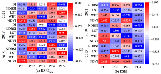
Figure 2.
Principal component analysis results of five factors for 2015, 2018, and 2021.
Table 3.
Principal component analysis of RSEInew and RSEI.
As shown in Figure 3, the average correlation between the RSEInew model and each factor was higher than that of RSEI. The average correlation between RSEInew and the five factors was 0.858, and that between RSEI and the four factors was 0.448. RSEInew and RSEI had consistent positive and negative correlations, respectively, for each factor. The correlation between the factors in the RSEInew model was stronger than in the RSEI model. The factor with the highest annual correlation between RSEInew and RSEI was NDBSI, indicating that NDBSI had the greatest impact on ecological environmental quality. This was mainly due to the decline in the ecological environment caused by the increase in urban expansion and construction land. Hence, compared with RSEI, RSEInew integrates the majority of the information of each factor, which is more representative than any single index and can better reflect the study area’s ecological environment.
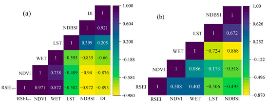
Figure 3.
Mean correlation of each indicator with (a) RSEInew and (b) RSEI.
3.2. Spatial and Temporal Pattern Analysis of RSEInew
3.2.1. Estimation of RSEInew
The annual mean value trends for the five ecological factors and RSEInew in UANSTM from 2015 to 2021 are shown in Figure 4. The overall annual average value of RSEInew demonstrated a decreasing trend, with a 3.12% rate of decline. The different years initially showed an increasing trend, followed by a decreasing trend. RSEInew increased from 0.321 in 2015 to 0.350 in 2017 and decreased to 0.311 in 2021. Similar to RSEInew, the annual average WET decreased by 7.22%. The annual mean values of the LST, NDBSI, and DI increased by 5%, 33.6%, and 6.61%, respectively.
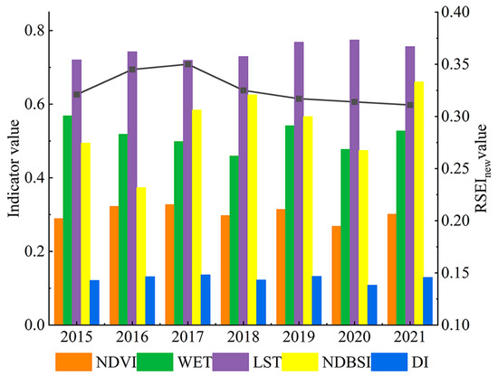
Figure 4.
The changes of the five indicators and RSEInew in UANSTM from 2015–2021.
3.2.2. Spatial Distribution Characteristics of RSEInew
As shown in Figure 5, the area with “strongly bad” ecological environmental quality increased by 8% in 2021 to approximately 6808.71 km2. The area with “slightly bad” ecological environmental quality decreased by 2.17% to approximately 1668.94 km2. The area with “neutral” ecological environmental quality decreased by 4.2%, and that with “slightly good” and “strongly good” ecological environmental quality decreased by approximately 1.61%. The grade transformation of RSEInew in the study area from 2015 to 2021 was mainly concentrated between “strongly bad” and “neutral.” Compared to other years, the RSEInew in 2017 was higher, indicating that the ecological environmental quality had improved dramatically.
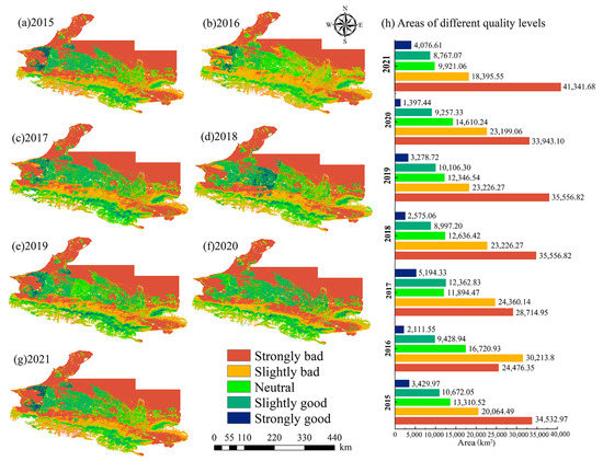
Figure 5.
Spatial distribution of RSEInew value classes in UANSTM.
To discover the dynamic characteristics of ecological environmental quality during different periods, the RSEInew of recent and previous years in the study area were subtracted to obtain the spatial difference (Figure 6). Figure 6 shows that the RSEInew in 2017 improved more than in 2015. Compared with 2017 and 2021, RSEInew showed a decreasing trend in 2019, and the deterioration area accounted for 17.77% and 9.13% of the total study area, respectively. Compared with 2015, the RSEInew deterioration area in 2021 was larger than the improved area, with the deterioration and improved areas accounting for 17.37% and 6.32% of the total area, respectively. Therefore, areas with degraded ecological quality are mainly located in the central cities, surrounding cities, and southern high-altitude areas. Areas where the quality of the ecological environment remained unchanged were mainly located in the northern desert and high-altitude forested areas. Areas with improved ecological quality were mainly located in central and western farmland. Areas of strong improvement and serious decline were very small, accounting for less than 1% of the total area, and areas with stable ecological environmental quality accounted for approximately 75% of the total area.
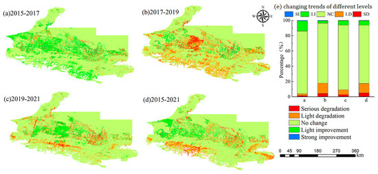
Figure 6.
RSEInew change in UANSTM from 2015 to 2021.
3.2.3. Seasonal Analysis of RSEInew
In this study, RSEInew was calculated for the spring (March, April, and May), summer (June, July, and August), and autumn (September, October, and November) seasons during different years in the study area based on the GEE platform. As shown in Table 4, the mean RSEInew values during spring from 2015 to 2021 presented decreasing, increasing, decreasing, increasing, and decreasing trends, respectively. An increasing-decreasing-increasing-decreasing trend was observed for the mean summer RSEInew values from 2015 to 2021. The mean fall RSEInew from 2015 to 2021 presented an increasing-decreasing-increasing-decreasing trend. These results show that RSEInew changes with time and environment, and the RSEInew estimated by selecting the remote sensing data of the same season or a certain day cannot accurately reflect the change characteristics of the ecological environmental quality for different years. Therefore, this study used high-quality Landsat remote sensing images in the spring, summer, and autumn of 2015–2021 (March–November) to construct the annual-scale RSEInew.
Table 4.
Changes in average seasonal RSEInew of the study area.
3.3. Coupling Relationship between Urbanization and Eco-Environment
3.3.1. Change in the Mean RSEInew Value in the Main City of UANSTM
From 2015 to 2021, the annual average RSEInew changes in the main urban areas of the nine major cities (Figure 7) showed that the ecological environmental quality of different cities in the study area was significantly different. From 2015 to 2021, the average RSEInew values of Urumqi City, Fukang City, Kelamayi City, and Hutubi County showed a decreasing trend, and the ecological environmental quality of Urumqi City and Kelamayi City was relatively poor. The RSEInew of Urumqi City decreased from 0.331 in 2015 to 0.278 in 2021. The RSEInew in Kelamayi City decreased from 0.239 in 2015 to 0.210 in 2021. The mean RSEInew values for Kuitun City, Shihezi City, Changji City, Shawan County, and Manasi County showed an increasing trend. The RSEInew of Manasi County increased from 0.535 in 2015 to 0.564 in 2021, and the RSEInew of Shawan County increased from 0.476 in 2015 to 0.578 in 2021. Compared with 2015, the average RSEInew value of Shawan County in 2021 exhibited the highest change, with an increase of 0.102, and the average RSEInew value of Shihezi City was the least changed, with an increase of 0.01.
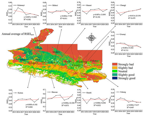
Figure 7.
The spatial distribution of average RSEInew in the study area and the change of average annual RSEInew in nine major cities from 2015 to 2021.
3.3.2. Extraction of Urbanization Features in UANSTM
Figure 8a–c shows the NTL space distribution in the study area for 2015 and 2020. The total number of pixels with light information and the brightness value in the study area exhibited an increasing trend. Among them, night lights were mainly concentrated in the three major urban agglomerations of the UANSTM: Urumqi-Fukang-Changji, Manasi-Shihezi-Shawan, and Kelamayi-Kuitun-Wusu. The lighted area increased from 3800.41 km2 in 2015 to 5785.42 km2 in 2020. In this study, the DN value of a light image was divided into four levels: very low, low, high, and very high [63]. Figure 8c,d shows that the areas with high DN values in 2020 relative to 2015 increased slightly, and areas with lower DN values increased significantly. It also indicates an increasing characteristic from the periphery to the center of the main urban area of the city and a contiguous distribution with neighboring cities.
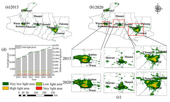
Figure 8.
Light images and their changes from 2015 to 2020 in the UANSTM.
Owing to the large area covered by this study, the non-construction land area is much greater than the construction land area. To avoid underestimating the urbanization level caused by the calculation of the CNLI of the municipal area, this study used the CNLI of the main urban areas of each city to investigate the urbanization level of the study area [64]. Table 5 shows that the MLI of major cities in the study area did not significantly change in 2015 and 2020, but the LAP and CNLI increased considerably. The LAP of the main urban areas of Manasi County, Kelamayi City, Kuitun City, and Changji City in 2020 increased by 27.9%, 27.1%, 25.3%, and 23.5%, respectively, compared with 2015, and the LAP of other cities increased by more than 10%. Based on these results, the urbanization levels of Urumqi City, Kelamayi City, Changji City, and Shihezi City were relatively high among the nine cities. In addition, cities with lower urbanization levels developed faster than those with higher urbanization levels. This shows that the urbanization development level of each city in UANSTM exhibits a rapid growth trend.
Table 5.
Mean change of mean light intensity (MLI), light area ratio product (LAP), and compounded nighttime light index (CNLI) in nine major cities of urban agglomeration on the northern slope of the Tianshan Mountains.
3.3.3. Coupling Coordination Degree Analysis of Different Cities
The coupling coordination degree was calculated based on the CCDM for the main urban areas of the major cities in the study area. Figure 9a,b shows that the coupling coordination degree of urbanization and ecological environmental quality in the main urban areas of the nine major cities from 2015 to 2020 exhibited an increasing trend, with an average increase from 0.221 in 2015 to 0.239 in 2020. Among them, the coupling coordination degree of Urumqi City, Changji City, Shihezi City, Kuitun City, and Kelamayi City was higher than that of the other cities. This indicates that the coupled coordinated development of urbanization and ecological environment has improved from 2015 to 2020; however, it is still characterized by moderate imbalance and a level of gradual urbanization. Therefore, although the urbanization and ecological environment of cities in UANSTM are changing rapidly, the coupling coordination between the two remains at a low level. Moreover, ecological environmental quality is changing at a faster rate than the development of urbanization and they have not reached the stage of coordinated development.
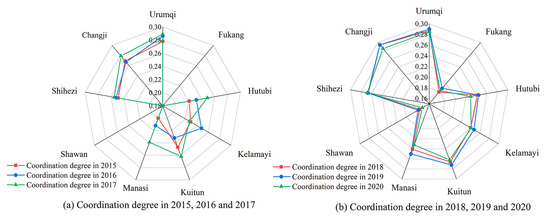
Figure 9.
Coupling and coordination of urbanization and ecological environmental quality in major cities of UANSTM.
4. Discussion
4.1. Suitability of RSEInew
With the rapid economic development and urban expansion in Xinjiang, air pollution has become an urgent environmental problem. The desert area is widely distributed, and the heating period is long in winter, resulting in PM2.5, which is the main air pollutant in Xinjiang. Particulate matter pollution poses a serious threat to human health and the ecological environment [65]. RSEInew, which comprehensively considers PM2.5, can more accurately evaluate the ecological environmental quality of the study area [66]. Through comparison and analysis, this paper finds that, compared with the general RSEI, this RSEInew is more effective in evaluating the ecological environment quality of urban clusters in arid zones, and this index can be more widely applied to the evaluation of ecological environment quality in arid zones in the future. Furthermore, this study used the GEE platform to estimate RSEInew with higher spatial and temporal resolution over a large area, which overcomes the problem of low accuracy of the estimation results because of the lack of remote sensing data, cloudiness, and time inconsistency in the traditional method of RSEI. The spatial and temporal characteristics of ecological environmental quality were extracted at monthly, seasonal, and annual intervals.
4.2. Cause Analysis of RSEInew Index and Coupling Coordination Degree
The results of the ecological environmental quality of UANSTM from 2015 to 2020 initially demonstrated a rising and then declining trend, where the quality of the ecological environment in 2017 was the best. Figure 4 shows that compared to other years, NDVI was positively correlated with the quality of the ecological environment, and LST was negatively correlated with the maximum and minimum values in 2017. We superimposed the effects of other factors to prove the best ecological quality performance in the study area in 2017. As approximately 45% of the land-use types in UANSTM are bare land with extremely low vegetation coverage [67], the overall ecological environmental quality is poor. Areas where the quality of the ecological environment has remained poor are the desert areas to the north. Areas with good ecological environmental quality were mainly concentrated in the central oasis agricultural area and southern pre-mountain grassland zone of the study area. The ecological quality of the study area strongly depends on water resources. Furthermore, with the continuous increase in urban construction land, the fragmentation of the vegetation landscape in the main urban area of the city and its surrounding areas has intensified and deteriorated the ecological environmental quality.
Figure 8 shows that the light intensity in the central areas of the cities with high urbanization levels (Urumqi City, Kelamyi City, Shihezi City, and Changji City) did not change significantly from 2015 to 2020, whereas the light intensity in the areas around the main urban areas increased significantly. The main reason is that the urbanization of the central urban area had a high level of urbanization in the early stage of this study; therefore, the light intensity changed less compared to the surrounding areas. From 2015 to 2020, the degree of coordinated development of urbanization and the ecological environment in the UANSTM showed an upward trend, but the overall condition was in a state of moderate imbalance, mainly due to gradual urbanization. From 2015 to 2020, the research area was in an important stage of accelerating economic development during the national “12th Five-Year Plan” and “13th Five-Year Plan” and promoting the sustainable and healthy development of the regional social economy. Motivated by relevant policies, UANSTM has achieved tremendous economic, social, and environmental development and progress. However, as the study area is underdeveloped in western China, urbanization development is relatively slow, and the fragile natural ecological environment is easily threatened by economic development. For cities with rapid urbanization and insufficient environmental input, the quality of the ecological environment declines with the acceleration of urbanization, resulting in a low overall degree of coupling and coordination between urbanization and the ecological environment in the study area. To improve the coordinated development of urbanization and the ecological environment in the study area, the primary task is to increase the pace of urban economic development and increase investment in environmental construction.
5. Conclusions
This study constructed RSEInew for the study area using the GEE platform. The remote sensing data of NTL were combined to estimate the index of the CNLI and comprehensively evaluate the coupling relationship between urbanization and ecological environmental quality in UANSTM and the main urban areas of major cities from 2015 to 2020. The main conclusions are as follows:
(1) From 2015 to 2021, the average RSEInew value of UANSTM ecological environmental quality improved and then deteriorated, with an overall declining trend. The quality changes for RSEInew were mainly concentrated between the “strongly bad” and “neutral” grades. The ecological quality of the study area showed strong dependence on water resources. In addition, with the continuous increase in urban construction land, vegetation landscape fragmentation in the main urban area and its surrounding areas is aggravated, and ecological environmental quality is decreased. RSEInew is more suitable for evaluating the quality of urban ecological environments in arid regions;
(2) From 2015 to 2020, the urbanization development level of the main urban areas in all cities exhibited an increasing trend. The degree of coupling coordination between urbanization and ecological environmental quality in the main urban areas of each city increased steadily each year; however, the coupling coordination remains at a low level;
(3) Approximately 45% of the land-use types in UANSTM were bare land, resulting in poor ecological environmental quality in the study area. Areas with good ecological environmental quality were mainly concentrated in the central oasis farming area and southern piedmont grassland zone. With the development and expansion of UANSTM, fragile ecological environments are under greater pressure. In the majority of the study area, the urbanization process is fast; however, environmental investment is insufficient, leading to the acceleration of urbanization but a decline in ecological environmental quality. Overall, this results in a low degree of coupling coordination between urbanization and the ecological environment. Therefore, to ensure the sustainability of environmental resources, urban development and environmental governance are equally important in arid areas. This study only discussed the impact of land-use type on ecological environmental quality. Future research should aim to analyze the impact of natural and human factors on eco-environmental quality, urbanization, and their degree of coordination.
Author Contributions
Conceptualization, M.Z. and P.H.; data curation, P.H.; formal analysis, P.H.; funding acquisition, M.Z.; methodology, P.H. and M.Z.; writing—original draft, P.H.; writing—review and editing, M.Z. All authors have read and agreed to the published version of the manuscript.
Funding
This research was funded by the Xinjiang Normal University Doctoral Research Start-up Fund Project (XJNUBS2003), and the Xinjiang Uygur Autonomous Region Key Laboratory Bidding Project (XJDX0909-2021-01).
Institutional Review Board Statement
Not applicable.
Informed Consent Statement
Not applicable.
Data Availability Statement
The data are available upon request by contact with the corresponding author.
Acknowledgments
We thank the three anonymous reviewers for their constructive comments and suggestions that have helped to improve the original manuscript. Thanks also to the editorial staff.
Conflicts of Interest
The authors declare no competing interests.
References
- Padhee, S.K.; Dutta, S. Spatio-temporal reconstruction of MODIS NDVI by regional land surface phenology and harmonic analysis of time-series. GISci. Remote Sens. 2019, 56, 1261–1288. [Google Scholar] [CrossRef]
- Chen, J.; Gao, J.; Chen, W. Urban land expansion and the transitional mechanisms in Nanjing, China. Habitat Int. 2016, 53, 274–283. [Google Scholar] [CrossRef]
- Sowińska-Świerkosz, B. Application of surrogate measures of ecological quality assessment: The introduction of the Indicator of Ecological Landscape Quality (IELQ). Ecol. Indic. 2017, 73, 224–234. [Google Scholar] [CrossRef]
- Luo, Y.; Sun, W.; Yang, K.; Zhao, L. China urbanization process induced vegetation degradation and improvement in recent 20 years. Cities 2021, 114, 103207. [Google Scholar] [CrossRef]
- Wang, S.; Ma, H.; Zhao, Y. Exploring the relationship between urbanization and the eco-environment-a case study of Beijing-Tianjin-Hebei region. Ecol. Indic. 2014, 45, 171–183. [Google Scholar] [CrossRef]
- Lee, L.S.H.; Zhang, H.; Jim, C.Y. Serviceable tree volume: An alternative tool to assess ecosystem services provided by ornamental trees in urban forests. Urban For. Urban Green. 2021, 59, 127003. [Google Scholar] [CrossRef]
- Qureshi, S.; Alavipanah, S.K.; Konyushkova, M.; Mijani, N.; Fathololomi, S.; Firozjaei, M.K.; Homaee, M.; Hamzeh, S.; Kakroodi, A.A. A remotely sensed assessment of surface ecological change over the Gomishan Wetland, Iran. Remote Sens. 2020, 12, 2989. [Google Scholar] [CrossRef]
- Tang, P.; Huang, J.; Zhou, H.; Fang, C.; Zhan, Y.; Huang, W. Local and telecoupling coordination degree model of urbanization and the eco-environment based on RS and GIS: A case study in the Wuhan urban agglomeration. Sustain. Cities Soc. 2021, 75, 103405. [Google Scholar] [CrossRef]
- Hazbavi, Z.; Sadeghi, S.H.; Gholamalifard, M.; Davudirad, A.A. Watershed health assessment using the pressure–state–response (PSR) framework. Land Degrad. Dev. 2020, 31, 3–19. [Google Scholar] [CrossRef]
- Novoa, J.; Chokmani, K.; Lhissou, R. A novel index for assessment of riparian strip efficiency in agricultural landscapes using high spatial resolution satellite imagery. Sci. Total Environ. 2018, 644, 1439–1451. [Google Scholar] [CrossRef]
- Tang, W.; Zhou, T.; Sun, J.; Li, W. Accelerated urban expansion in lhasa city and the implications for sustainable development in a Plateau City. Sustainability 2017, 9, 1499. [Google Scholar] [CrossRef]
- Ochoa-Gaona, S.; Kampichler, C.; De Jong, B.H.J.; Hernández, S.; Geissen, V.; Huerta, E. A multi-criterion index for the evaluation of local tropical forest conditions in Mexico. For. Ecol. Manag. 2010, 260, 618–627. [Google Scholar] [CrossRef]
- Zhang, R.G.; Mo, X.G.; Liu, Z.H. The trend and principal influence factors of evapotranspiration in Hutuo River Basin during last 50 years. Sci. Geogr. Sin. 2012, 32, 628–634. [Google Scholar]
- Cui, Q.Y.; Pan, Y.; Yang, X. Beijing plain area of remote sensing images based on Landsat 8 impermeable layer coverage estimates. J. Cap. Norm. Univ. (Nat. Sci. Ed.) 2015, 36, 89–92. [Google Scholar]
- Xu, H.Q. A remote sensing urban ecological index and its application. Acta Ecol. Sin. 2013, 33, 7853–7862. [Google Scholar]
- Liao, W.; Jiang, W. Evaluation of the spatiotemporal variations in the eco-environmental quality in China based on the remote sensing ecological index. Remote Sens. 2020, 12, 2462. [Google Scholar] [CrossRef]
- Huang, H.; Chen, W.; Zhang, Y.; Qiao, L.; Du, Y. Analysis of ecological quality in Lhasa Metropolitan Area during 1990–2017 based on remote sensing and Google Earth Engine platform. J. Geogr. Sci. 2021, 31, 265–280. [Google Scholar] [CrossRef]
- Zhu, D.Y.; Chen, T.; Niu, R.Q.; Zhen, N. Analyzing the ecological environment of mining area by using moving window remote sensing ecological index. Wuhan Daxue Xuebao Xinxi Kexueban 2021, 46, 341–347. [Google Scholar]
- Wang, S.D.; Si, J.J.; Wang, Y. Study on Evaluation of Ecological Environment Quality and Temporal-Spatial Evolution of Danjiang River Basin (Henan Section). Pol. J. Environ. Stud. 2021, 30, 2353–2367. [Google Scholar] [CrossRef]
- Stirnberg, R.; Cermak, J.; Andersen, H. An analysis of factors influencing the relationship between satellite-derived AOD and ground-level PM10. Remote Sens. 2018, 10, 1353. [Google Scholar] [CrossRef]
- Yao, L.; Li, X.; Li, Q.; Wang, J. Temporal and spatial changes in coupling and coordinating degree of new urbanization and ecological-environmental stress in China. Sustainability 2019, 11, 1171. [Google Scholar] [CrossRef]
- Cai, B.; Shao, Z.F.; Fang, S.H.; Huang, X.; Huq, M.E.; Tang, Y.; Li, Y.; Zhuang, Q. Finer-scale spatiotemporal coupling coordination model between socioeconomic activity and eco-environment: A case study of Beijing, China. Ecol. Indic. 2021, 131, 108165. [Google Scholar] [CrossRef]
- Chen, X.H.; Zhou, H.H. Research hotspots and prospects of urbanization and ecological environment relationship based on visual knowledge mapping. Prog. Geogr. 2018, 37, 1171–1185. [Google Scholar]
- Fang, N.; Zhang, Q.; Yang, D.X. Spatial-temporal evolution and coupling coordination between ecological civilization construction and urbanization in Hunan Province. Areal Res. Dev. 2020, 39, 59–64. [Google Scholar]
- Liang, L.W.; Wang, Z.B.; Fang, C.L.; Sun, Z. Spatiotemporal differentiation and coordinated development pattern of urbanization and the ecological environment of the Beijing-Tianjin-Hebei urban agglomeration. Acta Ecol. Sin. 2019, 39, 1212–1225. [Google Scholar]
- Chu, N.C.; Wu, X.L.; Zhang, P.Y.; Li, H.; Yang, Q.F. Spatiotemporal evolution characteristics of coordinated development of urbanization and ecological environment in eastern Russia. Acta Ecol. Sin. 2021, 41, 9717–9728. [Google Scholar]
- Tao, C.J.; Xia, A.T.; Li, D.P. Research on the coupling coordination development of urbanization and ecological environment in Maanshan City. Ecol. Sci. 2021, 40, 129–138. [Google Scholar]
- Zhang, L.F.; Fang, C.L.; Gao, Q. Spatial and temporal expansion of urban landscape and multi-scene simulation of urban agglomeration in northern slope of Tianshan Mountains. Acta Ecol. Sin. 2021, 41, 1267–1279. [Google Scholar]
- Fang, C.L. Strategic thinking and spatial layout for the sustainable development of urban agglomeration in northern slope of Tianshan Mountains. Arid Land Geogr. 2019, 42, 1–11. [Google Scholar]
- Xu, H. A new index for delineating built-up land features in satellite imagery. Int. J. Remote Sens. 2008, 29, 4269–4276. [Google Scholar] [CrossRef]
- Zha, Y.; Gao, J.; Jiang, J.; Lu, H.; Huang, J. Normalized difference haze index: A new spectral index for monitoring urban air pollution. Int. J. Remote Sens. 2012, 33, 309–321. [Google Scholar] [CrossRef]
- Chen, Z.; Yu, B.L.; Yang, C.S.; Zhou, Y.Y.; Yao, S.J.; Qian, X.J.; Wang, C.X.; Wu, B.; Wu, J.P. An extended time series (2000–2018) of global NPP-VIIRS-like nighttime light data from a cross-sensor calibration. Earth Syst. Sci. Data 2021, 13, 889–906. [Google Scholar] [CrossRef]
- Wan, H.L.; Huo, F.; Niu, Y.; Zhang, W.; Zhang, Q. Dynamic monitoring and analysis of ecological environment change in Cangzhou city based on RSEI model considering PM2. 5 concentration. Prog. Geophys. 2021, 36, 953–960. [Google Scholar]
- Feng, H.Y.; Feng, Z.K.; Feng, H.X. One new method of PM2.5 concentration inversion based on difference index. Spectrosc. Spectr. Anal. 2018, 38, 3012. [Google Scholar]
- Feng, H.X.; Feng, H.Y.; Yang, L.C.; Wang, Q.; Meng, X.L.; Wang, Y.F. A remote sensing monitoring method of urban air quality based on Landsat 8. Huanjing Wuran Yu Fangzhi 2021, 43, 79–83+90. [Google Scholar]
- Yan, L.; He, R.; Kašanin-Grubin, M.; Luo, G.; Peng, H.; Qiu, J. The Dynamic Change of Vegetation Cover and Associated Driving Forces in Nanxiong Basin, China. Sustainability 2017, 9, 443. [Google Scholar] [CrossRef]
- Jin, S.; Sader, S.A. Comparison of time series tasseled cap wetness and the normalized difference moisture index in detecting forest disturbances. Remote Sens. Environ. 2005, 94, 364–372. [Google Scholar] [CrossRef]
- Baig, M.H.A.; Zhang, L.; Shuai, T.; Tong, Q. Derivation of a tasselled cap transformation based on Landsat 8 at-satellite reflectance. Remote Sens. Lett. 2014, 5, 423–431. [Google Scholar] [CrossRef]
- Xu, H. Assessment of ecological change in soil loss area using remote sensing technology. Trans. Chin. Soc. Agric. Eng. 2013, 29, 91–97. [Google Scholar]
- Liu, G.; Zhang, Q.; Li, G.; Doronzo, D.M. Response of land cover types to land surface temperature derived from Landsat-5 TM in Nanjing Metropolitan Region, China. Environ. Earth. Sci. 2016, 75, 1386. [Google Scholar] [CrossRef]
- Yu, X.; Guo, X.; Wu, Z. Land surface temperature retrieval from Landsat 8 TIRS—Comparison between radiative transfer equation-based method, split window algorithm and single channel method. Remote Sens. 2014, 6, 9829–9852. [Google Scholar] [CrossRef]
- Yang, J.; Duan, S.B.; Zhang, X.; Wu, P.; Huang, C.; Leng, P.; Gao, M. Evaluation of seven atmospheric profiles from reanalysis and satellite-derived products: Implication for single-channel land surface temperature retrieval. Remote Sens. 2020, 12, 791. [Google Scholar] [CrossRef]
- Gao, W.; Zhang, S.; Rao, X.; Lin, X.; Li, R. Landsat TM/OLI-Based Ecological and Environmental Quality Survey of Yellow River Basin, Inner Mongolia Section. Remote Sens. 2021, 13, 4477. [Google Scholar] [CrossRef]
- Hu, X.; Xu, H. A new remote sensing index for assessing the spatial heterogeneity in urban ecological quality: A case from Fuzhou City, China. Ecol. Indic. 2018, 89, 11–21. [Google Scholar] [CrossRef]
- Rikimaru, A.; Roy, P.S.; Miyatake, S. Tropical forest cover density mapping. Trop. Ecol. 2002, 4, 39–47. [Google Scholar]
- Essa, W.; Verbeiren, B.; van der Kwast, J.; Van de Voorde, T.; Batelaan, O. Evaluation of the DisTrad thermal sharpening methodology for urban areas. Int. J. Appl. Earth Obs. 2012, 19, 163–172. [Google Scholar] [CrossRef]
- Awad, M.; Aldaood, A.; Alkiki, I. Development of a Compressibility Prediction Model Based on Soil Index Properties and Area Under/Bounded by Consolidation and Rebound Curves. Geotech. Geol. Eng. 2022, 40, 4787–4807. [Google Scholar] [CrossRef]
- Wang, Y.H.; Xiao, Y. Inversion and Spatial-temporal distribution analysis on PM5.0 inhalable particulate in Beijing. Environ. Sci. 2014, 35, 428–435. [Google Scholar]
- He, J.L.; Zhang, S.Y.; Li, J.; Zha, Y. Particulate matter indices derived from MODIS data for dictating urban air pollution. Remote Sens. Land Resour. 2016, 28, 126–131. [Google Scholar]
- Xu, H.; Wang, M.; Shi, T.; Guan, H.; Fang, C.; Lin, Z. Prediction of ecological effects of potential population and impervious surface increases using a remote sensing based ecological index (RSEI). Ecol. Indic. 2018, 93, 730–740. [Google Scholar] [CrossRef]
- Wang, B.; Chen, L.; Li, L.; Xie, H.; Zhang, Y. Ecological response to land use change: A case study from the Chaohu lake basin, China. Bulg. Chem. Commun. 2017, 49, 200–206. [Google Scholar]
- Boori, M.S.; Choudhary, K.; Paringer, R.; Kupriyanov, A. Spatiotemporal ecological vulnerability analysis with statistical correlation based on satellite remote sensing in Samara, Russia. J. Environ. Manag. 2021, 285, 112138. [Google Scholar] [CrossRef] [PubMed]
- Yuan, B.D.; Fu, L.; Zou, Y.A.; Zhang, S.Q.; Chen, X.S.; Li, F.; Deng, Z.M.; Xie, Y.H. Spatiotemporal change detection of ecological quality and the associated affecting factors in Dongting Lake Basin, based on RSEI. J. Clean. Prod. 2021, 302, 126995. [Google Scholar] [CrossRef]
- Zhang, T.; Yang, R.; Yang, Y.; Li, L.; Chen, L. Assessing the Urban Eco-Environmental Quality by the Remote-Sensing Ecological Index: Application to Tianjin, North China. ISPRS Int. J. Geo-Inf. 2021, 10, 475. [Google Scholar] [CrossRef]
- Zheng, Z.H.; Wu, Z.; Chen, Y.B.; Yang, Z.W.; Marinello, F. Analyzing the ecological environment and urbanization characteristics of the Yangtze River Delta Urban Agglomeration based on Google Earth Engine. Acta Ecol. Sin. 2021, 41, 717–729. [Google Scholar]
- Zhuo, L.; Shi, P.; Chen, J. Application of compound night light index derived from DMSP/OLS data to urbanization analysis in China in the 1990s. Acta Geogr. Sin. 2003, 58, 893–902. [Google Scholar]
- Liu, W.; Jiao, F.; Ren, L.; Xu, X.; Wang, J.; Wang, X. Coupling coordination relationship between urbanization and atmospheric environment security in Jinan City. J. Clean. Prod. 2018, 204, 1–11. [Google Scholar] [CrossRef]
- Liu, H.; Huang, B.; Yang, C. Assessing the coordination between economic growth and urban climate change in China from 2000 to 2015. Sci. Total Environ. 2020, 732, 139283. [Google Scholar] [CrossRef]
- Shen, L.; Huang, Y.; Huang, Z.; Lou, Y.; Ye, G.; Wong, S.W. Improved coupling analysis on the coordination between socio-economy and carbon emission. Ecol. Indic. 2018, 94, 357–366. [Google Scholar] [CrossRef]
- Hui, D.Y.; Guo, X. The measurement of the coordinated development level of economy resources environment in western regions. Stat. Decis. 2019, 11, 124–128. [Google Scholar]
- Ruili, G.; Linlin, W. Evaluation of Coordinated Development of Urbanization and Ecological Environment in the Efficient Ecological Economic Zone of the Yellow River Delta. Meteorol. Environ. Res. 2018, 9, 47–51. [Google Scholar]
- Ariken, M.; Zhang, F.; Liu, K.; Fang, C.; Kung, H.T. Coupling coordination analysis of urbanization and eco-environment in Yanqi Basin based on multi-source remote sensing data. Ecol. Indic. 2020, 114, 106331. [Google Scholar] [CrossRef]
- Zheng, Z.; Wu, Z.; Chen, Y.; Yang, Z.; Marinello, F. Exploration of eco-environment and urbanization changes in coastal zones: A case study in China over the past 20 years. Ecol. Indic. 2020, 119, 106847. [Google Scholar] [CrossRef]
- Meng, D.; Liu, L.; Gong, H.; Li, X.; Jiang, B. Coupling and coordination relationships between urbanization and ecological environment along the Beijing-Hangzhou Grand Canal. Remote Sens. Land Resour. 2021, 33, 162–172. [Google Scholar]
- Yang, L. Estimating PM2.5 concentrations in eastern coastal area of China using a two-stage random forest model. Remote Sens. Land Resour. 2020, 32, 137–144. [Google Scholar]
- Wan, H.L.; Wang, F.C.; Zhang, W.; Bao, Y.L.; Zhang, L.J.; Zhang, H.; Li, Q. Analysis of land use change driven by the construction of the Grand Canal cultural belt and its ecological effects: Taking Cangzhou section as a case. Prog. Geophys. 2022, 37, 1863–1874. [Google Scholar]
- Chen, Y.; Cheng, X.; Wang, J.L. Analysis of temporal and spatial dynamic changes of farmland in north slope economic zone of Tianshan Mountain from 1990 to 2020. J. Shihezi Univ. (Nat. Sci.) 2022, 40, 223–230. [Google Scholar]
Disclaimer/Publisher’s Note: The statements, opinions and data contained in all publications are solely those of the individual author(s) and contributor(s) and not of MDPI and/or the editor(s). MDPI and/or the editor(s) disclaim responsibility for any injury to people or property resulting from any ideas, methods, instructions or products referred to in the content. |
© 2023 by the authors. Licensee MDPI, Basel, Switzerland. This article is an open access article distributed under the terms and conditions of the Creative Commons Attribution (CC BY) license (https://creativecommons.org/licenses/by/4.0/).