Article

Exploring Primary Aluminum Consumption: New Perspectives from Hybrid CEEMDAN-S-Curve Model

1
Institute of Mineral Resources, Chinese Academy of Geological Sciences, Beijing 100037, China
2
Qinghai Salt Lake Industry Co., Ltd., Golmud 816000, China
*
Author to whom correspondence should be addressed.
Sustainability 2023, 15(5), 4228; https://doi.org/10.3390/su15054228
Submission received: 17 September 2022 / Revised: 17 February 2023 / Accepted: 23 February 2023 / Published: 26 February 2023
(This article belongs to the Section Sustainable Materials)

Abstract

:
Aluminum is globally the most used nonferrous metal. Clarifying the consumption of primary aluminum is vital to economic development and emission reduction. Based on the signal decomposition tool and S-curve model, a new hybrid complete ensemble empirical mode decomposition with adaptive noise (CEEMDAN)-S-curve model is proposed to analyze primary aluminum consumption of different countries for the last 100 years. The results show that: (1) Per capita primary aluminum consumption can be decomposed into low-frequency, medium-frequency, and high-frequency components, contributing over 70%, 2–17%, and less than 9% to variability of consumption series, respectively. This can be interpreted as economic development represented by GDP per capita, shocks from significant events, and short-term fluctuations, respectively. (2) The CEEMDAN-S-curve shows good applicability and generalizability by using this model in different countries. (3) A new strategy is provided to analyze and predict the consumption pattern of primary aluminum. Furthermore, some important topics related to primary aluminum consumption are discussed, such as CO2 emission and recovery. Based on the results, to meet economic development and achieve sustainable development goals, some measures should be implemented, such as making policies, encouraging resource recovery, and developing new technologies.

1. Introduction

Aluminum (Al), a chemical element, is a lightweight silvery white metal of main Group 13 (IIIa, or boron group) of the periodic table. Aluminum is the most abundant metallic element in Earth’s crust and the most widely used nonferrous metal. Because of its chemical activity, aluminum never occurs in the metallic form in nature, but its compounds are present to a greater or lesser extent in almost all rocks, vegetation, and animals [1]. Aluminum occurs in igneous rocks chiefly as aluminosilicates in feldspars, feldspathoids, and micas; in the soil derived from them as clay; and upon further weathering as bauxite and iron-rich laterite [2].
Due to excellent mechanical properties, low density, high corrosion resistance, and easy recovery, aluminum and aluminum alloys are widely used in many fields, such as transportation, building structures, power electronics, packaging containers, durable consumer products, and machinery manufacturing. As one of the important bulk commodities, the consumption of global primary aluminum has been increasing since the 1920s, and this trend is projected to continue for a long time (Figure 1) [2]. In 2020, global primary aluminum consumption was more than 9 500 times higher than in 1920, reaching 65 million tons. The major consumption countries are China, India, Japan, and the United States [3].
However, aluminum production is an energy-intensive industry. The amount of greenhouse gas (GHG) emitted per ton of aluminum produced is seven to nine times more than that emitted per ton of steel [2]. In the full life cycle (cradle-to-gate) of aluminum, primary aluminum is the major GHG emission sector, accounting for 90% (Figure S1) [3]. In addition, aluminum price has been fluctuating sharply, which has affected the average profit of the aluminum industry (Figure S2) [4]. The continuous growth in primary aluminum consumption has brought about challenges to the industry, including energy consumption and environmental pollution. As a result, clarifying the consumption pattern of primary aluminum is not only important for economic development, but also necessary for sustainable development.

1.1. Literature Review

Many scholars and institutions have studied aluminum consumption and achieved fruitful results [5,6,7,8]. These studies mainly focus on demand forecasting, consumption and carbon emissions, consumption and resource recovery, and consumption and energy. For example, Yi et al. [5] analyzed global carbon emissions and transfers from aluminum production, consumption, and trade from 2000 to 2018, then revealed the carbon distribution across regions and countries. Monica et al. [9] analyzed the consumption status of aluminum resources in India, and used the MARKAL model to predict the energy demand of the aluminum industry from 2010 to 2031. Li et al. [10] used dynamic material flow analysis (MFA), regression analysis, and normal life distribution to estimate the domestic consumption, scrap generation, and in-use stock of aluminum from 1990 to 2030 in China. Du et al. [11] used life cycle assessment methodology to evaluate the impact of aluminum-intensive vehicles on GHG emissions and energy consumption.
Despite the extensive research on aluminum consumption, the consumption mechanism of primary aluminum has not been thoroughly studied. This is due to the nonlinearity and randomness of consumption series, as well as the utilization of different application methods, which result in different research outcomes [12,13,14].
The most common analysis method of primary aluminum consumption pattern is econometric analysis, which uses regression analysis, economic structure models, and other models to establish the relationship between the consumption and socio-economic indicators such as GDP, population, or per capita GDP [15,16,17,18,19]. Material flow analysis (MFA) has also been used to analyze primary consumption [20,21,22,23]. This method reveals the aluminum material flow characteristics from each link in the aluminum industry and provides the basis for an analysis framework of the entire aluminum material flow life cycle [1,24,25].
Furthermore, in order to accurately capture data characteristics, more scholars and institutions are beginning to explore non-standard or algorithmic models to explain the primary aluminum consumption mechanism, such as artificial neural networks (ANN), support vector machine (SVM), genetic algorithm (GA), gray model (GM), and empirical mode decomposition (EMD) [26,27,28]. Xu et al. [29] used the GA method and regression algorithms to predict primary aluminum consumption in China. Yuan et al. [30] used the ANN model to dynamically analyze China’s primary aluminum consumption and its influencing factors. It is concluded that China’s demand for aluminum resources occurred under three different scenarios from 2014 to 2020.
However, these single methods still have limitations in expressing the nonlinear characteristics of the data, quantifying the impact factors of consumption patterns, and improving the accuracy of the results. Therefore, there has been a growing interest in using hybrid models to overcome the limitations of individual models. [31]. Using hybrid models allows researchers to leverage the strengths of different modeling techniques and overcome their limitations. As such, we can expect to see more innovative and integrated models to study primary aluminum consumption patterns in the future.

1.2. Research Gap

Previous studies have provided valuable insights into the primary aluminum consumption. However, there are still some research gaps that need to be addressed.
Firstly, most existing studies have focused on analyzing the current state and short-term trends of primary aluminum consumption, which has led to a lack of research on long-term trends and future predictions. Long-term trends and future predictions are essential for decision-making and planning, as they provide insights into the direction of primary aluminum consumption.
Secondly, many studies have been limited in their scope, with some focusing solely on specific countries or regions, without providing a comprehensive analysis of global aluminum consumption. A comprehensive analysis of global aluminum consumption is necessary to understand the factors that affect primary aluminum consumption on a global scale.
In addition, despite some studies using different modeling techniques, a unified and comprehensive framework that integrates the various factors influencing primary aluminum consumption is still lacking. Furthermore, existing methods for analyzing primary aluminum consumption have limitations, such as difficulty revealing the nonlinear characteristics of the data.
Therefore, there is a need for research to focus on the long-term trends and future predictions of primary aluminum consumption, alongside a more comprehensive analysis of global aluminum consumption. Additionally, a unified framework should be developed to integrate the various factors affecting primary aluminum consumption. Research methods must be continuously improved to reveal the nonlinear characteristics of the data, and multiple methods are recommended, such as GA-GM model, EMD-SVM model.

1.3. Theory and Purpose of This Study

Per capita primary aluminum consumption is a complex indicator that reflects the interplay of multiple economic, technological, and environmental factors, in addition to market dynamics and consumer behavior. Capturing the nonlinear and intricate features of such a series poses a challenge for researchers. To address this, this study introduces a novel hybrid model that combines the complete ensemble empirical mode decomposition with adaptive noise (CEEMDAN) and the S-curve model. By utilizing this model, the per capita primary aluminum consumption series is decomposed, reconstructed, and interpreted, thus providing a better understanding of the primary aluminum consumption mechanism.
CEEMDAN is a signal decomposition tool that decomposes a non-stationary time series into a finite number of intrinsic mode functions (IMFs) and a residue. It is an extension of the original EEMD (Empirical Mode Decomposition) algorithm and improves its performance by adding a white noise layer to the input data and adaptively adjusting the amplitude of the noise layer. By using this tool, the complex nonlinear data series can be decomposed into simpler and more meaningful components, making it easier to analyze the characteristics and patterns of the data [32,33].
The S-curve model is a mathematical model that describes the relationship between primary aluminum consumption and various influencing factors. The S-curve model assumes that per capita primary aluminum consumption starts with a slow-growing trend, transitions to a relatively fast-growing trend, then changes to a declining growth trend, and finally reaches a stagnant trend. The model quantifies the influence of different factors on the consumption process by using a formula that describes the relationship between the consumption and the factors. Then, this formula can also be used to predict the future consumption trend [34].
The combination of CEEMDAN and the S-curve model in the proposed hybrid model can overcome the limitations of using a single method to analyze primary aluminum consumption. By decomposing the nonlinear data series into simpler components with CEEMDAN, the hybrid model can accurately capture the features of the data and identify the patterns and trends of the consumption process. By using the S-curve model to quantify the influence of different factors on the consumption process, the hybrid model can provide a more comprehensive and accurate analysis of primary aluminum consumption and its driving factors. More details of the CEEMDAN–S-curve are shown in Section 2.
The purpose of this paper is to develop an effective hybrid CEEMDAN-S-curve method to explore the consumption mechanism of primary aluminum and quantify different influencing factors. This study focuses on the global consumption pattern of primary aluminum. The proposed hybrid model is expected to overcome the limitations of single models and provide a deeper understanding of the consumption mechanism of primary aluminum.

1.4. Novelty and Contributions

This study makes several notable contributions to the field of primary aluminum consumption research.
Firstly, the study is unique in its comprehensive and extensive data analysis, spanning a time frame of over 100 years and examining the primary aluminum consumption of nine representative countries. This extensive research approach allows for a thorough understanding of the long-term trends and patterns of primary aluminum consumption and provides a foundation for future research in this area.
Secondly, it presents a quantitative and direct analysis of the consumption mechanism of primary aluminum. By decomposing the primary aluminum consumption series using the CEEMDAN-S-curve model, this study is able to quantify the contribution of various driving factors to the volatility of the original series. Specifically, this analysis explains the impact of economic development, significant events, and normal market activities on primary aluminum consumption, providing valuable insights into the complex factors influencing primary aluminum consumption.
Finally, this study demonstrates the good stability and applicability of the CEEMDAN-S-curve model in the analysis of primary aluminum consumption. This model provides a clear and simple understanding of the data while also maintaining a high level of data logicality. Moreover, this model can be used to predict primary aluminum consumption, making it a valuable tool for demand forecasting.
The remainder of this paper is organized as follows. The materials and methods that are used in this study are briefly described in Section 2. Following that, in Section 3, the experimental results obtained from primary aluminum consumption datasets are presented. The consumption mechanism of primary aluminum is discussed in Section 4. Finally, the study is concluded in Section 5.

2. Materials and Methods

This section provides a detailed introduction to the CEEMDAN and S-curve models, including their development, applications, and usage. Based on these two methods, the CEEMDAN-S-curve model framework is constructed, and the application steps of the model are elaborated in detail. The data processing, analysis, and result statistics tools used in this study are mainly implemented through Matlab 2016b and Excel 2016.

2.1. Complete EnsembleEmpirical Mode Decomposition with Adaptive Noise

EMD is an adaptive signal processing technique introduced to analyze nonlinear and non-stationary time series. It consists of a local and fully data-driven separation of a time series in fast and slow oscillations [32]. The core of CEEMDAN is to decompose the data into a small number of independent and periodic intrinsic modes based on the local characteristic scale, which is defined as the distance between two successive local extreme values in EMD [33]. Therefore, the specific connotation of each mode can be analyzed based on a different scale.
However, EMD experiences some problems, such as the presence of oscillations of very disparate amplitude in a mode, or the presence of very similar oscillations in different modes, named mode mixing. To overcome these problems, EEMD method was proposed. EEMD features stronger self-adaptability and local variation characteristics, while effectively detecting the non-stationarity and nonlinearity [32]. It separates the embedded oscillations at different scales into intrinsic mode functions (IMFs) and a residual (trend) component.
Similarly, to avoid mode mixing problems and be self-adaptive, the CEEMDAN technique was proposed by Torres et al. [35]. With that, the reconstructed time series is identical to the intact (unresolved) one [36]. The key dissimilarity is that during the CEEMDAN decomposition process, a Gaussian white noise with unit variance and noise coefficient is added at each of the decomposition stages [37]. This noise-added signal is decomposed via EMD to obtain the first IMF and the subsequent residual component. Consider an unresolved signal, x(t), and added white noise, sn(t). To obtain the first IMF by CEEMDAN (i.e., IMF1), for every n = 1…, N decompose each x n (t) = x(t) + εsn(t) via EMD where: N = ensemble number and ε = amplitude of the added noise. More details of the CEEMDAN are shown in Supplementary Materials. Matlab 2016b code is available at: http://perso.ens-lyon.fr/patrick.flandrin/emd.html (accessed on 10 November 2022).

2.2. S-Curve Model

The S-curve pattern, first proposed by French mathematician Pierre-Francois Verhulst in 1838 for description of self-limiting growth of a biological population, has been employed to quantify the relationships of energy and mineral resource consumption and GDP per capita [38]. The S-curve pattern can be universally observed for most developed economies particularly since the twentieth century. Given that an economy has started from an increasing GDP stage, the energy and mineral resource consumption per capita starts with a low and slow growing trend, turns to a comparatively fast-growing trend, then changes to a declining growth trend, and finally reaches a stagnant trend [34,39]. There are three critical GDP points, take-off point, turning point, and zero-growth point, in S-curve patterns (Figure 2).
These thresholds mark important transformation periods of an economic structure:
(1)
Take-off point. This marks the second GDP growing phase at a high rate of energy and mineral resource consumption and the transition from agricultural society to industrial society.
(2)
Turning point. This marks declination in energy and mineral resources consumption rate per capita for a given GDP per capita.
(3)
Zero-growth point. This indicates a drastic change from growing to declining in the pattern of energy consumption per capita.
The mathematical technique is employed to describe the S-curve model to analyze and forecast future energy and mineral resource consumption. The relation of per capita primary aluminum consumption (Al) and per capita GDP (G) can be expressed as below (Equation (1)):
A l A l i = A e x p [ α 1 ( G G i ) ] e x p [ α 3 ( G G i ) ] 2 c o s h [ α 2 ( G G i ) ]
where α 1 , α 2 , α 3 are exponential constants, Gi and Ali are the GDP per capita value and per capita primary aluminum consumption, respectively, and A is the amplitude of the equation. Equation (1) is plotted as a hyperbolic tangent function.
Furthermore, the S-curve model summarizes the factors affecting energy and mineral resource consumption. These indicators can be divided into three categories: core indicators, constraint indicators, and reference indicators.
(1)
core indicators. Core indicators include economic and social indicators, and resource indicators. Economic and social indicators include GDP and population. GDP per capita, as a specific indicator, is the fundamental driving force for consumption. Resource indicators, including resource consumption growth rate, are important parameters to measure resource consumption.
(2)
constraint indicators. Constraint indicators refer to those indicators that have a close impact on resource consumption, such as resource consumption intensity, urbanization rate, industrial structure, resource policy, and price. It can reflect, measure, or constrain resource consumption from different aspects.
(3)
reference indicators. Reference indicators include infrastructure construction and social wealth accumulation, such as the number of bridges, ports, and airports, and social building areas. Although those indicators are difficult to directly relate to energy and mineral resource consumption, the level and trend of energy and resource consumption are determined by reference indicators.
The modeling process of the S-curve model is shown in Supplementary Materials.

2.3. CEEMDAN–S-Curve Model

The CEEMDAN–S-curve model is presented in Figure 3.
The CEEMDAN–S-curve model can be separated into six steps:
Step 1: Data processing.
The data used in this study are related to the production, consumption, trade volume (import and export volume), population, and other economic and social factors of the world. The consumption data are sourced from: (1) the direct use of apparent consumption; and (2) the equation of apparent consumption = domestic production + imports − exports − inventory.
Step 2: CEEMDAN decomposition.
Using CEEMDAN to decompose the consumption series into IMFs and a residue. Each IMF component represents the local characteristic time scale by itself. The results of this step are k IMFs (k is the number of IMFs) and a residue (Equation (2)):
Y t = [ I M F 1 , t I M F 2 , t I M F 3 , t I M F k , t R k , t ] = [ x 1 , 1 x 1 , 2 x 1 , 3 x 1 , N x 2 , 1 x 2 , 2 x 2 , 3 x 2 , N x 3 , 1 x 3 , 2 x 3 , 3 x 3 , N . . . x k , 1 x k , 2 x k , 3 x k , N x k + 1 , 1 x k + 1 , 2 x k + 1 , 3 x k + 1 , N ]
Step 3: Components reconstruction.
All component are reconstructed based on the Lempel–Ziv complexity values of each IMF to improve the reliability of the model. The Lempel–Ziv complexity values represent the periodicity, variability, and randomness of the components, where a higher value of the component indicates fewer periodic components, lower regularity of change, and more randomness [40]. The results of component reconstruction are low-frequency, medium-frequency, and high-frequency components.
Step 4: S-curve analysis.
The reconstructed components are analyzed and explained based on the S-curve model, taking into account the data characteristics of each component.
Step 5: Model test.
The reliability and stability of the CEEMDAN–S-curve are tested by selecting the test country and repeating the above steps.
Step 6: Results output.
The analysis results of primary aluminum consumption are summarized and presented.

3. Results

3.1. Data Processing

Aluminum production technology was not fully developed until the 1940s, which explains why the widespread application of aluminum began later than that of copper and iron. As shown in Figure 4, the consumption of primary aluminum has increased rapidly over the past century, particularly after the 1940s, which is in line with the development of aluminum production technology. It also reveals that primary aluminum consumption varies significantly among different countries, reflecting differences in their economic and industrial development levels.
Moreover, the relationship between primary aluminum consumption and other related indicators is analyzed (Figure S3). The results show that primary aluminum consumption shows regularity. Examples are the S-curve between the per capita primary aluminum consumption and GDP per capita in different countries, and the inverted U-shaped between the intensity of primary aluminum consumption and GDP per capita.

3.2. CEEMDANDecomposition

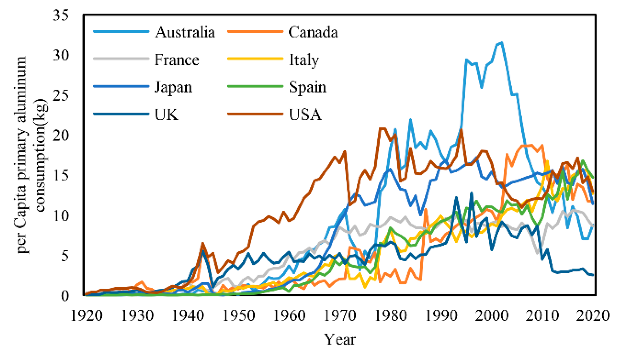
Different countries as samples may affect the generalizability of the findings. Australia, Canada, France, Italy, Japan, Spain, the United States, and the United Kingdom are major players in the global aluminum industry and have a long history of primary aluminum consumption. As such, they provide a useful benchmark for understanding the relationship between primary aluminum consumption and other related indicators (Figure 5 and Figure S3). The S-curve pattern is observed in the per capita primary aluminum consumption in these countries. These findings may be useful for policymakers in developing countries who are looking to promote sustainable economic growth and reduce greenhouse gas emissions. The series decomposition results are shown in Figure S4 and Table S1.
The following measures are taken to analyze IMFs: mean period of each IMF, Lempel–Ziv complexity, correlation between each IMF and the original data series, the variance and variance percentage of each IMF.
The mean period here is defined as the value derived by dividing the total number of points by the number of peaks for each IMF, since the frequency and the amplitude of an IMF may change with time continuously and the periods are also not constant. Lempel–Ziv complexity value is calculated by algorithm and provides a quantitative measure of the complexity of each IMF. Two correlation coefficients, Pearson product moment correlation coefficient and Kendall rank correlation coefficient, are used to measure the correlations between IMFs and the observed data from different points of view. Otherwise, since these IMFs are independent of each other, it is possible to sum up the variances and use the percentage of variance to explain the contribution of each IMF to the total volatility of the observed data. However, the variances of IMFs and the residue do not always add up to the observed variance, due to a combination of rounding errors, nonlinearity of the original time series, and introduction of variance by the treatment of the cubic spline end conditions [46].

3.3. Components Reconstruction

In this paper, LZC can reflect the complexity of the IMF. The larger the value of LZC, the shorter the period and the higher the frequency. In this paper, the range of LZC is 0~1.2. Therefore, CEEMDAN decomposition results are divided into high frequency (>0.9), intermediate frequency (0.3~0.9), and low frequency (<0.3). The results of component reconstruction are shown in Table 1.

3.4. S-Curve Analysis

3.4.1. Low-Frequency Component

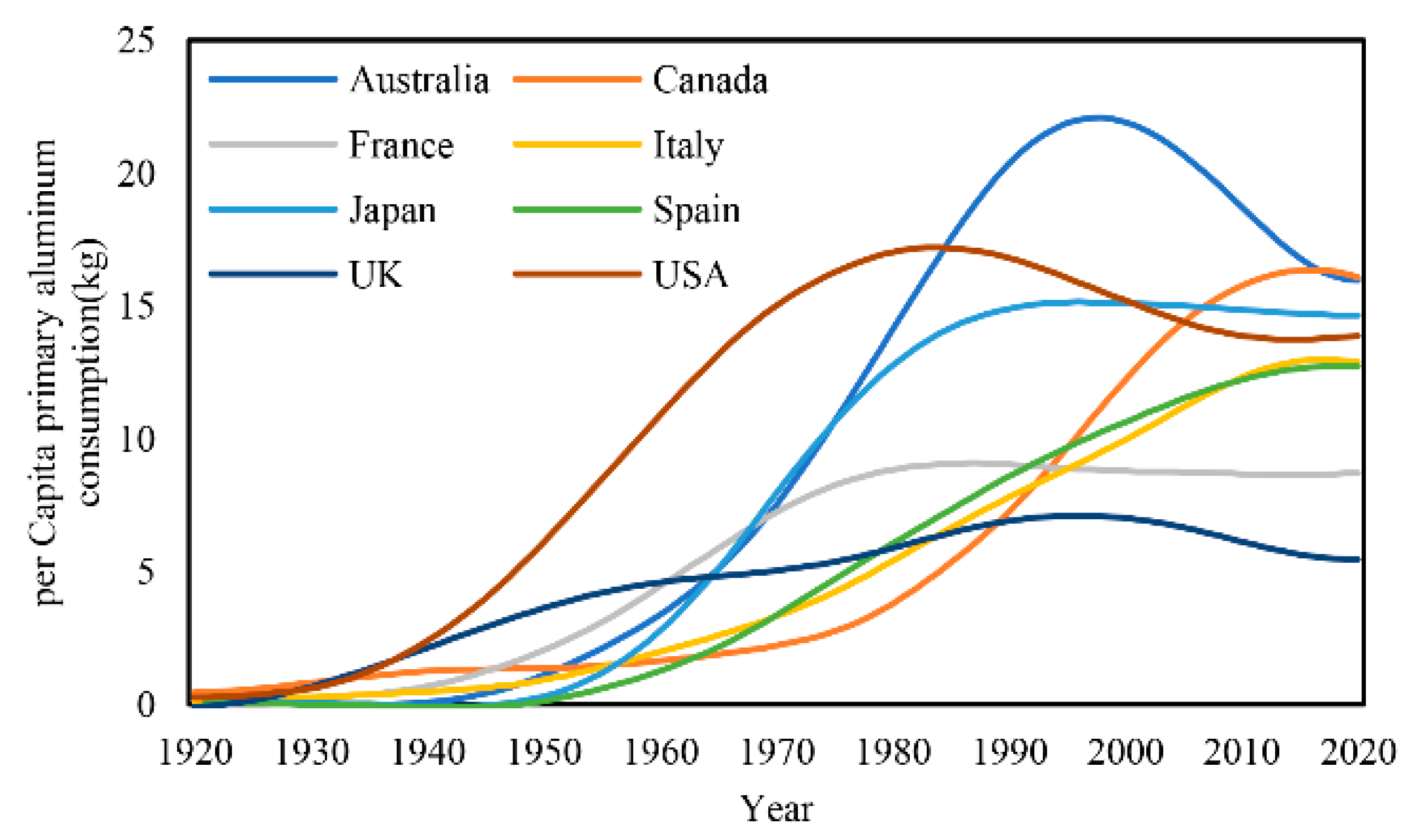
The results of the low-frequency components are shown in Figure 6 and Table S2. The low-frequency components show a fairly flat trend with little fluctuation and long period, contributing more than 70% to the volatility. The S-curve shows that the evolution of energy and mineral resources consumption is highly correlated with development of economy and society. Economic and social development, measured by GDP per capita, is the fundamental driving force for resource consumption. Applying the generalized equation of the S-curve, the primary aluminum consumptions of typical countries can be expressed (Figure S5, and Equation (S1)–(S8)).
The fitting results of low-frequency components and S-curves of typical countries show that their trajectories are highly consistent (Figure S6). Furthermore, the correlation between different economic development indicators and low-frequency components are analyzed, and the results are shown in Tables S3 and S4. The correlation coefficients of the S-curve and GDP per capita are the most significant.
Therefore, the influence of the low-frequency component on the volatility of primary aluminum consumption exceeds 70%, which dominates the long-term trend of primary aluminum consumption. This can be interpreted as economic development represented by GDP per capita, and the trend can be described by the S-curve.

3.4.2. Medium-Frequency Component

The results of the medium-frequency components are shown in Figure 7 and Table S5. The curves of medium-frequency components show the characteristics of large variations and long periods, contributing 2–16% of the volatility. Although the trajectory of resource and energy consumption in most developed economies at the macro level generally follows the S-curve model, the relationship between energy and mineral resource consumption and economy is affected by some significant events such as the oil crisis. These events may lead to different micro-evolution modes of per capita energy and mineral resource consumption in different economies.
In this study, the relationship between medium-frequency components and significant events is analyzed (Figure S7). There are some interesting features: (1) The shocks of significant events on the medium-frequency components can be generally observed, and the direction of effects are mostly consistent. For example, the oil crisis in 1973 and the financial crisis in 2008 caused the decline in primary aluminum consumption in most countries. (2) Due to the different policies and development levels of the aluminum industry, there may be great differences among the impacts of the same events. For example, in Japan, the Plaza Accord caused an obvious reduction of medium-frequency component from 2 kg to −3 kg, while other countries were rarely affected. Therefore, it is reasonable that the medium-frequency component can be interpreted by shocks from significant events.

3.4.3. High-Frequency Component

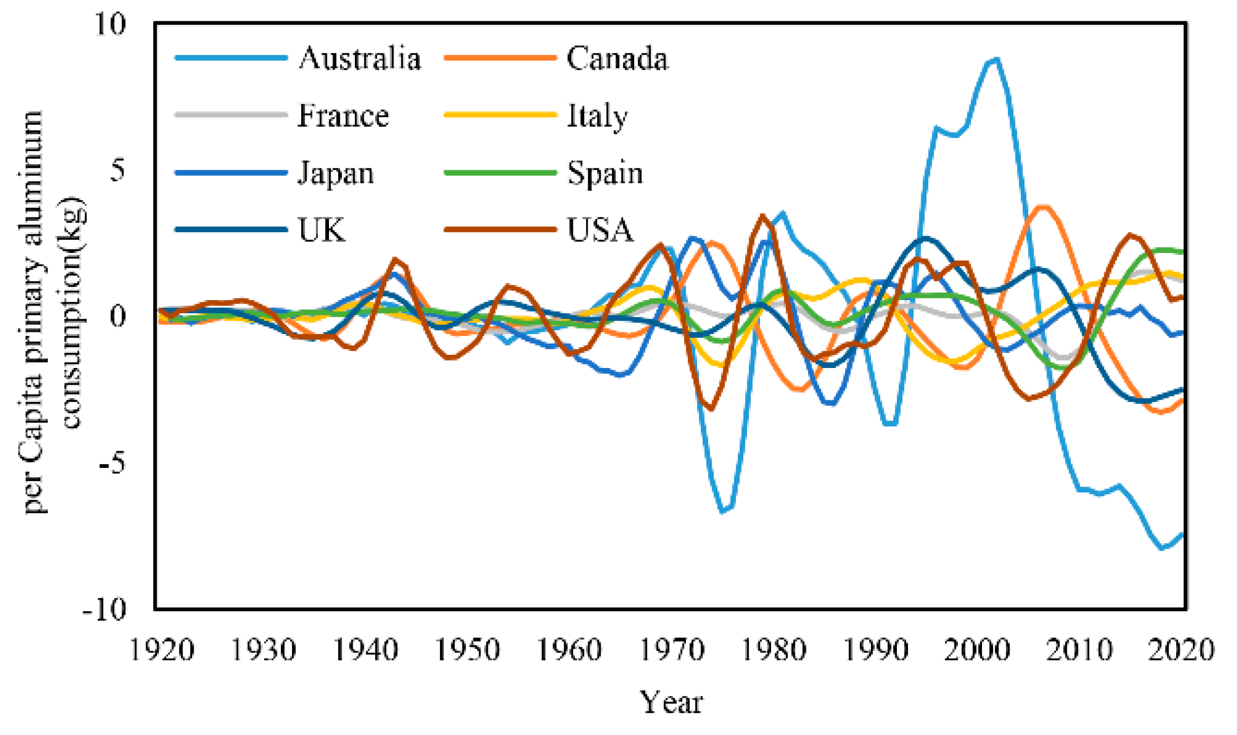
The results of the high-frequency components are shown in Figure 8 and Table S6. The curves of high-frequency components present complex series features, representing various short-term fluctuation factors. These high-frequency components have unsustainability, uncertain directions, and short periods, accounting for less than 9% of the total volatility.
Besides economic development and significant events, primary aluminum consumption is also influenced by many other factors, such as bad weather, strikes, and depletion of inventory. Durations of these effects are often short, and they can quickly return to the mean after a short period. So, they are classified into market disequilibrium events and their effects are contained in the high-frequency component. Although we call this component effects of normal market disequilibrium for short, it should be treated as a collection of events with short-term impact on primary aluminum consumption.
Normal market fluctuations, such as supply–demand imbalances, typically have a minor impact on primary aluminum consumption, generally no more than 2 kg. However, these events are becoming more frequent and are increasingly causing imbalances in supply and demand. As a result, normal market fluctuations can be neglected in long-term trend prediction, but they are important for short-term forecasting. Therefore, the high-frequency component is explained as normal supply–demand disequilibrium.

3.5. Model Test

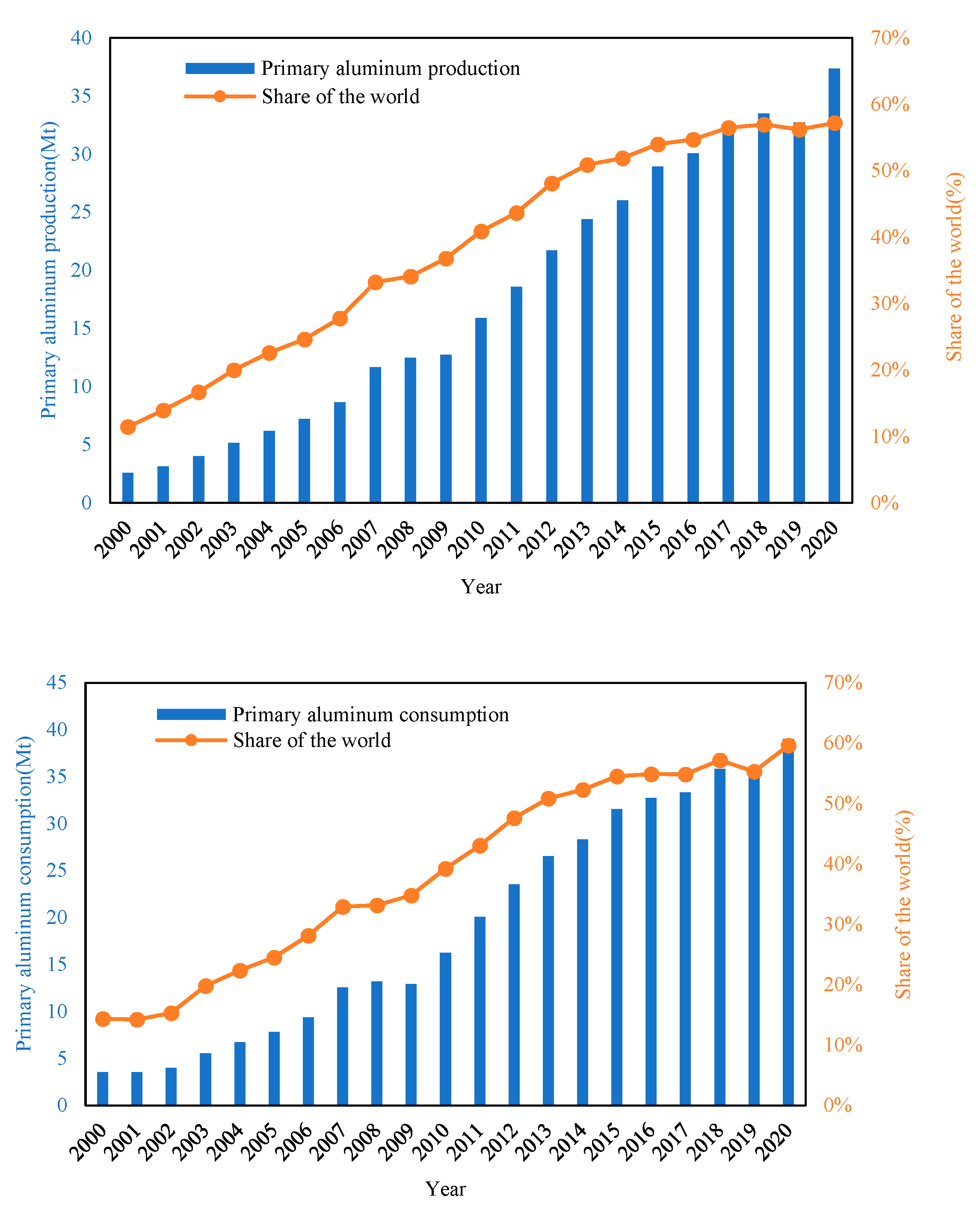
China, as a test country, is chosen for analysis in this study. Over the past two decades, China has dominated global aluminum production and consumption. Meanwhile, large amounts of CO2 have been released in China [47,48]. In 2020, China’s primary aluminum production and consumption exceeded 37 million tons and 39 million tons, respectively, accounting for more than half of the world’s production and consumption (Figure 9).
The decomposed results of the CEEMDAN-S-curve are shown in Figure 10, Figure S8, and Tables S7 and S8. The results of the analysis are presented as follows:
(1) Low-frequency component.
The low-frequency component exhibits a flat trend. The Pearson correlation, Kendall correlation, variance as % of observed, and variance as % of sum components of the original series are 0.94, 0.93, 60.77%, and 82.60%, respectively. This indicates that the long-term trend of primary aluminum consumption is also determined by the low-frequency component.
Moreover, the fitting result of the low-frequency component and S-curves shows a high degree of consistency in their trajectories (see Figure 11, Equation (S9), and Table 2). The correlation analysis between the low-frequency component and economic indicators reveals that the correlation coefficients between GDP per capita and the S-curve are both above 0.9, indicating a strong correlation between the low-frequency component and GDP per capita in China.
Therefore, in China, a low-frequency component can also be attributed to economic development, represented by GDP per capita.
(2) Medium-frequency component.
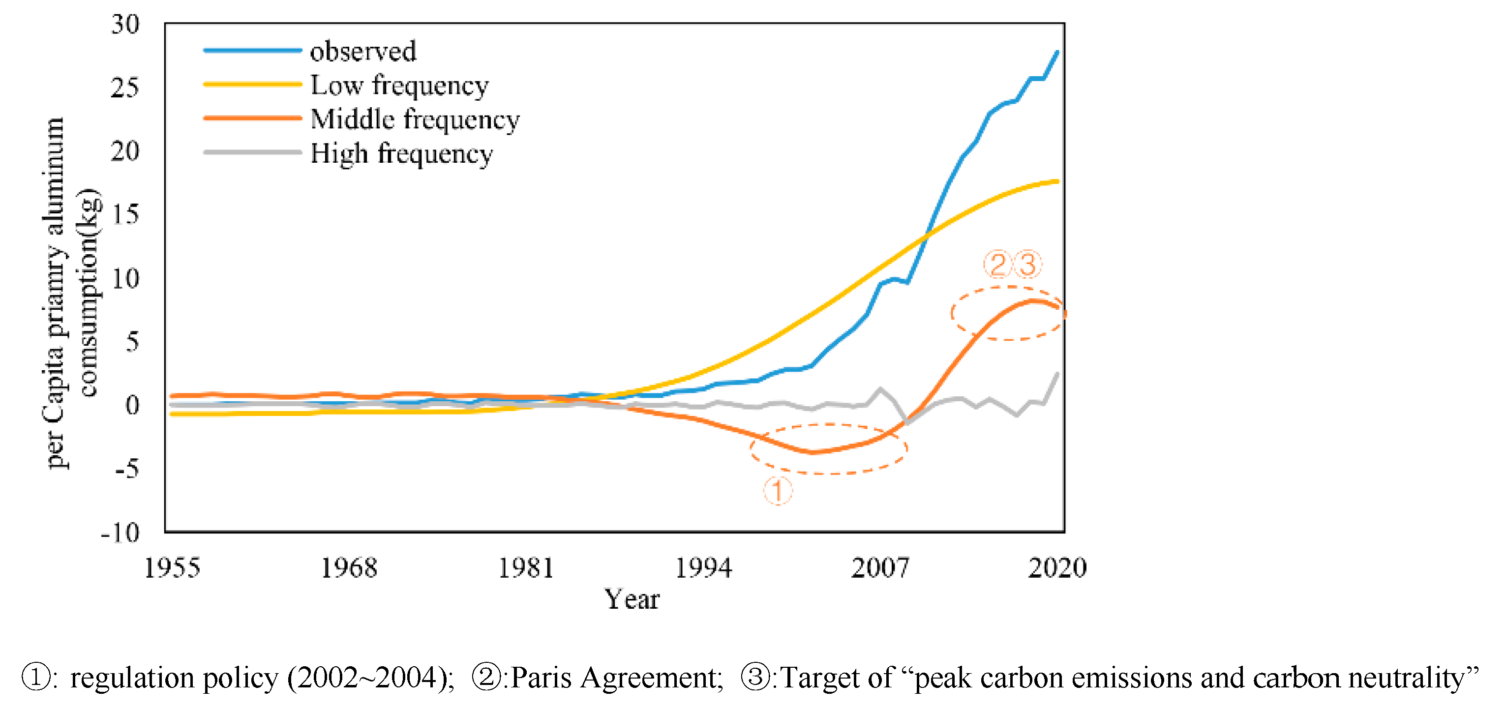
In China, the medium-frequency component has a large fluctuation and long period, contributing 2% to the volatility. Similarly, significant events, especially policies, have an obvious and long-lasting impact on the medium-frequency component. This result is consistent with the reality in China. For a long time, China has adhered to and can effectively implement the medium- and long-term plans to guide economic and social development. In 2002–2004, China introduced a series of aluminum regulation policies, which had a negative impact on the medium-frequency component. After that, the strong support for real estate and infrastructure construction became the main factor driving the rapid growth of consumption in the short term. With the signing of the Paris agreement, and achieving goals of carbon peak and carbon neutralization, primary aluminum consumption was limited. The occurrence time of these significant events coincides with the fluctuation trajectory of the medium-frequency component.
Therefore, in China, the medium-frequency component can be explained by the effect of significant events, represented by policies.
(3) High-frequency component.
In China, the high-frequency component comprises lower amplitudes and a short period, while the contribution is less than 1% to the volatility. Moreover, the amplitude of the high-frequency component in China is lower than in other typical countries, which is mainly related to government intervention. When there is a large fluctuation or volatility expectation in the market, the government-led mediation mechanism will implement various strategies to maintain the market balance. So, the high-frequency component can be explained by the normal market fluctuations of governmental intervention in China.
Therefore, the CEEMDAN-S-curve analysis results for China are consistent with those for typical countries, which proves that this model has good applicability and stability.

3.6. Final Results

Finally, the following results are obtained:
(1) It is reasonable that the time series of primary aluminum consumption can be decomposed into a low-frequency component, medium-frequency component, and high-frequency component. These contribute more than 70%, 2–17%, and less than 9% to consumption volatility, respectively.
(2) The long-term evolution of primary aluminum consumption is determined by the low-frequency component. Low-frequency component is viewed as economic development, represented by GDP per capita.
(3) The medium-frequency component leads to large fluctuations in primary aluminum consumption, which can be interpreted as the shocks of significant events.
(4) The short-term fluctuation of primary aluminum consumption is caused by high-frequency components. The high-frequency component can be interpreted as normal supply–demand disequilibrium.

3.7. Limitations

Despite the promising results, there are several limitations to the CEEMDAN-S-curve model that should be noted.
  • The analysis is highly dependent on abundant data, which can be challenging to obtain and process. This limitation may pose a challenge for researchers who do not have access to relevant data.
  • The application of the model needs to be adjusted to fit the specific status of different countries due to their varying levels of development. This may affect the accuracy of the results in some cases.
  • The CEEMDAN-S-curve model is designed to capture the impact of predictable factors on primary aluminum consumption and is not able to account for unexpected events or external shocks, which can have some impact on consumption patterns.

4. Discussion

4.1. Comparison between the CEEMDAN-S-Curve and Other Models

Based on previous literatures, this paper summarizes several major research models of aluminum consumption. As shown in Table 3, different models have merits and drawbacks. For instance, the life cycle analysis is easy to understand and can determine the stock and flow direction by studying the cycle of aluminum in the industrial chain [22]. However, this method can be time-consuming when accessing data [1,24]. Other methods may overlook the practical significance of data or overemphasize the experience of developed countries [18,28]. Additionally, the expert evaluation method, while simple and direct, may yield different conclusions from different experts [54].
Compared with the above models, CEEMDAN-S-curve model has the following obvious merits:
(1) The CEEMDAN-S-curve model decomposes primary aluminum consumption time series into different components and explains each component in a direct and quantitative way.
(2) The hybrid CEEMDAN-S-curve model combines the intelligent decomposition algorithm and the S-curve, which effectively overcomes the shortcomings of a single model and improves analytical capabilities.
(3) The results demonstrate that the CEEMDAN-S-curve model has good stability and applicability, as demonstrated in its analysis of nine typical countries over the last 100 years.
Furthermore, the possibility of applying the model to predict primary aluminum consumption is discussed. The forecast model of primary aluminum consumption can generally be divided into inflow-driven and stock-driven [55,56]. The inflow-driven model directly establishes the relationship between consumption and socio-economic indicators (i.e., urbanization rate and GDP), while the stock-driven model establishes the relationship between per capita consumption and socio-economic indicators, and then predicts consumption indirectly [12,18,57,58].
In this paper, the decomposition results of CEEMDAN-S-curve are low-frequency, medium-frequency, and high-frequency components. These three components established links with different indicators, such as the low-frequency component and GDP per capita (stock-driven), medium-frequency component and significant events (inflow-driven), high-frequency component and market imbalance (inflow-driven). Therefore, CEEMDAN-S-curve combines the inflow-driven and stock-driven approaches and can be used to predict primary aluminum consumption in different countries.
For example, in 2020, China’s per capita primary aluminum consumption was 27.75 kg, with the low-frequency, medium-frequency, and high-frequency components contributing 17.60 kg, 7.72 kg, and 2.43 kg, respectively. This level is roughly equivalent to the consumption level in Japan in 1980 [2,3,43,44,45]. At this stage, social development was still the primary driving force determining the primary aluminum consumption. Considering the difference between the economic cycles (medium-frequency component) and market fluctuations (high-frequency component) of both countries, it can be expected that the consumption of primary aluminum will continue to increase in the next ten years until the consumption level of industrialized countries reaches its peak.

4.2. Primary Aluminum Consumption, CO2 Emission, and Recovery

Aluminum consumption drives the development of the aluminum industry chain (Figure S9). With economic and social development, demand will continue to expand. In addition, the shift towards cleaner and more sustainable energy sources, such as lightweight vehicles and solar energy, will require even more aluminum. Therefore, it is necessary for different countries to obtain aluminum resources to meet their needs for social and economic development. Generally, the source of aluminum is the production of primary aluminum and the recycling of recycled aluminum. However, primary aluminum production is extremely energy- and emissions-intensive, which has attracted attention to mitigation strategies from the material side [24]. In contrast, compared to primary aluminum, secondary aluminum production can save 93% of energy, helping to reduce GHG emissions and eliminate other environmental impacts (Figure 12) [59,60].
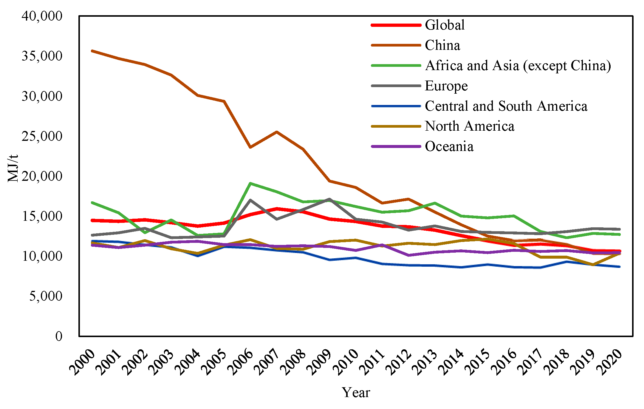
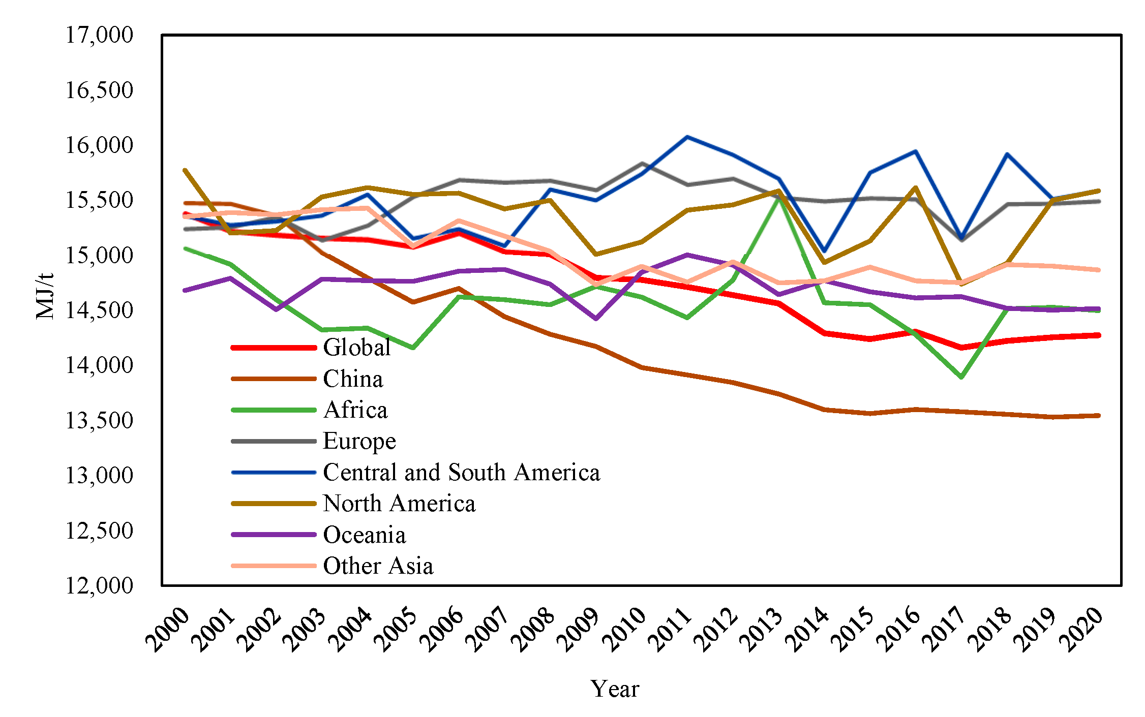
In 2020, the energy intensity of global aluminum production, including primary and secondary aluminum production, continued to decline. The production of primary aluminum involves two key steps: (1) alumina refining, which converts bauxite to alumina, and (2) aluminum smelting, which converts alumina to pure aluminum. The global energy intensity of alumina refining was 10,691 MJ/t in 2020, the lowest level in nearly 20 years. The energy intensity of global alumina refining increased from 14,479 MJ/t to 15,934 MJ/t from 2000 to 2007, and then began to decrease year by year. The energy intensity of global aluminum smelting was 14,273 kWh/t in 2020 (Figure 13). The energy intensity of global aluminum smelting decreased from 15,371 kWh/t to 14,161 kWh/t from 2000 to 2017, but it showed a slight upward trend in the following three years (Figure 14).
The decline in energy intensity of global aluminum production has mainly benefited from China’s development over the past 20 years. With the continuous growth of aluminum production capacity, China‘s aluminum production accounted for more than half of the world in 2020 [2]. At the same time, the strength of aluminum smelting has dropped significantly and is now at its best level. However, as China’s potential for further improving energy intensity is largely exhausted, the global average decline in energy intensity has slowed down since 2014.
To achieve a net zero emission scenario in 2050, the following two aspects are critical: (1) developing innovative alternative production methods that reduce the energy intensity of both primary and secondary aluminum production; (2) increasing the proportion of secondary aluminum utilization, reducing the loss of raw materials.
Innovative alternative production methods can play a key role in reducing the energy intensity of aluminum production. One promising approach is the use of renewable energy sources such as hydropower and solar energy in the production process. Additionally, the development of new technologies like inert anodes and advanced electrolysis can significantly decrease energy consumption and emissions in primary aluminum production. These methods can contribute to reducing the overall energy intensity of aluminum production while also supporting the global transition to cleaner energy.
Increasing the utilization of secondary aluminum is also an effective strategy. The proportion of secondary aluminum production has remained at 30–35% from 2000 to 2020, which is not enough to achieve a net zero emission path. To achieve a net zero emission path by 2050, the share of secondary aluminum production should reach 40% by 2050 [61]. Therefore, reusing waste and considering recycling when designing products are important.
According to the analysis results based on the CEEMDAN-S-curve model, economic development (represented by GDP per capita) is the fundamental driving force for determining the consumption of chromium ore. Currently, most developing countries are still far from reaching the peak of their consumption demand, which means that they will still need to consume large amounts of aluminum resources in the future. However, economic growth in these countries has not been decoupled from energy consumption, and blindly pursuing net zero emissions could lead to carbon lock-in, stranded assets, and economic losses [62].
To balance economic growth and carbon reduction strategies, practical recommendations are proposed in this study.
  • Governments and investors should increase their support for research and development of technology.
  • The aluminum industry should prioritize the development of production plans that reduce carbon emissions.
  • Participants in the aluminum industry chain, such as manufacturers, engineers, and construction companies, should use material efficiency strategies to reduce demand for aluminum.
  • Policymakers should adopt mandatory emission reduction policies to promote green transformation.
  • The collection and monitoring of relevant data are also crucial.

5. Conclusions

Aluminum is the globally most used nonferrous metal, and clarifying the primary aluminum consumption mechanism is important for economic development and reducing GHG emissions. In this paper, the consumption mechanism of primary aluminum was explored using the CEEMDAN-S-curve model. The results show that consumption series can be decomposed into low-frequency, medium-frequency, and high-frequency components, which contribute more than 70%, 2–17%, and less than 9% to the volatility of the original series, respectively. This can be explained as economic development, represented by GDP per capita, the shocks of significant events, and normal market activities, respectively. In the long run, primary aluminum consumption is determined by economic development. The sharp downs or ups of primary aluminum consumption are triggered by significant events. Otherwise, small fluctuations in the short term are mainly driven by normal market activities. In addition, CEEMDAN-S-curve model can also be used for demand forecasting. However, the model has limitations such as being data-intensive, requiring specific adjustments for different countries, and not accounting for unexpected factors.
The research results have implications for broader issues, and practical suggestions are proposed. On the one hand, the consumption of primary aluminum is closely linked to the goal of zero net industrial emissions. Therefore, measures should be taken to promote the efficient use of primary aluminum and reduce GHG emissions, such as increasing government and investor support for research and development technology, reducing the demand for primary aluminum by implementing material efficiency strategies, and prioritizing the development of production plans in the aluminum industry. On the other hand, since secondary resources can save 93% of energy compared to primary aluminum, efforts should be made to use and recycle scrap. This includes investing more funds in recycling technology development and improving public awareness of recycling by implementing laws and regulations.

Supplementary Materials

The following supporting information can be downloaded at: https://www.mdpi.com/article/10.3390/su15054228/s1, Additional data and information are included in the supplementary material.

Author Contributions

Conceptualization, Z.P.; methodology, Z.P.; software, Z.P.; validation, Z.P. and D.C.; formal analysis, Z.P. and Z.Z.; investigation, Z.P. and D.C.; resources, Z.P., Z.Z. and D.C.; data curation, Z.P.; writing—original draft preparation, Z.P.; writing—review and editing, Z.P. and Z.Z.; visualization, Z.P.; supervision, Z.P. and Z.Z.; project administration, Z.Z.; funding acquisition, Z.P. All authors have read and agreed to the published version of the manuscript.

Funding

This research was funded by Qinghai Salt Lake Industry Co., Ltd., and Institute of Mineral Resources, Chinese Academy of Geological Sciences, Grant No. HE 2221.

Institutional Review Board Statement

Not applicable.

Informed Consent Statement

Not applicable.

Data Availability Statement

Data are contained within the article.

Acknowledgments

The author sincerely gives thanks for the institutional support provided by the China Geological Survey.

Conflicts of Interest

The authors declare no conflict of interest.

References

  1. Liu, G.; Müller, D.B. Addressing sustainability in the aluminum industry: A critical review of life cycle assessments. J. Clean. Prod. 2012, 35, 108–117. [Google Scholar] [CrossRef]
  2. International Aluminum Institute (IAI). International Aluminum Statistics. Available online: https://international-aluminium.org/statistics/primary-aluminium-production/ (accessed on 10 June 2022).
  3. World Bureau of Metal Statistics (WBMS). Metals Database Service. Available online: https://world-bureau.co.uk/publications-services/metals-database/ (accessed on 10 June 2022).
  4. London Metal Exchange (LME). LME Aluminum. Available online: https://www.lme.com/en/Metals/Non-ferrous/LME-Aluminium#Historical+data (accessed on 10 July 2022).
  5. Yi, X.J.; Lu, Y.L.; He, G.Z.; Li, H.K.; Chen, C.C.; Cui, H.T. Global carbon transfer and emissions of aluminum production and consumption. J. Clean. Prod. 2022, 362, 132513. [Google Scholar] [CrossRef]
  6. Yta, B.; Ct, C. An assessment of using aluminum and magnesium on CO2 emission in European passenger cars. Clean. Prod. 2019, 247, 119120. [Google Scholar]
  7. Chen, W.Q.; Shi, L. Analysis of aluminum stocks and flows in mainland China from 1950 to 2009: Exploring the dynamics driving the rapid increase in China’s aluminum production. Resour. Conserv. Recycl. 2012, 68, 18–28. [Google Scholar] [CrossRef]
  8. Chen, W.Q.; Shi, L.; Qian, Y. Substance flow analysis of aluminum in mainland China for 2001, 2004 and 2007: Exploring its initial sources, eventual sinks and the pathways linking them. Resour. Conserv. Recycl. 2010, 54, 557–570. [Google Scholar] [CrossRef]
  9. Monica, D.; Saptarshi, M. An outlook into energy consumption in large scale industries in India: The cases of steel, aluminum and cement. Energy Policy 2010, 11, 7286–7298. [Google Scholar]
  10. Li, S.; Zhang, T.; Niu, L.; Yue, Q. Analysis of the development scenarios and greenhouse gas (ghg) emissions in china’s aluminum industry till 2030. J. Clean. Prod. 2021, 290, 125859. [Google Scholar] [CrossRef]
  11. Du, J.D.; Han, W.J.; Peng, Y.H.; Gu, C.C. Potential for reducing GHG emissions and energy consumption from implementing the aluminum intensive vehicle fleet in china. Energy 2010, 35, 4671–4678. [Google Scholar] [CrossRef]
  12. Zhang, Y.; Sun, M.; Hong, J.; Han, X.; He, J.; Shi, W.; Li, X. Environmental footprint of aluminum production in China. J. Clean. Prod. 2016, 133, 1242–1251. [Google Scholar] [CrossRef]
  13. Linda, W. Trends and developments in long-term steel demand–the intensity-of-use hypothesis revisited. Resour. Policy 2014, 39, 134–143. [Google Scholar]
  14. Müller, D.B. Stock dynamics for forecasting material flows-case study for housing in The Netherlands. Ecol. Econ. 2006, 59, 142–156. [Google Scholar] [CrossRef]
  15. Menzie, W.D.; Barry, J.J.; Bleiwas, D.I.; Bray, E.L.; Goonan, T.G.; Matos, G. The Global Flow of Aluminum from 2006 through 2025. 2010. Available online: https://pubs.usgs.gov/of/2010/1256/ (accessed on 20 June 2022).
  16. Schipper, B.W.; Lin, H.C.; Meloni, M.A.; Wansleeben, K.; Heijungs, R.; van der Voet, E. Estimating global copper demand until 2100 with regression and stock dynamics. Resour. Conserv. Recycl. 2018, 132, 28–36. [Google Scholar] [CrossRef]
  17. Jia, H.X.; Li, T.J.; Wang, A.J.; Liu, G.W.; Guo, X.Q. Decoupling analysis of economic growth and mineral resources consumption in China from 1992 to 2017: A comparison between tonnage and exergy perspective. Resour. Policy 2021, 74, 102448. [Google Scholar] [CrossRef]
  18. Zhang, Z.Z.; Jiang, G.Y.; Wang, X.W.; Zhang, J.F. Development and Utilization of the World’s and China’s Bulk Mineral Resources and their Supply and Demand Situation in the Next Twenty Years. Acta Geol. Sin. Engl. Ed. 2016, 90, 1370–1417. [Google Scholar]
  19. Jiang, G.Y. Proceedings of the 2018 7th International Conference on Energy and Environmental Protection. Adv. Eng. Res. 2018, 9, 1363–1367. [Google Scholar]
  20. Liu, G.; Bangs, C.E.; Müller, D.B. Stock dynamics and emission pathways of the global aluminum cycle. Nat. Clim. Chang. 2013, 3, 338–342. [Google Scholar] [CrossRef]
  21. Pauliuk, S.; Wang, T.; Müller, D.B. Moving toward the circular economy: The role of stocks in the Chinese steel cycle. Environ. Sci. Technol. 2012, 46, 148–154. [Google Scholar] [CrossRef] [Green Version]
  22. Müller, E.; Hilty, L.M.; Widmer, R.; Schluep, M.; Faulstich, M. Modeling metal stocks and flows: A review of dynamic material flow analysis methods. Environ. Sci. Technol. 2014, 48, 2102–2113. [Google Scholar] [CrossRef] [PubMed]
  23. Dai, M.; Wang, P.; Chen, W.Q.; Liu, G. Scenario analysis of China’s aluminum cycle reveals the coming scrap age and the end of primary aluminum boom. J. Clean. Prod. 2019, 226, 793–804. [Google Scholar] [CrossRef]
  24. Li, Q.F.; Dai, T.; Gao, T.M.; Zhong, W.Q.; Wen, B.J.; Li, T.B.; Zhou, Y.J. Aluminum material flow analysis for production, consumption, and trade in China from 2008 to 2017. J. Clean. Prod. 2021, 296, 126444. [Google Scholar] [CrossRef]
  25. Niaz, B.B.; Ramos, P.M. Crude Oil Price Forecasting Techniques: A Comprehensive Review of Literature. SSRN Electron. J. 2013, 7, 1–32. [Google Scholar] [CrossRef]
  26. Neha, S.; Krishan, K.P. Artificial intelligence methods for oil price forecasting: A review and evaluation. Energy Syst. 2015, 6, 479–506. [Google Scholar]
  27. Fernando, S.L.; Francisco, C.J.; Ana, S.S.; Alicja, K.; Pedro, R.F. Forecasting the COMEX copper spot price by means of neural networks and ARIMA models. Resour. Policy 2015, 45, 37–43. [Google Scholar]
  28. Yan, X.J.; Luo, J.C.; Chen, Z.Y. Forecasting of the Demand of Alumina Based on the Coupling Phase-space Reconstruction and Neural Network. Int. J. Bus. Manag. 2010, 5, 146–153. [Google Scholar] [CrossRef] [Green Version]
  29. Xu, G.D.; Ao, H.; She, Y.G. Research on the consumption law of primary aluminum and prediction of consumption in China. China Man Inf. 2013, 16, 31–35. (In Chinese) [Google Scholar]
  30. Yuan, W.F.; Zheng, M.G. Scenario analysis of China’s aluminum resource demand based on BP neural network. Res. Ind. 2014, 16, 132–137. (In Chinese) [Google Scholar]
  31. Ahmed, A.E.; Mohamed, A.E.; Zakaria, A.; Ye, H.W.; Zhang, J.H. Improving multilayer perceptron neural network using chaotic grasshopper optimization algorithm to forecast iron ore price volatility. Resour. Policy 2020, 65, 101555. [Google Scholar]
  32. Wu, Z.H.; Huang, N.E. Ensemble empirical mode decomposition: A noise-assisted data analysis method. Adv. Adapt. Data Anal. 2009, 1, 1–41. [Google Scholar] [CrossRef]
  33. Li, H.Z.; Guo, S.; Li, C.J.; Sun, J.Q. A hybrid annual power load forecasting model based on generalized regression neural network with fruit fly optimization algorithm. Knowledge-Based Syst. 2013, 37, 378–387. [Google Scholar] [CrossRef]
  34. Wang, A.J.; Wang, G.S.; Chen, Q.S.; Yu, W.J.; Yan, K.; Yang, H.B. S-curve model of relationship between energy consumption and economic development. Nat. Resour. Res. 2015, 24, 53–64. [Google Scholar] [CrossRef]
  35. Tsoularis, A.; Wallace, J. Analysis of logistic growth models. Math. Biosci. 2002, 179, 21–55. [Google Scholar] [CrossRef] [Green Version]
  36. Colominas, M.A.; Schlotthauer, G.; Torres, M.E. Improved complete ensemble EMD: A suitable tool for biomedical signal processing. Biomed. Signal Process. Control 2014, 14, 19–29. [Google Scholar] [CrossRef]
  37. Wang, Y.M.; Gu, J.Z.; Zhou, Z.L.; Wang, Z.J. Diarrhoea outpatient visits prediction based on time series decomposition and multi-local predictor fusion. Knowledge-Based Syst. 2015, 88, 12–23. [Google Scholar] [CrossRef]
  38. Torres, M.E.; Colominas, M.A.; Schlotthauer, G.; Flandrin, P. A complete ensemble empirical mode decomposition with adaptive noise. In Proceedings of the IEEE International Conference on Acoustics, Speech and Signal Processing (ICASSP), Toronto, ON, Canada, 6–11 June 2021. [Google Scholar]
  39. Gao, X.R.; Wang, A.J.; Liu, G.W.; Liu, C.H.; Yan, K. Expanded S-Curve Model of a Relationship Between Crude Steel Consumption and Economic Development: Empiricism from Case Studies of Developed Economies. Nat. Resour. Res. 2018, 28, 547–562. [Google Scholar] [CrossRef]
  40. Lempel, A.; Ziv, J. On the complexity of finite sequences. IEEE Trans. Inf. Theory. 1976, 22, 75–81. [Google Scholar] [CrossRef]
  41. British Geological Survey (BGS). UK and World Mineral Statistics Datasets. Available online: https://www.bgs.ac.uk/geological-data/ (accessed on 20 June 2022).
  42. U.S. Geological Survey (USGS). Aluminum Statistics and Information. Available online: https://minerals.usgs.gov/minerals/pubs/commodity/aluminum/ (accessed on 10 June 2022).
  43. The World Bank (WB). World Bank Open Data. Available online: https://data.worldbank.org/ (accessed on 10 June 2022).
  44. United Nations (UN). World Population Prospects. Available online: https://population.un.org/wpp/DataQuery/ (accessed on 10 June 2022).
  45. Groningen Growth and Development Centre (GGDC). Total Economy Database. Available online: http://www.ggdc.net (accessed on 10 June 2022).
  46. Zhang, X.; Lai, K.K.; Wang, S.Y. A new approach for crude oil price analysis based on Empirical Mode Decomposition. Energy Econ. 2008, 30, 905–918. [Google Scholar] [CrossRef]
  47. Lin, B.Q.; Wang, M. The role of socio-economic factors in China’s CO2 emissions from production activities. Sustain. Prod. Consum. 2021, 27, 217–227. [Google Scholar] [CrossRef]
  48. Xia, Q.; Tian, G.L.; Wu, Z. Examining embodied carbon emission flow relationships among different industrial sectors in China. Sustain. Prod. Consum. 2022, 29, 100–114. [Google Scholar] [CrossRef]
  49. China Nonferrous Metal Industry Association. Industry Data. Available online: https://www.chinania.org.cn/html/hangyetongji/chanyeshuju/ (accessed on 10 June 2022).
  50. National Bureau of Statistics of China. National Data. Available online: https://data.stats.gov.cn/ (accessed on 10 June 2022).
  51. Ministry of Industry and Information Technology of China. Statistical Analysis. Available online: https://www.miit.gov.cn/gxsj/tjfx/yclgy/ys/index.html (accessed on 10 June 2022).
  52. Ministry of Natural Resources of China. Data Service. Available online: http://www.mnr.gov.cn/sj/sjfw/ (accessed on 10 June 2022).
  53. General Administration of Customs of China. Customs Statistics. Available online: http://www.customs.gov.cn/ (accessed on 10 June 2022).
  54. Li, X.; Zhang, X. Analysis of aluminum supply and demand development trend in China and the United States. Adv. Mater. Res. 2014, 962–965, 1936–1942. [Google Scholar] [CrossRef]
  55. Graedel, T.E.; Barr, R.; Chandler, C.; Chase, T.; Choi, J.; Christoffersen, L.; Friedlander, E.; Henly, C.; Jun, C.; Nassar, N.T.; et al. Methodology of metal criticality determination. Environ. Sci. Technol. 2012, 46, 1063–1070. [Google Scholar] [CrossRef]
  56. Bleischwitz, R.; Nechifor, V.; Winning, M.; Huang, B.; Geng, Y. Extrapolation or saturation—Revisiting growth patterns, development stages and decoupling. Glob. Environ. Chang. 2018, 48, 86–96. [Google Scholar] [CrossRef]
  57. Watari, T.; Nansai, K.; Nakajima, K. Review of critical metal dynamics to 2050 for 48 elements. Resour. Conserv. Recycl. 2020, 155, 104669. [Google Scholar] [CrossRef]
  58. Watari, T.; Nansai, K.; Nakajima, K. Major metals demand, supply, and environmental impacts to 2100: A critical review. Resour. Conserv. Recycl. 2021, 164, 105107. [Google Scholar] [CrossRef]
  59. Jerry, B.; Patrik, S. The economics of secondary aluminum supply: An econometric analysis based on European data. Resour. Conserv. Recycl. 2009, 53, 455–463. [Google Scholar]
  60. Zink, T.; Geyer, R.; Startz, R. Toward estimating displaced primary production from recycling: A case study of U.S. Aluminum. J. Ind. Ecol. 2018, 22, 314–326. [Google Scholar] [CrossRef]
  61. IEA. Aluminum. Available online: https://www.iea.org/reports/aluminium (accessed on 10 June 2022).
  62. De, L.L.; Guo, R.; Cao, X.J.; Ni, X.J.; Zhang, W. Accelerating the energy transition to achieve carbon neutrality. Resour. Conserv. Recycl. 2022, 177, 105977. [Google Scholar]
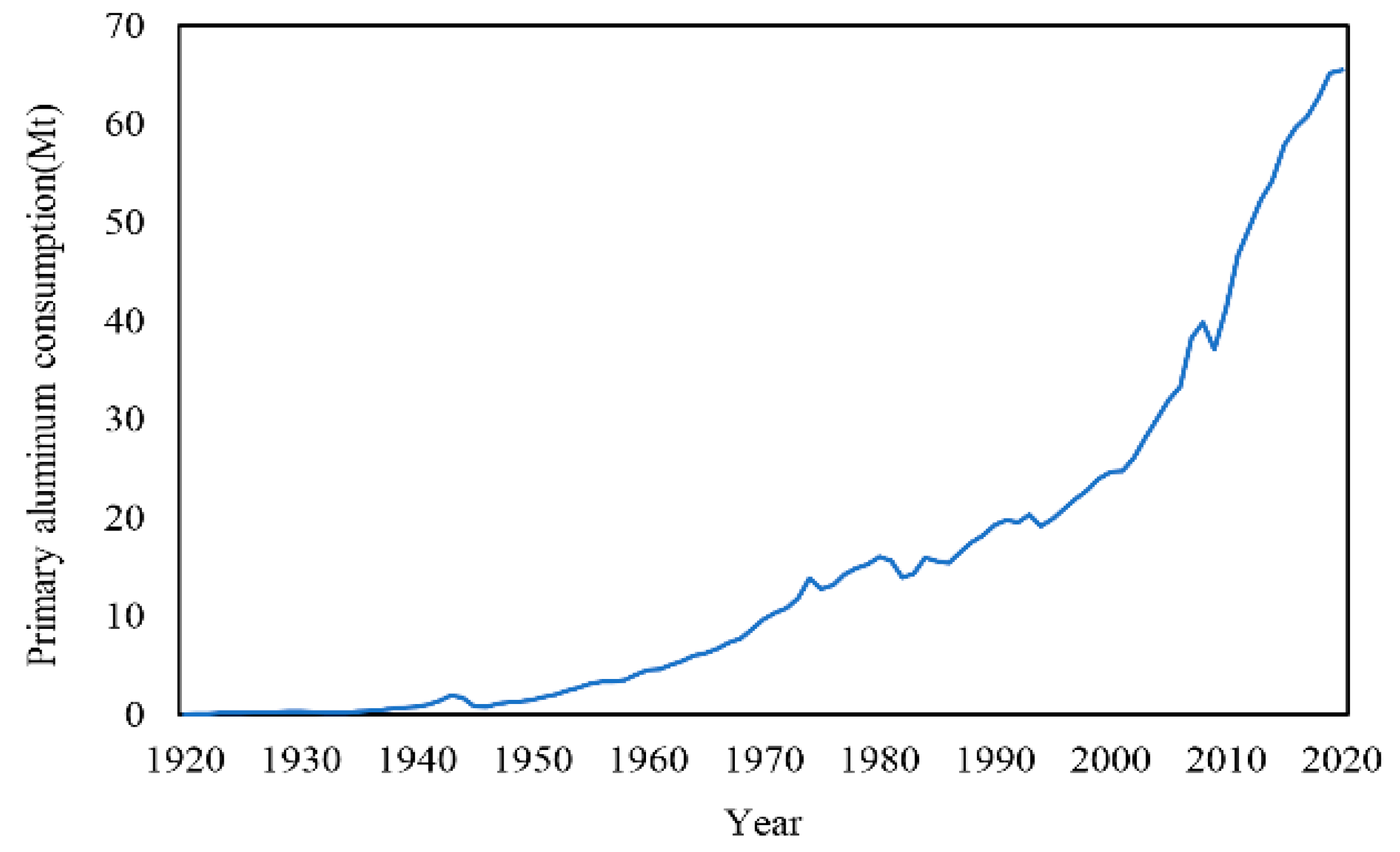
Figure 1. Global primary aluminum consumption from 1920 to 2020. Source: IAI [2].
Sustainability 15 04228 g001
Figure 2. Growth rate and three changing points of per capita energy and mineral resources consumption.
Sustainability 15 04228 g002
Figure 3. The proposed CEEMDAN-S-curve model framework.
Sustainability 15 04228 g003
Figure 4. Primary aluminum consumption in typical countries from 1920 to 2020. Source: IAI [2], WBMS [3], BGS [41], USGS [42].
Sustainability 15 04228 g004
Figure 5. Per capita primary aluminum consumption of typical countries. Source: IAI [2], WBMS [3], WB [43], UN [44], GGDC [45].
Sustainability 15 04228 g005
Figure 6. Low-frequency components for per capita primary aluminum consumption of typical countries.
Sustainability 15 04228 g006
Figure 7. The medium-frequency components for per capita primary aluminum consumption of typical countries.
Sustainability 15 04228 g007
Figure 8. The high-frequency components for per capita primary aluminum consumption of typical countries.
Sustainability 15 04228 g008
Figure 9. The production, consumption, and world share of primary aluminum in China from 2000 to 2020. Source: China Nonferrous Metal Industry Association [49], National Bureau of Statistics of P.R. China [50], Ministry of Industry and Information Technology of P.R. China [51].
Sustainability 15 04228 g009
Figure 10. The components for the primary aluminum consumption in China. Source: China Nonferrous Metal Industry Association [49], National Bureau of Statistics of P.R. China [50], Ministry of Industry and Information Technology of P.R. China [51], Ministry of Natural Resources of P.R. China [52], General Administration of Customs of P.R. China [53].
Sustainability 15 04228 g010
Figure 11. Observed, S-curve simulation, and low-frequency component of per capita primary aluminum consumption in China. Relationship between observed and S-curve simulation (a), and connection between observed, S-curve simulation, and low-frequency component from 1955 to 2020 (b).
Sustainability 15 04228 g011
Figure 12. Greenhouse gas emissions from different aluminum sectors in 2019. Source: IAI [2].
Sustainability 15 04228 g012
Figure 13. Energy intensity of alumina refining by region from 2000–2020. Source: IAI [2].
Sustainability 15 04228 g013
Figure 14. Energy intensity of primary aluminum smelting by region from 2000–2020. Source: IAI [2].
Sustainability 15 04228 g014
Table 1. Reconstruction results of IMFs and the residue.
CountryHigh-FrequencyMedium-FrequencyLow-Frequency
AustraliaIMF1, IMF2IMF3, IFM4, IMF5Res
CanadaIMF1, IMF2, IMF3IMF4, IMF5Res
FranceIMF1, IMF2, IMF3IMF4, IMF5IMF6, Res
ItalyIMF1, IMF2, IMF3IMF4, IMF5Res
JapanIMF1, IMF2IMF3, IFM4, IMF5Res
SpainIMF1, IMF2, IMF3IMF4, IMF5Res
UKIMF1, IMF2, IMF3IMF4, IMF5Res
USAIMF1, IMF2IMF3, IMF4, IMF5IMF6, Res
Table 2. Pearson correlation and Kendall correlations between low-frequency component and different economic indicators in China.
GPCS-CurveURIVAPCEPCOME
Pearson correlation0.98 *0.93 *0.99 *0.160.98 *−0.69 *
Kendall correlation0.96 *0.96 *0.92 *0.23 *1.00 *−0.49 *
Note: GPC = GDP per capita, UR = Urbanization rate, IVA = Industry value added (% of GDP), PCEPC = per capita electric power consumption, OME = Ore and metal export (% of merchandise exports); *: Correlation is significant at 0.05 level.
Table 3. Major models for analyzing aluminum consumption.
CategorySpecific MethodsMerits and DrawbacksCore Data
Hybrid modelCEEMDAN-S-curveMerits: quantitative analysis;
evaluated directly; combining the merits of different models; clear, stable, and reliable results
Drawbacks: difficult to access data
major economic and social
indicators, significant events, market price, policy
Market survey methodSector analysis method [55]Merits: clear; solid theoretical foundation; easy to master; reliable results
Drawbacks: difficult to access data; complex downstream subdivision
consumption data of different downstream sectors
Life cycleMaterial flow analysis [1,22,24]Merits: solid theoretical foundation; easy to master; evaluated directly
Drawbacks: difficult to access data; complex downstream subdivision
parameters of virous flows
Mathematical modelNeural Network [28]Merits: simple and easy to operate; reliable results
Drawbacks: easy to ignore realistic social factors
per capita consumption
S-curve [18,19]Merits: scenario analysis, quantitative analysis; easy to explain indicators
Drawbacks: too dependent on the developed country pattern
per capita consumption,
per capita GDP,
population,
economic growth rate
Expert experience methodExpert forecasting method [49]Merits: rich experience, strong analytical capability
Drawbacks: not objective enough
experts’ judgment
Disclaimer/Publisher’s Note: The statements, opinions and data contained in all publications are solely those of the individual author(s) and contributor(s) and not of MDPI and/or the editor(s). MDPI and/or the editor(s) disclaim responsibility for any injury to people or property resulting from any ideas, methods, instructions or products referred to in the content.