Article

Artificial Intelligence for the Detection of Asbestos Cement Roofing: An Investigation of Multi-Spectral Satellite Imagery and High-Resolution Aerial Imagery

by
Mia V. Hikuwai
1,2,*,
Nicholas Patorniti
2,3,
Abel S. Vieira
1,2,
Georgia Frangioudakis Khatib
4 and
Rodney A. Stewart
1,3
1
Griffith School of Engineering and Built Environment, Griffith University, Parklands Drive, Southport, QLD 4222, Australia
2
UACS Consulting Pty Ltd., 12/102 Burnett Street, Buderim, QLD 4556, Australia
3
Cities Research Institute, Griffith University, Parklands Drive, Southport, QLD 4222, Australia
4
Australian Government Asbestos Safety and Eradication Agency, Surry Hills, NSW 2010, Australia
*
Author to whom correspondence should be addressed.
Sustainability 2023, 15(5), 4276; https://doi.org/10.3390/su15054276
Submission received: 27 November 2022 / Revised: 21 February 2023 / Accepted: 24 February 2023 / Published: 27 February 2023

Abstract

:
Artificial Intelligence (AI) is providing the technology for large-scale, cost-effective and current asbestos-containing material (ACM) roofing detection. AI models can provide additional data to monitor, manage and plan for ACM in situ and its safe removal and disposal, compared with traditional approaches alone. Advances are being made in AI algorithms and imagery applied to ACM detection. This study applies mask region-based convolution neural networks (Mask R-CNN) to multi-spectral satellite imagery (MSSI) and high-resolution aerial imagery (HRAI) to detect the presence of ACM roofing on residential buildings across an Australian case study area. The results provide insights into the challenges and benefits of using AI and different imageries for ACM detection, providing future directions for its practical application. The study found model 1, using HRAI and 460 training samples, was the more reliable model of the three with a precision of 94%. These findings confirm the efficacy of combining advanced AI techniques and remote sensing imagery, specifically Mask R-CNN with HRAI, for ACM roofing detection. Such combinations can provide efficient methods for the large-scale detection of ACM roofing, improving the coverage and currency of data for the implementation of coordinated management policies for ACM in the built environment.

1. Introduction

The global industrialisation of asbestos occurred rapidly over a 150-year period as its conductivity, fire-proofing and strengthening properties became valuable in the construction and manufacturing industries. Now, asbestos-related diseases cause an estimated 255,000 global deaths annually [1,2]. Responding to the prevalence of asbestos-related diseases, the use and distribution of asbestos and asbestos-containing materials (ACMs) is banned in over 60 countries as of 2020 [2].
Asbestos is a hazardous substance [3]. When asbestos is disturbed, or ACMs become damaged, disturbed or are deteriorating, microscopic silicate fibres can become airborne. Inhalation exposure to these airborne fibres can cause asbestos-related diseases such as asbestosis, lung cancer, and mesothelioma [3,4]. Disturbance activities which can lead to asbestos exposure include but are not limited to unsafe ACM management practices during home improvement and redevelopment, disaster events, illegal dumping and weathering [5].
This paper focuses on the Australian asbestos problem as an archetype case study for the broader application of artificial intelligence (AI) for ACM detection both domestically and in other countries. Asbestos was completely banned in Australia from the end of 2003, but a large legacy of ACMs remains in the built environment. New approaches to more effectively manage the legacy ACM remaining in situ, and plan for its safe removal and disposal are needed. To aid in developing these new approaches, the Australian Government Asbestos Safety and Eradication Agency (ASEA) was established in 2013 to coordinate the implementation of the National Strategic Plan for Asbestos Management and Awareness (Asbestos National Strategic Plan). The current phase of the Asbestos National Strategic Plan contains a target of developing an evidence-based national picture that assesses the likelihood of ACMs being present in the residential environment. ACM identification is a key national priority of this plan, as locating ACM provides the means to estimate quantities and plan for safe management in situ, before removal and disposal. This study was undertaken in conjunction with ASEA. Australia is a suitable case study for AI detection of ACMs, as asbestos-related diseases are responsible for over 4000 Australian deaths every year [6], and there are an estimated 6.2 million tonnes of ACM remaining in the Australian built environment [7].
To ultimately reduce the cases of exposure, individuals and policymakers require information about the location and quantity of ACMs [8,9]. Traditional methods to detect asbestos are costly and time-consuming, requiring physical sampling in situ, laboratory testing and extended waiting periods for results [10]. Current data about the location of ACMs in the residential environment is scattered and incomplete, and traditional methods are difficult to implement on a large scale while maintaining currency. Large-scale detection methods for ACM roofing are being investigated across the world and generally utilise remote sensing imageries such as multi-spectral resolution imagery (MSSI) and high-resolution aerial imagery (HRAI), combined with AI technologies [8]. As most ACMs are reaching the end of their product life and can begin deteriorating, there is an elevated risk for asbestos exposure from the release of airborne asbestos fibres. ACM roofing can be difficult to maintain, as it is not as easily monitored and accessible as ground-level ACMs are. Remote sensing imagery allows for ACM roofing to be easily detected at a large scale, contributing to efforts to prevent exposure to asbestos fibres.
This research will utilise remote sensing imageries and advanced AI to explore its efficacy to detect ACM roofing and the variability of the AI models in this space. The aim of this study is to investigate the use of MSSI and HRAI with an AI called mask region-based convolutional neural network (Mask R-CNN) for the detection of ACM roofing in the residential building stock of a case study area in Australia.

1.1. Asbestos in Australia

The manufacture, use, reuse, import, transport, storage or sale of all forms of asbestos was banned in Australia from 2003 [7]. Prior to that, Australia was one of the highest consumers of asbestos per capita during its peak production in the 1900s. It now deals with a legacy issue of ACM in situ throughout government, commercial and residential building stock. It is estimated that 1.9 million tonnes of asbestos were consumed in Australia between 1920–2003 [7].
A residential-focused case study area was chosen for this Australian study as while more is known about the level of ACMs present in public and commercial buildings, less is known about the residential building stock. Nation-wide, ‘workplaces’ built before certain dates are required to use an asbestos register that lists areas of confirmed or assumed asbestos in the building, whereas this is not a requirement for almost all residential buildings [11].
In residential buildings, roofing, eaves, walls, tiles and fences are just some products that could contain asbestos. Before the 1960s, 25% of residential buildings in Australia used ACM sheeting externally, internally and for roofing [7]. Recent studies estimate that 1 in 3 houses contain some type of ACM; however, there is limited data on the density and location of affected houses in Australia [12]. Successful large-scale ACM detection and asbestos identification for Australian residential buildings would have a great impact on the overall health of Australian communities as there is a lack of existing data for residential buildings and high volumes of ACM that remain in situ.

1.2. Asbestos Identification vs. ACM Detection

In Australia, workplace health and safety laws provide that only an asbestos test performed in an accredited laboratory can be used to identify asbestos in a material [11]. Furthermore, only the National Association of Testing Authorities (NATA) accredits laboratories for asbestos testing. The traditional asbestos testing method requires physical sampling and at least polarised light microscopy, in accordance with Australian Standard AS4964-2004 [13]. This is a time-consuming and expensive method due to the workforce and equipment required [9,10] and is inefficient when considering ACM detection on a large scale. Advancements in technology and accessibility, and investigations into other methods of ACM detection are being carried out across the world. These represent complementary approaches to asbestos identification that can be used to inform on-the-ground asbestos assessment and testing, validate the outputs from new technology or inform where to prioritise asbestos management action.
The use of AI and imagery for large-scale ACM detection has increased as remote sensing imagery has become more cost efficient, greater coverage and better temporal currency. Published studies using AI and imagery for ACM roof detection have included methods combining remote sensing imagery with object detection and pixel classification-based AI algorithms [8]. Advancements in machine learning (specifically deep learning) have provided opportunities to improve object detection, therefore improving the ability to detect ACM roofing [14,15]. These methods are more sophisticated and efficient for large-scale asbestos detection compared to the traditional methods and are now starting to be used in practice; however, there are still areas for improvement. Studies that used MSSI and hyperspectral satellite imagery (HSSI) were restricted due to the lower spatial resolutions available for that type of imagery [16]. Generally, previous studies used classification algorithms that were primarily pixel based. However, a 2008 study by Weih and Riggan [17] highlighted the increase in accuracy of object detection methods when using HRAI, as opposed to MSSI. One study identified in the literature explored the use of remote sensing imagery and convolutional neural networks (CNN) to detect ACM roofing focusing on the use of aerial hyper-spectral and multi-spectral imagery [10]. Similar studies [9,10,14,15,16,18,19] present evidence for the efficacy of using remote sensing and AI methods to detect ACM roofing; however, there is an opportunity to advance and expand upon the existing works regarding the best practice of large-scale asbestos detection and management. Expanding these works can be accomplished by investigating existing studies for limitations, making new adjustments to methods or using newer data inputs, since changes in these areas can enhance modelling outputs. For example, in 2016, Toth and Jóźków [20] remarked on the advancements occurring in remote sensing technology, which has resulted in improved resolution availability, spectral capacity, coverage and accessibility [21]. The advancements in remote sensing capabilities, and the data and information that can now be captured provides the opportunity for more in-depth research to be accomplished [18,19,20]. Toth and Jóźków [20] also commented on the necessity for improving methods to be able to process and analyse these enhanced datasets and information. In other research areas, studies have focused on advancing CNN frameworks and capabilities, allowing for more adaptable hyperparameters (e.g., number of training cycles) to improve model performance of processing times, precision and recall [22]. This was evident in a study by Iqbal [23] where Mask R-CNN outperformed previous versions of CNN using similar input imageries to detect individual trees with a classification accuracy of 96–98%.

1.3. Remote Sensing Imagery

The theme of definitions for remote sensing is the act of gathering information from an overhead perspective using airborne technology, including satellites, planes, drones, etc. [24]. Remote sensing imagery is useful for studying the changes or patterns that occur on the planet’s surface as it can cover large areas with varying image types and resolutions.
Two types of remote sensing imagery that are often used are HSSI and MSSI. These imageries use sensors and satellites to capture different electromagnetic spectrum bands. HSSI can potentially capture hundreds of spectral bands and has a higher spectral resolution compared to MSSI sensors that can capture anywhere from 3–10 spectral bands [25,26]. Higher spectral resolution imagery like HSSI can be useful, but the sensor technology required to capture the additional bands can have accessibility issues regarding cost. Furthermore, a study by Krówczyńska et al. [10] found HSSI was not necessary to accurately detect ACM roofing and that MSSI could be an alternative. The selection of MSSI for this study is supported by findings of Krówczyńska et al. [10]. Another study describing best practices for ACM detection [9] successfully combined MSSI and pixel-based classification, which categorises individual pixels of an image, including images comprised of multiple spectral bands.
HRAI is another common imagery method in remote sensing and uses aerial vehicles to capture RGB spectral band imagery. HRAI was chosen to be investigated alongside MSSI due to its accessibility and efficient cost for the case study area. Furthermore, a study produced by Weih and Riggan [17] highlighted the increase in accuracy of object detection methods when using HRAI, opposed to MSSI. Weih and Riggan [17] showed that higher resolution imagery increases accuracy in object detection. The higher resolution improves the classification of the individual pixels of an image, and therefore improves the ability to locate the edge of an object using the classified pixels [17].
Figure 1 provides a visual comparison of HRAI with 3 bands and MSSI with 8 bands. This figure highlights the differences in resolution and spectral coverage of the two types of imagery.
Table 1 compares the attributes of the chosen remote sensing imageries of this study, MSSI and HRAI.
Table 2 provides a summary of remote sensing studies, including ACM-related remote sensing studies reported in the literature; and summarises the utilised data, including remote sensing imagery resolution, bands and capture methods.

1.4. Mask Region-Based Convolutional Neural Network

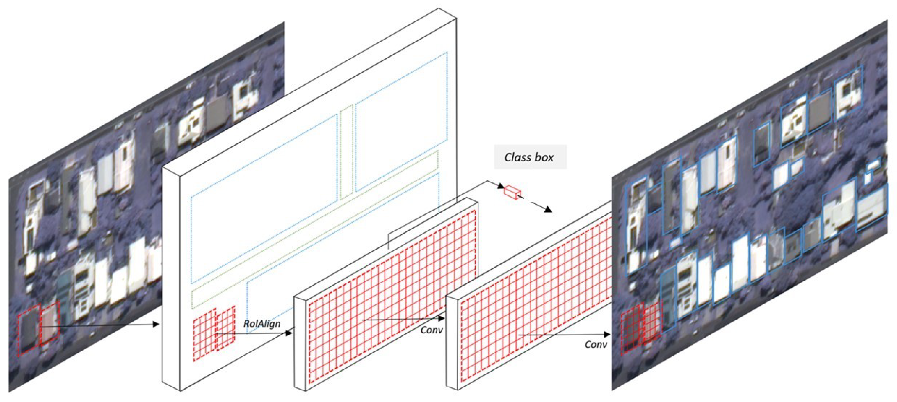
Detecting targets through remote sensing imagery using AI has been proven in the literature [8,9,10,14,15,16,18,19,20,21,22,23,24]. To contribute to the existing literature, this study utilised a progression of AI and machine learning (ML) called deep learning (DL) to automate the detection of ACM roofing through remote sensing imagery. Figure 2 shows the position of DL in the AI technology space. For the remainder of this study, the terminology DL will be used to represent the utilisation of this more sophisticated AI technique. This method of DL uses artificial neural networks (ANN) that are designed to replicate human learning processes more efficiently and beyond what ML is capable of [33]. ANN was enhanced to develop CNN, which is an efficient algorithm that can extract features by simultaneously using pixel classification and object detection to identify individual objects [33,34,35]. There are several enhancements between CNN and the Mask R-CNN used in this study. The predecessors of Mask R-CNN include a regional convolutional neural network (R-CNN) and Faster R-CNN. Mask R-CNN is currently the most evolved CNN algorithm with slightly enhanced architecture and the inclusion of a mask layer as an output [35]. Figure 3 provides a visualisation of the principle of Mask R-CNN. The architecture of Mask R-CNN processes images through a selected backbone to create abstract feature maps of the data. The feature maps are then scanned by the region proposal network (RPN) to identify potential objects [34,35]. Using region of interest alignment (RoIAlign) the model then extracts the features of the feature map according to the RPN. RoIAlign extracts the identified features without losing data like its predecessor region of interest pooling (RoIpooling) that is used in Faster R-CNN [33,34,35,36]. Two processes then occur using the extracted features. The model classifies the pixels of the identified objects, even if there are multiple classes, and the masks are generated for each class prediction, covering the extent of the object. This type of output is referred to as instance segmentation [37]. Further advantages of Mask R-CNN compared to other CNN methods is that it is easy to train, adaptable to other tasks and maintains efficiency with only a small increase in processing required compared to the Faster-R-CNN. In a 2022 survey by Bharati and Pramanik [35] that compared Mask R-CNN with other R-CNN methods, Mask R-CNN outperformed the other algorithms on an average precision of ~47.3%. Another 2022 study by Yu et al. [38] found that Mask R-CNN using remote sensing imageries achieved the highest accuracy when identifying individual trees (F1 = 94.68%) against other modelling algorithms, local maxima (F1 score = 87.68%) and marker-controlled watershed segmentation (F1 score = 85.92%).

1.5. Summary

This study progresses existing ACM detection research by leveraging from the advancements in remote sensing imagery and AI analytic methods. This study will investigate the use of Mask R-CNN to detect ACM roofing using HRAI and MSSI, as this has not yet been fully explored in the literature.

2. Methods

2.1. Overview

This section provides an overview of the method used for both the MSSI and HRAI models as visualised in Figure 4. The first step of the method was to identify a suitable case study area. The advice and observations of a subject matter expert (SME) was essential for establishing the case study area and creation of a training sample dataset of ACM roofing likelihood via desktop, observational analysis. Both types of imagery required input imagery preparation, training sample dataset creation, model training, and running the Mask R-CNN model and feedback loops. Variations occurred between the two models during the method process that resulted in different training sample datasets being used. To better discuss these variations, the model using HRAI and 460 training samples is hereon referred to as model 1, and the model using MSSI and 184 training samples is referred to as model 2. Finally, the results of ACM roofing detection were produced, analysed and discussed.
To further explore the effect of the variations on the results of models 1 and 2, a third model referred to as model 3 was produced. Model 3 used HRAI with a reduced training sample dataset to match that used in model 2 (184).

2.2. Case Study Area Selection

The first step of this research method is the case study area selection. To detect ACM in the residential built environment at a large scale, the process first requires the prediction of areas that have a higher occurrence of ACM anywhere in the building stock. This was achieved by understanding the socioeconomic and urban development characteristics of areas that had high development growth during the historical period of asbestos use and were also less likely to have been redeveloped since the ban in 2003. Using these characteristics, a multi-criteria analysis along with unsupervised cluster analysis was undertaken using the k-mean method. Results were reported spatially at a statistical area level 2s (SA2s) scale. Following the multi-criteria analysis and cluster analysis results, SA2s with the highest score were selected for further investigation. A preliminary investigation shortlisted 542 out of 2310 SA2s [39] across Australia. Further investigation resulted in the selection of six SA2s in Western Sydney, covering 26.8 km2, as an ideal case study area for this research.
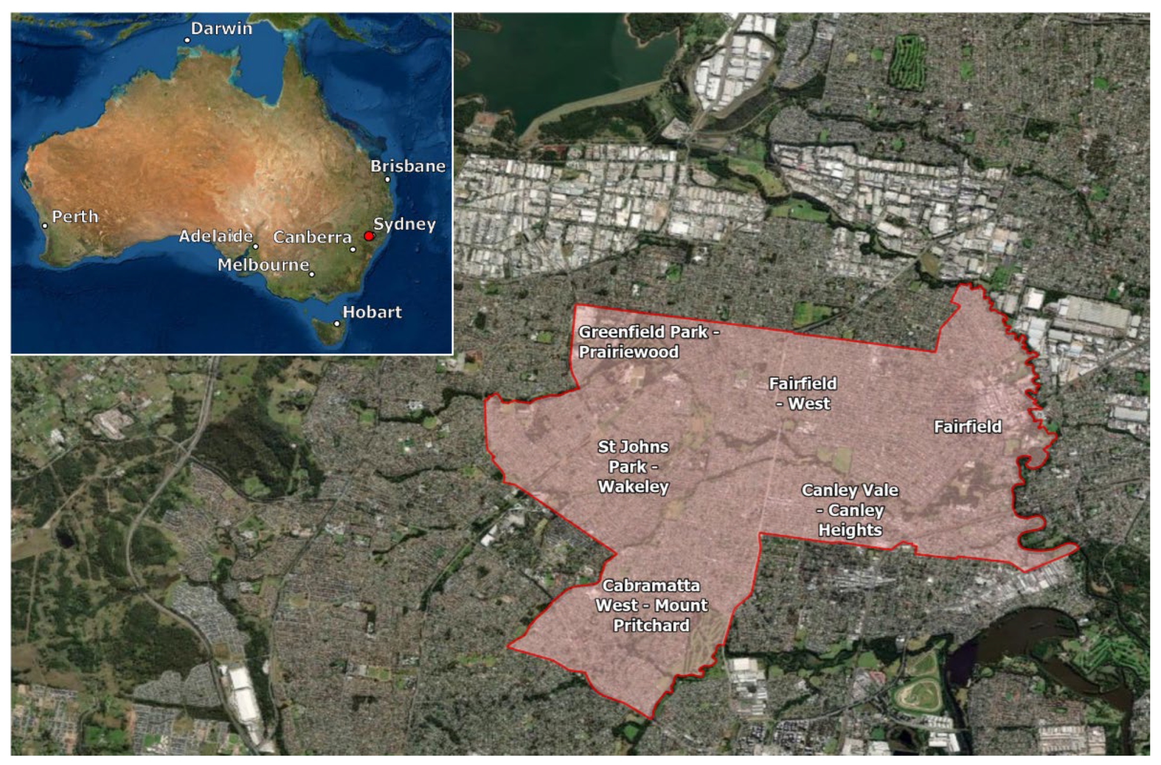
Western Sydney refers to a region of suburbs located to the west of the city of Sydney, New South Wales, Australia, as shown in Figure 5. Western Sydney began to grow in the late 1800s to 1900s as the opening of railway lines improved access to and from the dense city to the east [40]. Post-World War II, immigration, industrial growth and the construction of public housing estates dramatically increased the population in this region [40]. Residential development was occurring so rapidly that many building materials became expensive and inaccessible [41]. This increased the popularity of a cheaper and more accessible building material, fibrous cement sheeting (fibro-cement) [40]. From 1916 to 1983, a James Hardie asbestos manufacturing plant was operating in Parramatta, a suburb of Western Sydney [42]. This plant produced fibro-cement products containing asbestos, which were used heavily in the surrounding suburbs of Western Sydney and also distributed throughout Australia. As a result, Western Sydney forms part of Sydney’s “fibro-belt”, a term that refers to areas of greater Sydney with higher occurrences of fibro-cement housing [40,41]. Rapid expansion and redevelopment in this region are beginning to occur as the original building stocks are around 80 years old. The intense revitalisation fuelled by housing demand and investments seen in the inner suburbs of the city is not mirrored in the Western Sydney area, which had an average property market growth rate of 4.8% in the last two decades. In this area, redevelopment is occurring on a local, property-by-property scale, dispersed across the suburbs [40]. An observational desktop analysis was conducted to verify the prediction of the data that Western Sydney was an ideal case study area. This analysis used SME observations through aerial and street view imagery to present a likelihood of ACM in residential buildings in the area. The SME for this study was an occupational hygienist with over 25 years’ experience in asbestos and other hazardous materials surveying and land contamination assessment.

2.3. Input Imagery Data

The HRAI used for this study was 7.5-cm resolution RGB images purchased from a commercial aerial imagery producer and supplier. The MSSI was purchased from a commercial satellite imagery supplier that supplies imagery produced by the Worldview-3 satellite. The MSSI imagery included a 30-cm resolution panchromatic band (450–800 nm) and 1.24 m resolution multi-spectral bands (blue 450–510 nm, green 510–580 nm, red 655–690 nm, near infrared 780–920 nm, coastal and red-edge). The MSSI was processed using pan-sharpening to combine the high-resolution panchromatic raster dataset with a lower-resolution multiband raster dataset to create a high-resolution multiband raster dataset for remote sensing analysis. This approach creates high-resolution 8-band multi-spectral images that can be used to improve segmentation and classification. The MSSI had 0% cloud coverage and was within the 30 degrees off-nadir limit, which applies for the WorldView-3 satellite. Any variance in degrees off-nadir may change the way the multi-spectral signal interacts with the surface. The extent of variance and change in results was not measured as part of this study. Furthermore, the currencies of the imageries differ by a maximum of 6 months, the HRAI being more recently captured than the MSSI.

2.4. Training Sample Dataset Creation

Deep learning models were trained using examples of ACM roofing observed and extracted from HRAI and pan-sharpened MSSI. Figure 6 provides an overview of the input imagery search strategies, which involved analysts undertaking a systemic search of each SA2 in the case study area specifically for ACM roofing. Reference images of ACM roofing on residential dwellings were validated by an SME and provided to the analysts. Each analyst then undertook three search strategies across each SA2 from a desktop:
  • detailed aerial imagery searches scanning left to right across each urban block at different scales to identify different roofing materials depending on the imagery resolution,
  • a more distributed search strategy to scan across a broader area to better observe patterns of streets and property sizes at a larger scale,
  • ‘desktop-walking’ down the streets with ACM dwellings using Google Street-view to observe potential ACM roofing that could not be fully observed in aerial imagery.
During the searches, training samples were captured for the dataset by creating bounding boxes from approximately 0 to 1 m around the building footprint of the target dwelling. Depending on the variation of ACM roof types captured in the training samples, such as painted, unpainted, overall shape and area of the roof, further sampling was undertaken to improve representative sampling, reduce bias and enhance the model performance. The training sample dataset size could be increased from 184 using 30-cm MSSI for model 2, to 460 records using 7.5-cm HRAI for model 1. The higher resolution of the HRAI made it easier to observe the characteristics of ACM roofing, which increased target data detection and sampling. The training sample dataset for model 1 was not able to be applied to model 2 as the imageries had different currencies and aerial angles.
As model 1 and 2 have different-sized datasets, to further investigate the use of Mask R-CNN with MSSI and HRAI for the detection of ACM roofing, a third model was produced. Model 3 used HRAI; however, the training sample dataset for this model was limited to 184 samples to match the size of the dataset used for model 2. Furthermore, the 184 training samples were manually selected at random (with some consideration to representative sampling of different varieties of ACM roofing) from the 460 training samples used for model 1. Therefore, while the training sample dataset size matched for models 2 and 3, the geographical location of the training samples did not completely match due to the slight variation in imagery. All three training datasets were distributed across the case study area.

2.5. Model Training

The training sample dataset bounding boxes were used to produce image tiles (‘chips’) using the modelling software. The model training hyperparameters included the selection of tile sizes, which was set to 256 by 256 pixels around the training samples. These tiles were then used to train a deep learning model. Figure 7 provides a visual representation of the creation of the chips from the training samples.

2.6. Run Mask R-CNN Model

Table 3 summarises the process of the methods in this step. The geometric locational data created in the training dataset creation was used to produce the deep learning chips from the imagery. That chip data was then used to train the Mask R-CNN model.
The trained deep learning models were then processed using Mask R-CNN to detect ACM roofing within the case study area. The Mask R-CNN model required inputting the MSSI or HRAI for the relevant model that covered the case study area and the trained model. The number of epochs (i.e., number of times that the model loops through the data while training), learn rate (i.e., hyperparameter that defines how fast the model adapts to the target) and confidence threshold (set to 70–90%) were also calibrated for modelling optimisation. These hyperparameters were set according to parameters used in asbestos and non-asbestos detection literature that produced successful results. The chosen hyperparameter settings considered commentary from the literature that correlated certain hyperparameter adjustments to improved accuracy and precision. From there, manual adjustments were considered where required.

2.7. Feedback Loop

If the model inference accuracy was lower than 80%, true positives were incorporated to the training sample dataset to increase the sample size to improve the model performance. This would require using the inferences to identify roofs that could be added to the training sample dataset and re-running the model. The inference accuracy benchmark of 80% was selected as an industry-accepted benchmark of model output accuracy [10]. When considering the difference between using 70% or 90% as a benchmark for inference accuracy, there was minimal effect on the inference count regarding asbestos management.

3. Results

The following section outlines the results of the three models using MSSI and HRAI with Mask R-CNN to detect ACM roofing in the Australian residential building stock. The main results of this study are from model 1 and 2, followed by the results of model 3. Table 4 details the similarities and variabilities between models 1 and 2, including the case study area details and model parameters.
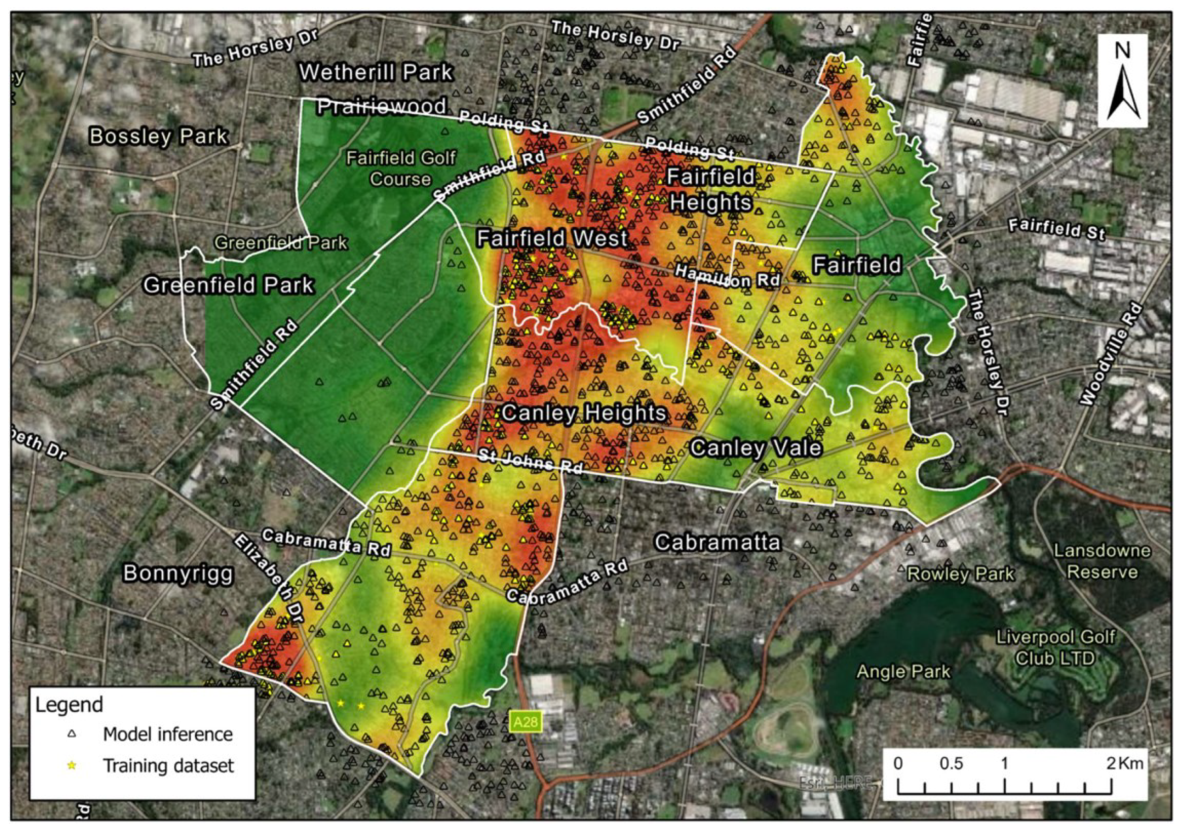
A residential asbestos heatmap for the Western Sydney area showing inference results produced by model 1, using 7.5-cm HRAI is illustrated in Figure 8.
A residential asbestos heatmap for the Western Sydney area showing inference results produced by model 2, using 30 cm MSSI is illustrated in Figure 9.
The distribution of the inferences across models 1 and 2 in Figure 8 and Figure 9, respectively, highlight similar areas where higher numbers of inferences were detected, in particular, Canfield Heights and Fairfield West areas. Furthermore, both figures have similar areas of scattered inferences, including Greenfield Park and the eastern area of Fairfield.
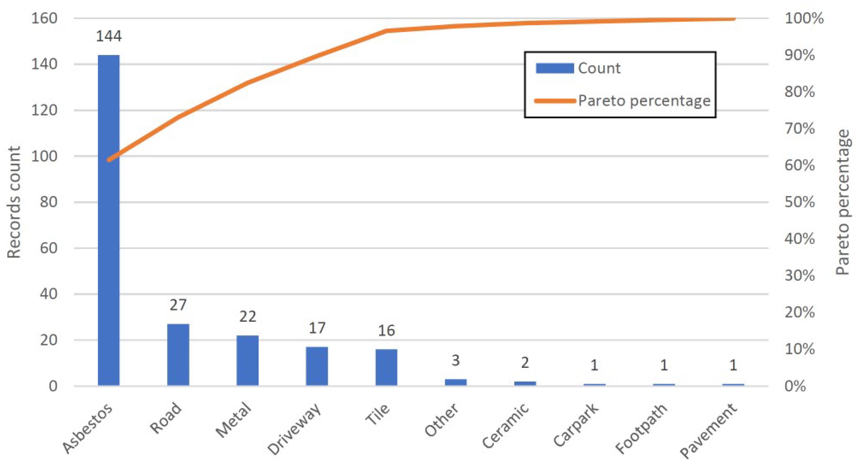
Using HRAI and Mask R-CNN, 1938 inferences of ACM roofing were detected with a 99.8% confidence threshold for model 1. The MSSI and Mask R-CNN model 2 detected 533 inferences of ACM roofing with a 90% confidence interval. The cut-off confidence interval threshold of the HRAI model was optimised to 99.8%. For this purpose, true and false positives and negatives within model 1 and the respective heatmap, asbestos clusters were considered, i.e., the Fairfield West asbestos cluster. In this cluster, a total of 234 records at a 50% confidence interval were identified and classified by the type of the actual material, as illustrated in Figure 10. This Pareto chart aids in defining the proportion of true and false positives for records. Out of 234 records detected as ACM roofing at 50% confidence, 144 inferences were ACM roofing and 90 were incorrect and post-identified as other materials, including tile, metal or pavement. Also included in Figure 10 is the cumulative Pareto percentage line, which shows the proportions as a percentage. In this measure, 62.5% of the inferences in the cluster were true positives and 37.5% were other materials and, therefore, false positives. The SME quality assurance using a stratified random sample of SA2s found four incorrect inferences out of 67 records, which is equivalent to 94% precision.
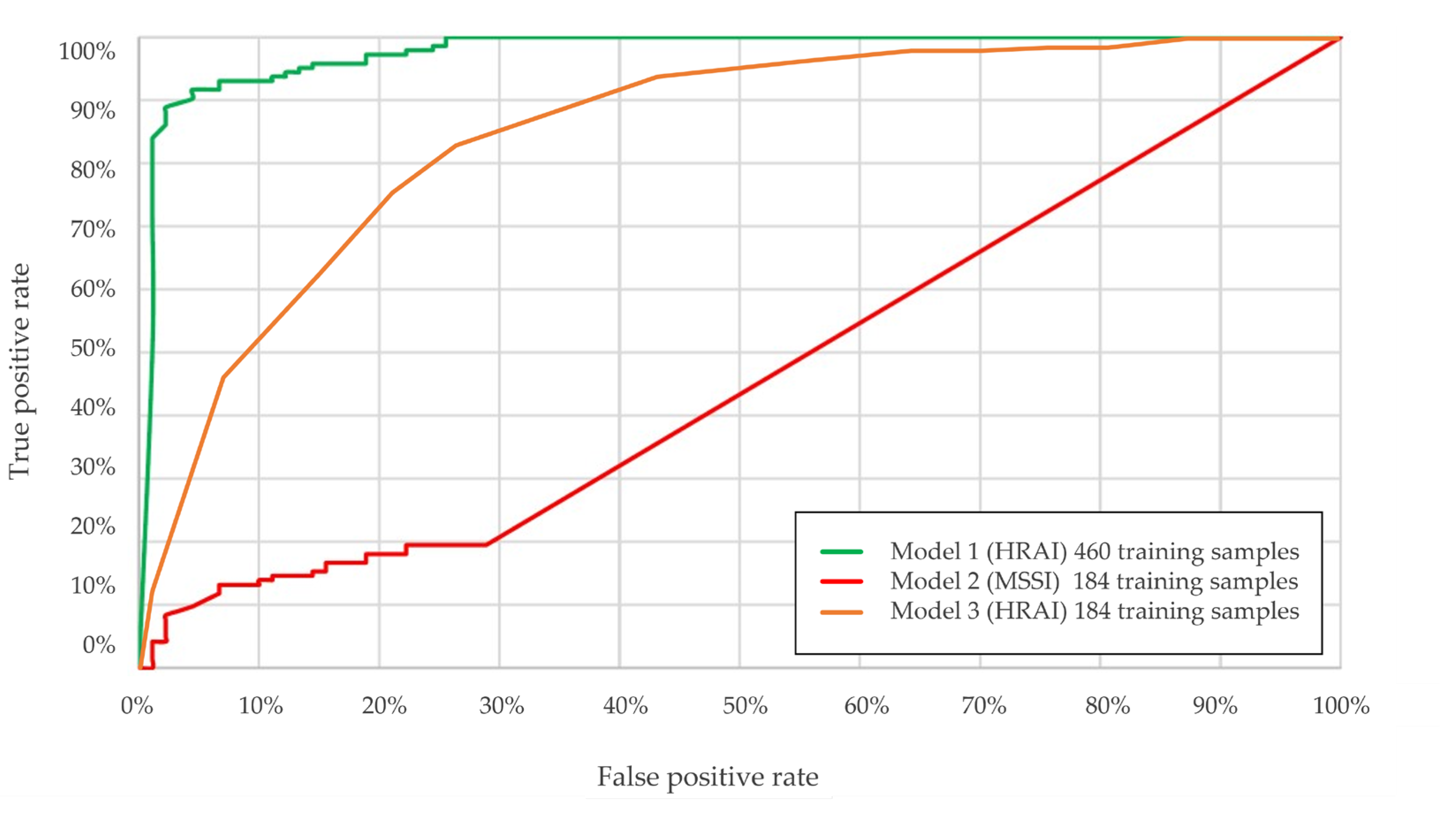
By also creating a receiver operator characteristic (ROC) curve for the Fairfield West asbestos cluster in Western Sydney, true positives (sensitivity) and false positives (specificity complement) were identified for different threshold values, as illustrated in Figure 11. This analysis provides a visual representation of the model accuracy, in which models with random precision follow a linear trend (i.e., true and false positives increase simultaneously). In this instance, this was the case with model 2. The low recall rate of model 2 resulted in reduced model precision. Models such as model 1 that sustain large true positive proportions (e.g., >80%) without a considerable increase in false positives are considered reliable models. Model 1 using HRAI had over 80% true positives with a small number of false positives. To avoid false positives in the records from model 1, the cut-off confidence interval threshold was set to 99.8%, totalling 1938 records across Western Sydney, as shown in Figure 8.
Furthermore, observations of the inferential results for models 1 and 2 saw that among the properties with ACM roofing detected, there was a large proportion of asbestos in outbuildings rather than the main dwelling. ACM roofing was also detected in several extensions to main buildings that have primarily tile roofs and a footprint of less than 100 m2. Such examples are indicative of pre-1950s properties with renovation undertaken during the asbestos era.
The ROC of the model 3 visualises its position of model performance in this study. It was not as precise or reliable as model 1 but still outperformed model 2 in those areas. While model 2 and 3 used the same sized training sample dataset and produced similar precision of 63% and 62% respectively, model 3 produced a larger number of inferences at a higher confidence threshold of 98%, as shown in Table 5.
Table 5 details the similarities and variabilities of the inputs, processing and outputs of models 2 and 3.

4. Discussion

The study results provide contributions across two key areas: (1) demonstration of the ability of Mask R-CNN models to detect ACM roofing, and in effect, the application of AI for improved asbestos management; (2) an investigation of modelling variables, assisting with decision making regarding the use of AI for ACM detection; and the considerations for model inputs, configuration, processing and outputs. Prior studies support the findings that there are many variables to consider for an optimal AI model [8,9,10,14,15,16,18,19,20,21,22,23,24]. Many trade-offs can be made throughout a study, customised for overall project management and technical execution requirements.
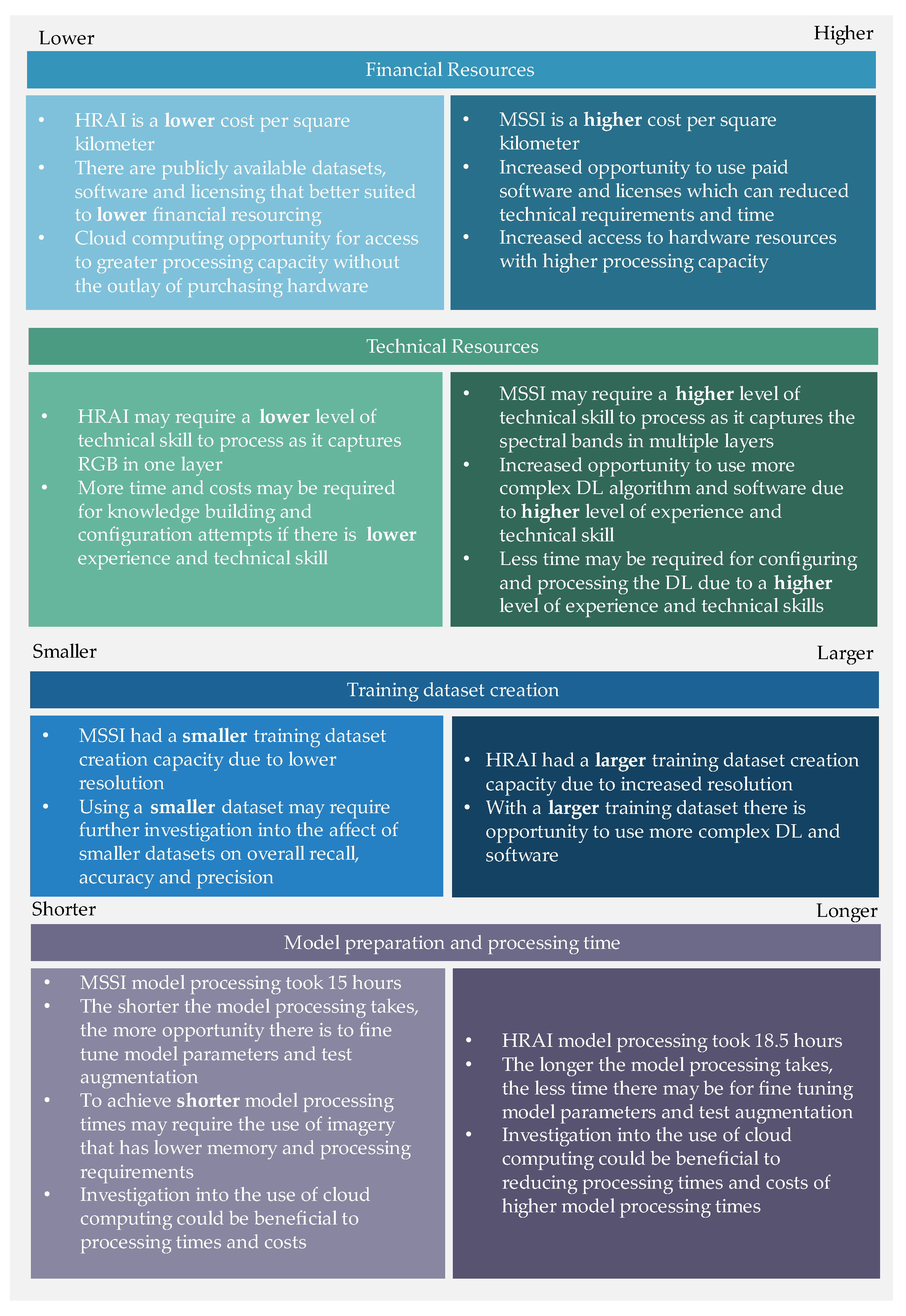
This study aimed to investigate the use of MSSI and HRAI to detect ACM roofing using Mask R-CNN. This was accomplished with some variations to each model that are important to explore to better understand current and future modelling outcomes. Previous publications [8,9,10,14,15,16,18,19,20,21,22,23,24] have shown that changing relationships between inputs, parameters and outputs can aid in understanding the efficiency and accuracy of a model. The following section discusses the detection of ACM roofing by Mask R-CNN and remote sensing imagery and the variables of this study that contributed to the configuration of the models. These variables include financial and technical resourcing, input data ownership and usage restrictions, input imagery types, training sample dataset creation, model preparation and processing times, and the application of DL. Figure 12 highlights the points of this discussion.

4.1. Financial and Technical Resources

For this study, model 2 used MSSI with 8 spectral bands with Mask R-CNN to accurately detect ACM roofing. However, model 1 using HRAI with 3 bands (RGB) with Mask R-CNN was also able to accurately detect ACM roofing and with greater precision. The ability to accurately detect ACM roofing with HRAI brings a potential cost reduction for future ACM roofing detection projects, as MSSI can be more expensive than high-resolution, RGB aerial imagery. Other costs to be considered for this study are relevant to machine hardware, modelling software, licensing for additional functions of the software and acquiring the modellers with the technical skills and experience required to achieve this study. This study required modellers with skills in GIS, DL and an in-depth understanding of ACM and its presentation in the urban environment. Workers with GIS and DL skillsets, with an overall background in computer and data science, and urban planning participated in every aspect of this study. SMEs with professional experience in occupational hygiene and asbestos, and other hazardous material surveying were brought into this project to provide their subject matter expertise at the inception of the project and the creation of the validation dataset.

4.2. Input Data Ownership and Usage Restrictions

For this study, limitations set by imagery suppliers required their permission to use DL analysis on the imagery. There were also limitations on outcomes and ownership of the derivative works produced by the analysis. These limitations were overcome for this study but imposed delays and additional costs to the project. Considering these types of data usage constraints at project commencement will assist with the successful delivery of the project. The ability to capture and procure public imagery and the increased availability of data from the rise in popularity of remote sensing imagery may reduce the impact of data ownership and usage restrictions in the future.

4.3. Input Imagery Characteristics

Coverage and currency: As detailed in Table 1, the accessibility of MSSI and HRAI can vary depending on the available extent of geographical coverage (coverage) and the timeliness of the data (currency). Coverage and currency can impede comparability, monitoring abilities and the timeframe of projects [25,26,27,28,29,30]. HRAI is more likely to be limited by currency and coverage due to the costs and accessibility of aerial vehicles and sensors for capturing; and it is not available for all settlements, particularly if they are outside metropolitan areas. MSSI is more accessible for coverage and currency as existing satellites with sensors can cover more area, more frequently. For this study, the same coverage was able to be sourced in both MSSI and HRAI due the metropolitan settlement of the case study area. The imageries had a maximum of a 6-month difference in currencies. The MSSI was 6 months older than the HRAI. ACM roofing captured in the MSSI model could have been redeveloped before the HRAI was captured, creating differences in inference results. However, since the average property market growth across the Western Sydney SA2s was 4.8% over the last two decades, redevelopment that occurred during that time potentially would not have impacted the inference results.
Spatial resolution: In a study by Bassani et al. [8], the pixel resolution of the HSSI and MSSI was a limitation for detecting smaller structures with ACM and mixed materials. This was not a limitation in this study as the results showed that all three models detected smaller areas of ACM roofing on smaller outbuildings and roof extensions. The Bassani et al. [16] study was completed in 2007 and used 3 m ground pixel resolution spectral satellite imagery, whereas this study used 30–1.24 m ground pixel resolution MSSI and 7.5 cm ground pixel HRAI. It is potentially the improved pixel resolution of the imageries used in this study that contributed to the increased detection of smaller ACM roofing structures.
Spectral resolution and signature: The presence of a spectral signature for ACM roofing detection is debated in the literature [9,10]. A study by Krówczyńska et al. [10] identified that HSSI, which has the highest spectral resolution compared to MSSI, was not necessary for detecting a spectral signature of ACM roofing. The study by Krówczyńska et al. [10] used multi-spectral aerial imagery containing RGB and colour-infrared spectral bands and identified that when using CNNs, the spectral resolution only affected the classification accuracy by 2%. Furthermore, the accurate capture of spectral bands can vary depending on numerous environmental factors, including topography and roofing typology, which is relevant for studies using wide-scale coverage of the built environment. In a study using HSSI, Frassy et al. [18] found the mountainous typology of the study area did not affect the study results. However, in a study by Fiumi, Congedo and Meoni [43], also using HSSI, the vaulted and pitched roofing typology did affect the study results. The presence of a spectral signature or the effect the environmental factors had on the spectral resolution of the MSSI in this study was not investigated. If the presence of a spectral signature or environmental factors did influence the model 2 results by using MSSI, the impact was potentially minimal, as evident in Krówczyńska et al. [10].

4.4. Training Sample Dataset Creation and Size

One of the main challenges during the research development was that there were no pre-existing training sample datasets for ACM roofing to train DL models. Therefore, new data needed to be created. The creation of the training sample dataset utilised the expertise of the SME to observationally identify ACM roofing using the HRAI and MSSI imagery. The spatial resolution of the imagery was an influencing factor in the number of training samples that could be identified. The characteristics of ACM roofing were easily observed in the HRAI compared to MSSI; and as a result, more training samples were captured for model 1. The increased training samples for model 1 increased the recall results, increasing the overall performance of that model. The training sample dataset created using HRAI could not be used for model 2 due to the difference in currency between the imageries and an approximately 2-m difference in aerial angle that created a minor spatial difference between the imageries. Model 1 using HRAI and 460 training samples produced 1938 inferences at a precision of 94% and a 99.8% confidence threshold. Model 2 using MSSI and 184 training samples produced 533 inferences at 63% precision and a 90% confidence threshold. Model 3 using HRAI and 184 training samples produced 1737 inferences at 62% precision and a 97% confidence threshold. The literature presents results showing a minimal reduction in overall performance using varying training sample sizes [44,45,46]. For example, a study by Xu et al. [44] for crack detecting using Faster R-CNN and Mask R-CNN achieved sufficiently accurate results using only 130+ training samples. Furthermore, a land cover study by Ramezan et al. [46] that compared machine-learning algorithm accuracy when applied to large and small datasets identified only a 1% decrease in accuracy between the two when applying a Random Forest model. While these studies were successful using small datasets to detect their objectives, this was not consistent with the findings of this study for ACM roofing. From this study, the ROCs of the three models indicate that the model with the larger training sample dataset, model 1, was the more reliable model, and its precision and recall rating supported that. The ROCs of models 2 and 3 illustrate a lower model performance and reliability, which is potentially correlated to the training dataset size. To detect ACM roofing using smaller dataset efficiently and precisely, this would require further model alterations and research.

4.5. Model Preparation and Processing Time

The preparation of the input data and model configuration involved identifying compatibility between software and imageries, ordering and addressing limitations of use with the imagery, working with SMEs to understand what ACM in the built environment looks like, the creation of the training sample dataset, understanding the DL model requirements, and configuring the model hyperparameters. The initial manual input required for DL modelling is necessary to begin to reduce the amount of manual input required. For example, creating 460 training samples produced 1938 inferences of ACM roofing at a high precision and confidence. During upscaling, the validated inferences can be used to increase the training sample dataset and, therefore, the automated processing gains momentum, lowering the workload and increasing production of inferences even further. This momentum could not occur through the traditional methods of ACM identification as the nature of the process presents one result to one sample.
Models 1 and 2 were processed using Mask R-CNN to produce inferences in a time of 18.5 h and 15 h, respectively. Model 3 processed in a time of 10 h. The models were processed separately on the same machine using the local 16 GB random access memory (RAM), graphic processing unit (GPU), software and libraries. The variations in the training sample datasets sizes, spectral and spatial resolutions are potentially the cause of the variation in processing time. The overall processing time of the models can be attributed to the format size of the imageries used. Both imageries were supplied, processed and stored in georeferenced tagged image file format. A georeferenced tagged image file format is a data-heavy format that requires more memory for storing and processing when compared to a portable network graphic format. Upscaling this study beyond 26.8 km2 would increase the size of the imagery required. To keep processing times within an efficient timeframe, greater processing capacity may be required. There are financial, accessibility and technological limitations related to upgrading the necessary hardware, software and licenses to accommodate the upscaling of large data projects [42]. An option to avoid these limitations while being able to progress with upscaling is cloud computing. Cloud computing is a concept that is becoming more prominent in the DL space, in place of traditional technological upgrades [47], as it can provide on-demand agility in data storage, processing capacity, timeframes and costs. Accessing virtual storage and processing capacity opens the opportunities for upscaling into large data projects with more timely processing.

4.6. Application of Deep Learning

As found by Guo et al. [14] and Zhang et al. [15], advancements in deep learning have provided opportunities to improve object detection, therefore improving the ability to detect ACM roofing. This was evident in this study as the current evolution of AI-based segmentation algorithms, i.e., Mask R-CNN, successfully detected ACM roofing. This is also proven in a study by Iqbal et al. [23] that tested Mask R-CNN and previous versions of CNNs to detect individual trees. In that study, Mask R-CNN outperformed the previous versions with a classification accuracy of 96–98% [23]. In this study, model 1 had a higher precision of 94% when using Mask R-CNN. Models 2 and 3 had a similar precision, with 63% for model 2 and 62% for model 3. The model 3 ROC showed it was a better performing model. Model 3 produced more inferences at a similar precision to model 2, potentially due to the higher resolution of the imagery. Results seen in a study by Weih and Riggan [17] also highlighted the increase in accuracy of object detection methods when using HRAI, compared with MSSI. This is potentially due to the object detection algorithm addition that is used by Mask R-CNN to achieve instance segmentation [17]. As artificial intelligence and descendant algorithms improve, other algorithms could replicate the results of this study or improve upon them with the correct application.

5. Conclusions

This study investigated the use of AI, specifically Mask R-CNN, to detect ACM roofing using HRAI and MSSI in a case study area in Australia. Model 1 using HRAI and 460 training samples produced 1938 inferences at a precision of 94% and a 99.8% confidence threshold. Model 2 using MSSI and 184 training samples produced 533 inferences at 63% precision and a 90% confidence threshold. Model 3 using HRAI and 184 training samples produced 1737 inferences at 62% precision and a 97% confidence threshold. The results across the three models indicate that model 1, using HRAI and a larger training sample dataset with Mask R-CNN, produced the highest number of inferences at the highest precision and confidence threshold. Overall, this study confirmed the efficacy of AI (i.e., Mask RCNN) to detect ACM roofing using remote sensing imagery. Without replacing traditional in situ inspection and detection methods, AI detection methods can be useful to widen the scale of investigation coverage and better allocate resources for targeted investigations in areas that have a high likelihood for asbestos. Wide-scale AI detection of ACM roofing can provide a foundation for cost-effective larger-scale detection of asbestos roofing. The cost-effective techniques described in this paper can be applied by governments and stakeholders for the safe management and disposal of ACM in developed, developing and undeveloped regions worldwide.

6. Future Research Direction

The application of AI in ACM detection is being recognised for its benefits [9,10,14,15,16,18,19] in introducing newer available resources to assist with addressing this global problem. For example, cloud computing, automated training, publicly available imagery databases, UAV technology and open-source coding libraries are all recent innovations that assist with improved detection of ACM roofing using AI. These innovations contribute to improving the efficiency of financial and technical resourcing, input data ownership and usage restrictions, the use of input imagery types, training sample dataset creation, model preparation and processing times, and the application of DL.
As part of this study, a total training sample of 648 records was created for Western Sydney, which can be increased to over 2400 records by using inferential model results in future upscaled studies. Increasing the training sample dataset using high-resolution imagery over other areas during the upscale may also improve the model accuracy by increasing the training sample dataset variability [43,44].
Investigations to further understand the effect of geography and roofing typology on spectral signatures when using MSSI with Mask R-CNN could aid in reducing any potential impact of spectral signature on the overall recall rate. More to this point, the case study area overall had some variation in geography and roofing typology; however, upscaling this study to areas with greater variation in these aspects would require more representative sampling for HRAI in addition to spectral signature investigation. Furthermore, the reproduction or upscaling of this study should consider utilising the processing power of cloud computing to reduce the timeframe for model processing and decrease the overall costs associated with this aspect of the study.
Finally, if the currency of HRAI and MSSI can be matched, a larger training sample dataset can be created using HRAI and then transferred to MSSI to allow for the full performance capability of an MSSI-based, Mask R-CNN ACM detection model to be known.

Author Contributions

Conceptualisation, M.V.H., N.P., R.A.S., A.S.V. and G.F.K.; methodology, M.V.H., N.P., R.A.S., A.S.V. and G.F.K.; validation, M.V.H., N.P. and A.S.V.; investigation, M.V.H., N.P. and A.S.V.; data curation, M.V.H., N.P. and A.S.V.; writing—original draft preparation, M.V.H., N.P. and A.S.V.; writing—review and editing, M.V.H., N.P., R.A.S., A.S.V. and G.F.K.; visualisation, M.V.H.; supervision, N.P., R.A.S. and A.S.V. All authors have read and agreed to the published version of the manuscript.

Funding

This paper is part of a Griffith University Postgraduate Research Scholarship sponsored by Griffith University, Southport, Australia and UACS Consulting Pty Ltd., Buderim, Australia. The study of the paper commenced with the support of two projects contracted by and in conjunction with the Australian Federal Government branch, Asbestos Safety and Eradication Agency.

Funding

This paper is part of a Griffith University Postgraduate Research Scholarship sponsored by Griffith University, Southport, Australia and UACS Consulting Pty Ltd., Buderim, Australia. The study of the paper commenced with the support of two projects contracted by and in conjunction with the Australian Government Asbestos Safety and Eradication Agency.

Institutional Review Board Statement

Not applicable.

Informed Consent Statement

Not applicable.

Data Availability Statement

Restrictions apply to the availability of these data.

Conflicts of Interest

The research is part of a research program with Griffith, UACS and ASEA, including the authorship of this paper. The research program is collaboratively funded by all partners, which were involved in the choice of the research, design of the study, writing of the manuscript and decision to publish the results.

References

  1. Furuya, S.; Chimed-Ochir, O.; Takahashi, K.; David, A.; Takala, J. Global asbestos disaster. Int. J. Environ. Res. Public Health 2018, 15, 1000. [Google Scholar] [CrossRef] [PubMed] [Green Version]
  2. Frank, A. Global use of asbestos—Legitimate and illegitimate issues. J. Occup. Med. Toxicol. 2020, 15, 16. [Google Scholar] [CrossRef] [PubMed]
  3. International Agency for Research on Cancer (IARC). Arsenic, Metals, Fibres, and Dusts—Volume 100C Asbestos (Chrysotile, Amosite, Crocidolite, Tremolite, Actinolite, and Anthophyllite), in IARC Monographs on the Evaluation of Carcinogenic Risks to Humans. Available online: https://publications.iarc.fr/120 (accessed on 20 May 2022).
  4. Asbestos Safety and Eradication Agency (ASEA). National Asbestos Profile of Australia. 2017. Available online: https://www.asbestossafety.gov.au/sites/default/files/documents/2017-12/ASEA_National_Asbestos_Profile_interactive_Nov17.pdf (accessed on 11 May 2022).
  5. Asbestos Safety and Eradication Agency. Updated Asbestos Stocks and Flows Model. Available online: https://www.asbestossafety.gov.au/what-we-do/news-and-announcements/updated-asbestos-stocks-and-flows-model (accessed on 26 July 2022).
  6. Institute for Health Metrics and Evaluation. Global Burden of Disease (GBD). 2019. Available online: https://www.healthdata.org/gbd/gbd-2019-resources (accessed on 11 May 2022).
  7. Brown, B.; Hollins, I.; Pickin, J.; Donovan, S. Asbestos Stocks and Flows Legacy in Australia. Sustainability 2023, 15, 2282. [Google Scholar] [CrossRef]
  8. Abbasi, M.; Mostafa, S.; Vieira, A.S.; Patorniti, N.; Stewart, R.A. Mapping Roofing with Asbestos-Containing Material by Using Remote Sensing Imagery and Machine Learning-Based Image Classification: A State-of-the-Art Review. Sustainability 2022, 14, 8068. [Google Scholar] [CrossRef]
  9. Tommasini, M.; Bacciottini, A.; Gherardelli, M. A QGIS Tool for Automatically Identifying Asbestos Roofing. ISPRS Int. J. Geo-Inf. 2019, 8, 131. [Google Scholar] [CrossRef] [Green Version]
  10. Krówczyńska, M.; Raczko, E.; Staniszewska, N.; Wilk, E. Asbestos-cement roofing identification using remote sensing and convolutional neural networks (CNNs). Remote Sens. 2020, 12, 408. [Google Scholar] [CrossRef] [Green Version]
  11. Safe Work Australia. Model Work Health and Safety Regulations 2011, updated January 2021. Available online: https://www.safeworkaustralia.gov.au/doc/model-whs-regulations (accessed on 1 November 2022).
  12. Asbestos Safety and Eradication Agency. Asbestos in the Home. Available online: https://www.asbestossafety.gov.au/find-out-about-asbestos/asbestos-home (accessed on 11 May 2022).
  13. AS 4964-2004; Method for the Qualitative Identification of Asbestos in Bulk Samples. Standards Australia: Sydney, Australia, 2004. Available online: https://www.standards.org.au/standards-catalogue/sa-snz/other/ch-031/as-4964-2004 (accessed on 1 November 2022).
  14. Guo, W.; Yang, W.; Zhang, H.; Hua, G. Geospatial Object Detection in High-resolution Satellite Images Based on Multi-Scale Convolutional Neural Network. Remote Sens. 2018, 10, 131. [Google Scholar] [CrossRef] [Green Version]
  15. Zhang, L.; Zhang, L.; Du, B. Deep Learning for Remote Sensing Data. IEEE Xplore 2016, 4, 22–40. [Google Scholar]
  16. Bassani, C.; Maria, R.; Cavalcante, F.; Cuomo, V.; Palombo, A.; Pascucci, S.; Pignatti, S. Deterioration status of asbestos-cement roofing sheets assessed by analysing hyperspectral data. Remote Sens. 2017, 109, 361–378. [Google Scholar]
  17. Weih, R.C.; Riggan, N.D. Object-based classification vs. pixel-based classification: Comparative importance of multi-resolution imagery. ISPRS J. Photogramm. Remote Sens. 2008, 38, C7. [Google Scholar]
  18. Frassy, F.; Candiani, G.; Rusmini, M.; Maianti, P.; Marchesi, A.; Nodari, F.R.; Via, G.D.; Albonico, C.; Gianinetto, M. Mapping asbestos-cement roofing with hyperspectral remote sensing over a large mountain region of the Italian western alps. Sensors 2014, 14, 15900–15913. [Google Scholar] [CrossRef] [PubMed] [Green Version]
  19. Taherzadeh, E.; Shafri, H.Z.M. Development of a generic model for the detection of roof materials based on an object-based approach using WorldView-2 satellite imagery. Adv. Remote Sens. 2013, 2, 312–321. [Google Scholar] [CrossRef] [Green Version]
  20. Toth, C.; Jóźków, G. Remote sensing platforms and sensors: A survey. ISPRS J. Photogramm. Remote Sens. 2016, 115, 22–36. [Google Scholar] [CrossRef]
  21. Houborg, R.; Fisher, J.; Skidmore, A. Advances in remote sensing of vegetation function and traits. Int. J. App. Earth Obs. Geoinform. 2015, 43, 1–6. [Google Scholar] [CrossRef] [Green Version]
  22. Sarker, I. AI-Based Modeling: Techniques, Applications and Research Issues towards Automation, Intelligent and Smart Systems. SN Comput. Sci. 2022, 3, 158. [Google Scholar] [CrossRef]
  23. Iqbal, M.; Ali, H.; Tran, S.; Iqbal, T. Coconut trees detection and segmentation in aerial imagery using mask region-based convolution neural network. IET Comp. Vis. 2021, 15, 428–439. [Google Scholar] [CrossRef]
  24. Campbell, J.; Wynne, R. Introduction to Remote Sensing, 5th ed.; The Guildford Press: New York, NY, USA, 2011. [Google Scholar]
  25. Aerometrex. Key Factors to Consider When Choosing between Aerial and Satellite Imagery. Available online: https://aerometrex.com.au/resources/blog/key-factors-consider-when-choosing-between-aerial-satellite-imagery/ (accessed on 20 May 2022).
  26. Ose, K.; Corpetti, T.; Demagistri, L. Multispectral satellite image processing. In Optical Remote Sensing of Land Surface; Elsevier: Amsterdam, The Netherlands, 2016; pp. 57–124. [Google Scholar] [CrossRef]
  27. Apollo Mapping. High Resolution Satellite & Aerial Imagery. Available online: https://apollomapping.com/imagery/high-resolution-imagery (accessed on 21 May 2022).
  28. Digital Globe. Worldview-3. Available online: http://content.satimagingcorp.com.s3.amazonaws.com/media/pdf/WorldView-3-PDF-Download.pdf (accessed on 21 May 2022).
  29. Aerometrex. The Company. Available online: https://aerometrex.com.au/about/company/ (accessed on 2 August 2022).
  30. Nearmap. Current Aerial Maps Average. Available online: https://www.nearmap.com/au/en/current-aerial-maps-coverage (accessed on 2 August 2022).
  31. American Association for the Advancement of Science (AAAS). High Resolution Satellite Imagery Ordering and Analysis Handbook. Available online: https://www.aaas.org/resources/high-resolution-satellite-imagery-ordering-and-analysis-handbook (accessed on 20 May 2022).
  32. Harvey, M.; Pearson, S.; Alexander, K.; Rowland, J.; White, P. Unmanned aerial vehicles (UAV) for cost effective aerial orthophotos and digital surface models (DSM). In Proceedings of the New Zealand Geothermal Workshop, Auckland, New Zealand, 24–26 November 2014. [Google Scholar]
  33. Sarker, I. Deep Learning: A Comprehensive Overview on Techniques, Taxonomy, Applications and Research Directions. SN Comput. Sci. 2021, 2, 420. [Google Scholar] [CrossRef]
  34. Wang, D.; Liu, Z.; Gu, X.; Wu, W.; Chen, Y.; Wang, L. Automatic Detection of Pothole Distress in Asphalt Pavement Using Improved Convolutional Neural Networks. Remote Sens. 2022, 14, 3892. [Google Scholar] [CrossRef]
  35. Bharati, P.; Pramanik, A. Deep Learning Techniques—R-CNN to Mask R-CNN: A Survey. In Computational Intelligence in Pattern Recognition; Das, A., Nayak, J., Naik, B., Pati, S., Pelusi, D., Eds.; Springer: Singapore, 2019; Volume 999, pp. 657–668. [Google Scholar]
  36. Khanzode, C.A.; Sarode, R.D. Advantages and Disadvantages of Artificial Intelligence and Machine Learning: A Literature Review. Int. J. Lib. Inform. Sci. 2020, 9, 30–36. [Google Scholar]
  37. Hafiz, A.M.; Bhat, G.M. A survey on instance segmentation: State of the art. Int. J. Multimed. Inf. Retr. 2020, 9, 171–189. [Google Scholar] [CrossRef]
  38. Yu, K.; Hao, Z.; Post, C.J.; Mikhailova, E.A.; Lin, L.; Zhao, G.; Tian, S. Comparison of Classical Methods and Mask R-CNN for Automatic Tree Detection and Mapping Using UAV Imagery. Remote Sens. 2022, 14, 295. [Google Scholar] [CrossRef]
  39. 1270.0.55.001; Australian Statistical Geography Standard (ASGS): Volume 1—Main Structure and Greater Capital City Statistical Areas. Australia Bureau of Statistics: Canberra, Australia, 2016. Available online: https://www.abs.gov.au/ausstats/[email protected]/lookup/by%20subject/1270.0.55.001~july%202016~main%20features~statistical%20area%20level%202%20(sa2)~10014#:~:text=Their%20purpose%20is%20to%20represent,Australia%20without%20gaps%20or%20overlaps (accessed on 2 December 2021).
  40. Pinnegar, S.; Freestone, R.; Randolph, B. Suburban reinvestment through ‘knockdown rebuild’ in Sydney. In Suburbanization in Global Society (Research in Urban Sociology); Clapson, M., Hutchison, R., Eds.; Emerald Group Publishing Limited: Bingley, UK, 2010; pp. 205–229. [Google Scholar]
  41. Australia Bureau of Statistics Search Census Data. Available online: https://www.abs.gov.au/census/find-census-data/search-by-area (accessed on 2 December 2021).
  42. Gwyther, G. From Cowpastures to pigs’ heads: The development and character of western Sydney. Sydney J. 2008, 1, 51–74. [Google Scholar] [CrossRef] [Green Version]
  43. Fiumi, L.; Congedo, L.; Meoni, C. Developing expeditious methodology for mapping asbestos-cement roof coverings over the territory of Lazio Region. App. Geomat. 2014, 6, 37–48. [Google Scholar] [CrossRef]
  44. Xu, X.; Zhao, M.; Shi, P.; Ren, R.; He, X.; Wei, X.; Yang, H. Crack Detection and Comparison Study Based on Faster R-CNN and Mask R-CNN. Sensors 2022, 22, 1215. [Google Scholar] [CrossRef]
  45. Ramezan, C.A.; Warner, T.A.; Maxwell, A.E.; Price, B.S. Effects of Training Set Size on Supervised Machine-Learning Land-Cover Classification of Large-Area High-Resolution Remotely Sensed Data. Remote Sens. 2021, 13, 368. [Google Scholar] [CrossRef]
  46. Liu, Y.; Liu, J.; Pu, H.; Liu, Y.; Song, S. Instance Segmentation of Outdoor Sports Ground from High Spatial Resolution Remote Sensing Imagery Using the Improved Mask R-CNN. Int. J. Geosci. 2019, 10, 884–905. [Google Scholar] [CrossRef] [Green Version]
  47. Velásquez, N.; Estévez, E.C.; Pesado, P.M. Cloud computing, big data and the industry 4.0 reference architectures. J. Comp. Sci. Tech. 2018, 18, 258–266. [Google Scholar] [CrossRef]
Figure 1. Visual comparison of HRAI 3 bands and MSSI 8 bands.
Sustainability 15 04276 g001
Figure 2. Overview of the progression of artificial intelligence to deep learning and the evolution to mask region-based convolutional neural networks.
Sustainability 15 04276 g002
Figure 3. Mask region-based convolutional neural network principle.
Sustainability 15 04276 g003
Figure 4. Study method overview.
Sustainability 15 04276 g004
Figure 5. Western Sydney case study area.
Sustainability 15 04276 g005
Figure 6. Overview of imagery search strategies for the training sample dataset creation.
Sustainability 15 04276 g006
Figure 7. Overview of masking training samples and tile creation.
Sustainability 15 04276 g007
Figure 8. Western Sydney case study area residential ACM roofing heatmap produced by model 1.
Sustainability 15 04276 g008
Figure 9. Western Sydney case study area residential ACM roofing heatmap produced by model 2.
Sustainability 15 04276 g009
Figure 10. Model 1 inferences at 50% confidence interval for Fairfield West asbestos cluster in Western Sydney case study area.
Sustainability 15 04276 g010
Figure 11. ROC curves for models 1, 2 and 3.
Sustainability 15 04276 g011
Figure 12. Summary of variables to consider for this study.
Sustainability 15 04276 g012
Table 1. Comparison of MSSI and HRAI attributes.
AttributesMSSIHRAI
Method of captureSeveral photos of the same scene using different sensors attached to a satellite (see Figure 1B,D) [25]. One photo taken of one scene until the desired area is covered using a high-resolution camera attached to an aerial vehicle (see Figure 1A,C) [24].
Bands of the electromagnetic spectrum capturedApproximately 3 to 10 bands depending on the number of sensors. Bands can include red, green, blue (RGB), near-infrared, thermal infrared, short-wave infrared, panchromatic, cirrus and thermal infrared [26]Three bands available: red, green, blue (RGB).
Available resolutionThree to four types of resolution are generally available.
  • low resolution: over 60 m per pixel,
  • medium resolution: 10–30 m per pixel,
  • high to very high resolution: 0.3–5 m per pixel [25,27].
High to very high-resolution available ranging from 2.5 to 10–15 cm per pixel [25,27]
WeatherGenerally, cannot guarantee cloud-free imagery, particularly over tropical areas. MSSI can be affected by atmospheric interference, which requires post-processing corrections [25].Flexible data capturing subject to the local weather, including altitude adjustments. This can guarantee cloud-free data and aerial imagery is not impacted by atmospheric interference [25].
Location accuracy and accessibilityGeneral accuracy is 10–20 m without ground control points, and accuracy is improving with new satellite technology [25].General horizontal accuracy is two pixels and the accuracy of aerial imagery is improving with the use of airborne ground positioning systems and post-processing.
SpeedGenerally, capturing specific locations and time-sensitive events cannot be guaranteed within two to three days, as they are depending on the satellite’s position in orbit. Worldview-3 has an average revisit time of less than one day [28]. MSSI processing times are low as there is usually a smaller number of images to process due to the coverage. HRAI is useful for specific locations or time-sensitive events depending on the availability of the equipment to the location. Processing times for this imagery are dependent on the number of images captured for coverage. This is improving with advancements in technology [25].
Coverage and currencyMSSI can quickly cover large geographic areas when in the correct place. Worldview-3 can cover up to 680,000 km2 per day [28].HRAI can capture large amounts of data in a small quantity of data collection runs. Commercial aerial imagery providers in Australia update the coverage of metropolitan areas 2–6 times a year and can provide access up to 3900 to 130,100 per km2 [29,30].
CostVaries depending on resolutions, accuracy and timeliness. Worldview-1 and Worldview-2 cost anywhere between AUD$14 1 and AUD$23 1 per km2 depending on the currency [27,31]Varies depending on mobilisation costs, resolution, accuracy, timeliness and if manned or unmanned [25]. Commercial suppliers can charge AUD$5.91 1 per km2 for 15 cm resolution, archived, orthorectified, aerial imagery captured by a manned aerial vehicle [27]. Unmanned aerial vehicles (UAV) capture, such as using drones, can lower associated costs [32].
1 AUD$1 = USD$0.67 November 2022.
Table 2. Reported remote sensing imagery studies including ACM-related studies.
AuthorResolution (Metres)BandsCapture
Weih and Riggan (2008) [17] 1 m11Aerial & satellite
1 m7Aerial & satellite
10 m8Satellite
Bassani et al. (2007) * [16]3 m102 (hyperspectral)Aerial
Frassy et al. (2014) * [18]4 m102 (hyperspectral)Aerial
6 m–9 m102 (hyperspectral)Aerial
Taherzadeh and Shafri (2013) * [19]0.5 m8 (visible and near-infrared)Satellite
Guo et al. (2018) [14]0.5 m–2 m3 (RGB)Satellite
0.08 m2 (colour-infrared)Satellite
Krówczyńska et al. (2020) * [10]0.25 m5 (RBG & colour-infrared)Aerial
* ACM roofing related.
Table 3. Summary of data created prior to Mask R-CNN model run.
MethodFormatModelData Created
Training Dataset Creation
Used SME observations, desktop analysis and imagery to outline potential ACM roofing locations Polygon shapefile Model 1460 polygons of ACM roofing locations
Model 2184 polygons of ACM roofing locations
Model 3184 polygons of ACM roofing locations
Model training
Created ‘chips’ of imagery from the locations of the training dataset creation step and used them to train the model.Tag Image Film Format (TIFF)Model 1HRAI 7.5 cm resolution chips of ACM roofs
Model 2MSSI 30 cm resolution chips of ACM roofs
Model 3HRAI 7.5 cm resolution chips of ACM roofs
Table 4. Model 1 and 2 similarities and variabilities.
Model ParametersModel 1—HRAIModel 2—MSSI
Case Study Area Details
AreaWestern Sydney Western Sydney
Included SA2sCabramatta West—Mount Prichard, Canley Vale—Canley Heights, Fairfield, Fairfield—West, Greenfield Park—Prairiewood, St. Johns Park—Wakeley Cabramatta West—Mount Prichard, Canley Vale—Canley Heights, Fairfield, Fairfield—West, Greenfield Park—Prairiewood, St. Johns Park—Wakeley
Population (2016) [41]93,94493,944
Dwelling Count (2016) [41]29,59529,595
Area (km2) (2016) [41]26.826.8
Model input
Model typeMask R-CNNMask R-CNN
Training sample size460184
Input imagery resolution7.5 cm30 cm & 1.24 m
Input imagery band types3 (RGB)8 (RGB, red-edge, coastal, near-infrared 1, near-infrared 2 & panchromatic)
Input imagery pre-processingN/APan-sharpening
Model processing
Processing unitGraphics processing unit (GPU)Graphics processing unit (GPU)
Processing time15 h18 h 30 min
Model output
Confidence threshold99.8%90%
Recall rate (inferences)1938533
Average precision94%63%
Table 5. Comparison of MSSI and HRAI (smaller training sample dataset) inputs and outputs.
Model ParametersModel 2—MSSI Model 3—HRAI
Model Input
Model typeMask R-CNNMask R-CNN
Training dataset size184184
Input imagery resolution30 cm & 1.24 m7.5 cm
Input imagery band types8 (RGB, red-edge, coastal, near-infrared 1, near-infrared 2 & panchromatic)3 (RGB)
Input imagery pre-processingPan-sharpeningN/A
Model processing
Processing unitGraphics processing unit (GPU)Graphics processing unit (GPU)
Processing time15 h10 h
Model output
Confidence threshold90%98%
Recall rate (inferences)5331737
Average precision63%62%
Disclaimer/Publisher’s Note: The statements, opinions and data contained in all publications are solely those of the individual author(s) and contributor(s) and not of MDPI and/or the editor(s). MDPI and/or the editor(s) disclaim responsibility for any injury to people or property resulting from any ideas, methods, instructions or products referred to in the content.