Abstract
High-speed railways as a competitive intercity transport solution in areas of high population density have been constructed rapidly in the last decade. Accessibility measurements have been frequently tested and applied with various definitions, indicators, and processing methods for assessing traffic system utility. In this paper, an improved method of accessibility measurement based on travellers’ profitability is introduced. Three levels of accessibility indicators, Daily Commute Accessibility (DACC), Daily Work Commute Accessibility (DWACC), and Weekly Commute Accessibility (WACC) were designed based on different commuting frequencies and purposes. The average traveller’s income and local living cost were integrated to simulate the real commute scenario and assess the status of the transport system. In the case study, a series of statistics, containing 50 lines of travelling data and 10 years of economic data, was collected from the historical railway service record and local economy yearbook, in an area with 11 cities connected by conventional normal-speed and upgraded HSR networks in the east of China. An index sheet measuring the three levels of accessibility indicated the changes in the travel benefit ratio throughout the test period following popularisation of the high-speed service. To validate the practicability of the new methodology, regression analysis of four groups of panel data, including the accessibility index and local demographic data, was implemented to illustrate the population fluctuation impacted by the HSR services. The results proved that the HSR service is more beneficial in reducing population aggregation than the conventional railway service, which has the opposite effect, leading to the generation of cities with a high population density, and could help to rebalance the local uneven population distribution and promote the progress of urbanisation.
1. Introduction
High-speed railway (HSR) has developed rapidly in the last decade. Because of its remarkable characteristics, such as higher speed, larger capacity, etc., HSR has become a popular intercity transport solution for areas with a high population density. Due to the high construction and maintenance costs, operators and scholars are interested in discussing the external benefits of an HSR service to the economy. For example, in Europe, Vickerman’s research reviewed European HSR network development and the corresponding urban economy’s development progress [1]. Masson’s work discussed local tourism industry changes affected by Spanish HSR and French TGV [2]. Furthermore, in Spain, Rus analysed the costs and benefits level of an HSR project [3] and estimated the minimum demand requirement for HSR investment to be profitable [4]. Oskar indicated that the railway travel market share increased from 6% to 30% due to the new HSR service in Sweden [5]. Gutiérrez applied a distance accessibility indicator to analyse economic benefits in different areas brought about by improvements in railway infrastructure [6]. Behrens’ work focussed on the high-speed railway crossing the Channel from London to Paris and discussed the intramodal competition between HSR and air service [7]. A similar market share competition analysis between an HSR and conventional railway service was performed by Chaug-Ing [8]. In Asia, the construction of the high-speed railway and socio-economy development has also been discussed by many scholars. In Korea, Kwang researched the population distribution and land-use changes alongside the railway from Seoul to Pusan throughout the time [9]. In Japan, Givonis reviewed the Shinkansen service from Tokyo to Osaka, summarised the HSR’s substitution effect on the other traffic modes, and proposed a detailed HSR service standard [10]. Hiroshi Okada illustrated Shinkansen’s economic impact from the perspective of environmental protection and energy efficiency [11]. Other research in Japan, conducted by Sasaki, explored the population and economic activity dispersion influenced by a high-speed railway network [12]. In China, the HSR-economy research mainly focused on tourism [13], industry output [14], population dispersion [15], etc. In many studies, accessibility was mentioned frequently, and it has become a very important element in interdisciplinary research, which can combine the information of geographics, transport systems, and economy. It is necessary to summarise and make clear the main accessibility definitions and measuring methods.
1.1. Main Accessibility Measurement Methods and Application
Accessibility, which was initially designed as a geographical concept, has been widely used and tested with various definitions, indicators, objectives, and calculation processes in transport research for describing a traffic system’s utility. Following the progress in transport technology, the accessibility measuring methods were also upgraded and iterated with different forms and principles.
1.1.1. Physical Distance Accessibility and Topological Accessibility
The physical distance is a traditional indicator measuring the accessibility. In early times, Ingram’s research applied distance as the core indicator to measure the accessibility between two points, which was called ‘relative accessibility’ [16]. With an empirical analysis at Hamilton in the USA, he derived the point-to-point measurement to a large regional area scale through an average distance matrix, which was called ‘integral accessibility’. Based on Ingram’s accessibility measurement, Baxter and Lenzi pointed out that the direct airline distance could cause matrix errors and imprecise results in a small urban area using the relative accessibility measurement. He also proposed Abstract Network Patterns and geographical constraint information to improve the accessibility of data accuracy [17]. In practical economy research, Guy measured the accessibility of local shopping opportunities based on the distance measurement between home and store location [18]. Stanilov introduced relative accessibility with the average distance to a local CBD and discussed the suburban land-use changes after 1960 in Seattle [19]. The content of the relative accessibility was also extended, including traffic information, such as travel time. Willigers and Van Wee applied distance accessibility indicators into the Random Parameter Logit choice model, with high-speed-train and car travel time, analysing the international companies’ office location choice and spatial distribution under the effect of the Netherlands HSR service [20]. Topological measurements, which focus on the traffic network structure, are another traditional methodology to assess accessibility. An optimised network structure can achieve better area accessibility and connectivity with higher efficiency. Taaffe introduced an application case in an American road traffic network in 1973 in his book. A comprehensive topological accessibility database was built with connectivity statistics between the vertex cities and edge cities of the network [21]. The traditional distance and topological measurement focused on reflecting the regional accessibility by geographical information and basic traffic information, but it lacks the passenger’s preference from the view of the traffic system demand side in transport economy research.
1.1.2. Utility Accessibility and Restricted Opportunity Accessibility
Some transport economy researchers have established the indicator from the view of the passenger. The utility accessibility, which was proposed by Ben-Akiva and Lerman in the 1980s [22], was designed based on a travellers’ behaviour and demand model, measuring the maximum achievable utility through a target traffic system. In Baradaran and Ramjerdi’s research, they summarised that the utility approach is deeply related to a single traveller’s personal experience, which could improve accessibility accuracy but required a vast amount of individual data in economy-related research [23]. The empirical application, performed by Niemeier, investigated mode-destination accessibility in Washington state [24], and another study, undertaken by Levine, analysed jobs–housing balance [25]. A measurement of restricted opportunity evaluated the volume of potentially achievable opportunities under limited travel conditions, such as fixed travel time or distance. In practical analysis, Martin Wachs and T. Gordon Kumagai investigated the relationship between wage level, travel cost, commuting time, and employment distribution around Los Angeles [26]. An opportunity accessibility test framework measured the number of achievable healthcare points and job opportunities at a certain point under 30, 60, and 90 min travel time. The result proved that the restricted opportunity accessibility indicator is effective to explain the spatial location difference in residence and economic development. Cracknell’s research discussed the leisure traffic accessibility from a core urban area to the countryside to estimate how a new marginal residence area absorbed recreational traffic flow, and forecasted the overload of the road network, following the growth of the population and car ownership [27]. His accessibility indicator was built based on the road length and traffic capacity from the city centre to a rural area in a fixed radius around the main cities. Another application of the restricted opportunity measurement was performed by Sherman et al. through SAA (special area analysis) and cross-modal comparisons under the existing highway network around Boston [28]. Ennio proposed a new behaviour definition of an accessibility and corresponding measurement model, which combined the advantage of both the utility approach and the restrained opportunity approach with a case study in the Naples metropolitan area in Italy [29]. After the 1990s, following the development of intelligent traffic systems and information technology, some new accessibility measuring approaches were raised, pushing the analysis deeper and making complicated data collection and individual accessibility measurements possible. Miller designed STP, space–time prism accessibility, which is a derivation of the individual restricted opportunity measurement [30], and he applied it through a geographic information system (GIS) [31]. By setting the travel purpose, the potential path area (PPA) and potential path space (PPS) described travellers’ possible destinations under current traffic systems, and estimated the economic activity accurately. Berglund’s research tested the STP accessibility measurement through a GIS in the case of the Swedish railway network in the Stockholm region [32]. He pointed out that the accessibility index in long-distance travel becomes more insensitive compared to that of a short journey. The Utility accessibility and the restricted opportunity accessibility are designed from two opposite sides. The Utility accessibility is expected to reflect individual behaviours and preferences from the view of a single traveller. The restricted opportunity method assessed the accessibility more geographically, based on confirmed traffic restrictions and conditions set by the researcher subjectively.
1.1.3. Attractiveness Accessibility
The attractiveness measurement is the most popular method in transport economy research, which considers the traveller’s decision-making process, and it splits travel behaviour into attractiveness and resistance. The attractiveness part includes the opportunity or travel benefit that promoted the travelling motivation, and the resistance, which is also known as travel friction, indicates the power and cost that may hinder the trip from happening. The attractiveness accessibility indicator is designed to measure the spatial distributing level of attractiveness and the opportunities discounted by the resistance. In Hansen’s research, a basic attractiveness measurement and its main derivation, the gravity model, were first proposed with a case study around Washington, D.C., USA [33]. Dalvi and Martin’s research expanded attractiveness accessibility from point-to-point calculation to zonal aggregation measurement, and tested it in the area around London [34]. Linneker and Spence addressed two types of accessibility indicators, Hansen’s attractiveness accessibility and the potential transport costs accessibility measurement proposed by Harris [35,36]. They applied the two methods in analysing the impact of the M25 London highway construction and also introduced the theory of generalised cost, which supports a new form of travel resistance. Gutiérrez integrated three indicators, average travel times, economic potential, and daily accessibility, for predicting the local economic impact of the new Spain–France HSR [37]. Haynes reviewed the impact of HSR on travel accessibility and fluctuations of the local labour force and population in the cities along the new Shinkansen line, accessing the local development potential based on the gravity-type accessibility model [38]. Ennio’s research discussed the economic growth and transport accessibility changes in Italy in the ten years since the HSR was first constructed. The attractiveness-based accessibility indicator contained the number of employees as travel attractiveness, and the railway generalised cost as the travel friction part, which creatively integrated the travel time and cost through the value of time (VOT) [39]. In China, high-speed railways developed quickly after 2007. The attractiveness accessibility has also been implemented and incorporated with other models and methods in recent research. In Wang’s work, the measurement of attractiveness was combined with an iso-tourist model and a grid net space model to illustrate the development of local tourism under the effect of a new high-speed service [13]. Xiaohua tested the attractiveness strength of 15 high-speed service hub cities and 45 smaller cities along the Beijing–Shanghai HSR, classifying multiple levels of the HSR economic radiation effect area and indicating that an HSR can bring more benefit to areas with a higher population density [40]. Another analysis, performed by Deyou and Yuqi, replaced the traditional distance impedance with the travel time cost and was validated using a case study in the HSR network in the east of China [41]. Xiaoyan’s research introduced the Grey prediction method, which forecasts economic growth without the HSR effect, and integrated it with attractiveness analysis to compare the strength of the economic connection with or without the HSR effect between Beijing and Tianjin [14]. In recent research conducted by QiongYang’s team, Hansen’s accessibility form, which includes the destination population for attractiveness and travel time for friction, was introduced and combined with the computable general equilibrium model to analyse the HSR impact on economic growth and regional disparities [42]. The application of the accessibility and general equilibrium model was also performed by Chen, who investigated how high-speed railway infrastructure development stimulates the local economy [43].
Although the attractiveness measurement is widely used, limitations are also noticeable. In most of the research, the value is defined by a ‘ratio’ between travel attractiveness and resistance. Meanwhile, travel attractiveness and resistance have various forms. The attractiveness could be income, industry output, or even perceived inexpressible feelings, and the resistance could be the travel distance, money cost, or travel time. It caused the calculation result to stay at the ‘index level’, and this was hard to explain, independently. The calculation process in different research was also different, making the accessibility index itself incomparable.
The comparison between the main measurements is listed in Table 1.

Table 1.
Main Accessibility measuring methods.
1.2. Paper Scale and Structure
In this paper, an improved attractiveness method for measuring accessibility is proposed from the perspective of traveller’s average benefit and cost levels, to increase practicability and reliability. A test intercity living scenario with three levels of accessibility indicators based on different commuting frequencies and passenger behaviours was introduced. Compared to the traditional attractiveness measurement, the commuter’s daily expenses, including food and accommodation, were considered, to assess the significance of the travel part in the overall living strategy. The improved accessibility measurement was implemented and tested with a large case study, containing data from the East China high-speed railway network with over 50 HSR and normal-speed railway services and economic data from 11 cities. Statistical data for the three levels of accessibility were also applied in groups of econometric analysis, as an example to validate practicability, discussing how the HSR service affects local demographic fluctuations and the differences between service-linked cities. The structure of this paper is shown in Figure 1.

Figure 1.
Structure.
2. Methods for Measuring Accessibility
Economic accessibility describes the transport service utility and passenger projecting ability of the target transport system from the perspective of the entire travelling behaviour’s benefit and cost. It aims to reflect the performance of the traffic service as a tool, helping passengers to reach more opportunities, and it is also a benchmark of what level of profit can be achieved by travelling through the transport system. The measuring indicator was designed to link the transport and economic elements, which reflects the factors affecting travel planning and the passenger decision-making process, to explain how the traffic service impacts travellers’ behaviour. The corresponding economic accessibility indicator is expected to describe the travel benefit–cost level for a single traveller at the micro level and the opportunity-delivering ability of a transport system at the macro level, to assess the profit and cost of travelling behaviour or a lifestyle of commuting on a certain transport system.
The possible travel profit is designated as ‘opportunity’ or ‘attractiveness’. Travelling behaviour usually starts from a primitive desire for opportunity, such as an exciting tour, a well-paid job, or an important business meeting. Opportunities can have various forms, including physically extant things such as money, or unreal and inexpressible feelings such as the pleasure felt during a leisure journey. How to quantify and appraise opportunities has become an important topic. Meanwhile, the modern transport system supplies diverse travel modes to satisfy demand with different strategic combinations of efficiency, speed, and price, called ‘travel friction’ or ‘travel impedance’, which also has many forms, such as monetary cost, time cost, and other uncomfortable feelings. A common journey is planned according to the traveller’s personal preference of the balance between the benefit and cost.
2.1. Attractiveness and Friction
To simulate a real travel scenario and improve compatibility, travel attractiveness and friction description variables are defined for the empirical analysis. The economic accessibility measurement considered the detailed information of each stage of the trip, rather than only containing the main section on the HSR. In a modern transport system, the access trip, from home or destination to the station, usually called ‘the last one mile’, may be a large part of the whole trip. It is therefore necessary to involve more parts to estimate accessibility accurately and comprehensively.
The opportunities, , represent the attractiveness and benefits of travel. In a daily intercity commute scenario, the average daily salary of working in the destination city could be regarded as a travel benefit for most passengers. If a traveller lives in city and works in city , the trip’s attractiveness would be , which is equal to the average salary in city per day. Other activities, such as sightseeing, shopping, or other business meetings, which contain an opportunity that is difficult to assess, are not considered, in the current stage, for reflecting the general commuting situation.
The travel friction represents the traveller’s cost for the whole journey in two main forms, monetary cost and time cost. Both types can be subdivided according to each travel section. If a passenger travels by HSR from city to city , he needs to pay:
- Access monetary cost and access time cost from the start point to the railway station ;
- Station time, including transfer time and waiting time at station ;
- Main journey monetary cost and main journey time cost from station to station ;
- Station time cost, including transfer time and waiting time at station ;
- Access monetary cost and access time cost from railway station j to the destination;
- Total cost from to .
- A single trip from city to city was indicated in Figure 2 with travel cost.
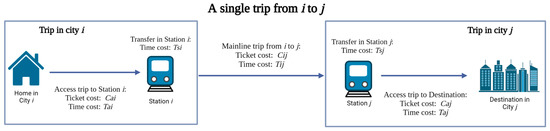 Figure 2. A single trip from city to city .
Living costs, including accommodation and food expenditure, were also considered to assess a real passenger’s decision-making process and behaviour. A ‘dual-city life’ traveller who was assumed to live and work in two different cities and , commutes by HSR every day, pays the living costs at the price level of city , and receives a salary from working in city .
- Rent cost in city ;
- Food cost in city ;
- Total living cost in city ;
Because the time cost has a different unit of measurement from the monetary cost, it needs to be converted into monetary cost, indicated as , according to the equivalent value of time. The method, value of time (VOT), will be introduced in the following chapter.
- Total cost: ;
- Travel time: ;
- Travel monetary cost: ;
- Living cost: ;
- Basic form of economic accessibility: .
2.2. Passengers’ Travelling Behaviour and Different Levels of the Accessibility Indicators
Daily and weekly commuting is the most usual frequency for people who work 5 days a week. The three levels of the indicators classify the commute intensity and corresponding travel benefit levels.
In a journey from to :
Level 1: HSR Daily commuting return accessibility (DACC): passenger travels to the destination and back in one day without a fixed work time budget.
- Travel time with return: ;
- Travel monetary cost: ;
- Living cost: ;
- Total cost: ;
- DACC: .
Level 2: HSR Daily 8 h work return accessibility (DWACC): passenger travels to the destination and back in one day on HSR with a fixed 8 h working schedule.
- Travel time with return: ;
- Travel monetary cost: ;
- Living cost: ;
- Total cost: ;
- DWACC:.
Level 3: HSR Weekly return accessibility (WACC): passenger commutes between work city and home city weekly with 5 days living in the work city and the weekend spent in the home city.
- Travel time with return: 5 workdays living at : ; daily intracity commute travel time in : ; 2 weekend intercity trip from to : ;
- Travel monetary cost: 5 workdays living at : ; daily intracity commute travel time in : ; 2 weekend intercity trip from to : ;
- Living cost: 5 workdays living at : ; 2 weekend intercity trip from to : ;
- Total cost: ;
- DWACC: .
The DACC indicator, reflecting the average profit level of dual-city life based on a daily return trip by HSR, has a flexible time restriction, which only limits the total travel time within 24 h, without any fixed working time requirement in . The tester needs to receive the income in , and pay the living cost in , and the travel cost between the two cities. The DWACC indicator has a more severely restricted time budget. One traveller has a fixed 8 h of working time at place and commutes on HSR between and within one day. The time budgets of level 1 and level 2 accessibility represent the efficiency under different transport network speed levels. In an ideal situation, the result should indicate that the fast traffic service can support daily intercity commuter travel over a longer distance, breaking the level 1 economic accessibility value from 0. If the speed is high enough, allowing for the extra working time budget, the level 2 value would also increase to above 0. Level 3 accessibility, WACC, has the most relaxed time budget, representing the benefit level of travelling on the normal-speed railway service. The traveller would spend 5 days in place and return to at the weekend, with 5 days income and living cost at the average level in , two days travel and living costs in , and weekly intercity travel cost. Sometimes, the slow inner-city traffic takes even more time than is spent on HSR. To evaluate the influence of the low-efficiency access time on the overall journey, the original plan considered multiple inner-city travel modes. Due to the difficulty of collecting historical data, the bus service was considered to be the only approach for inner-city travel between the station and destination in the case study.
Monetary Measurement of Travel Time and Willingness to Pay
Because the travel friction element contains time and monetary costs which are measured by incomparable units, the travel time cost data need to be converted into a monetary unit for calculation. This procedure is indicated as . There are many ways to convert travel time into a monetary value. Generalised cost has been widely used as a conversion solution in modern traffic analysis [44]. The travel time cost, subdivided into access time, waiting time, main travel time, and congestion time, etc., is converted into the equivalent monetary units according to the suggested VOT evaluated by a traffic research organisation or government transport department, but this has also been opposed by some scholars due to a conflict with traditional consumer demand theory [45]. A report from the Victoria Transport Policy Institute systematically introduced travel cost and benefit analysis cases around the main developed countries [46]. It summarises the equivalent monetary values used in the different countries. In 2003, the UK Department for Transport (DfT) evaluated an average cost of 6.6 pence per minute for daily commuting and 5.9 p/min for other trips, which does not include business trips [47]; in 2014, the US Department of Transport (USDOT) also assessed VOT based on different modes of travel [48]. For surface traffic such as road traffic and slow-speed services except for HSR, the VOT was around USD 12 per hour for personal travel and USD 22.90 for business in 2011. Due to the different case samples and travel modes, it is necessary to clarify the VOT conversion process. Travel time saving and willingness to pay (WTP) have been tested in many empirical case studies. Burris et al.’s research tested the WTP method with different types of road users of the Katy Freeway toll lanes in Texas, illustrating that over 10% of drivers would like to pay extra for faster lanes, at USD 40 per hour [49]; Brownstone and Small’s research also drew a similar value (USD 20 to 40) from commuter travel analysis [50]. In Europe, Björklund and Swärdh estimated the WTP for more comfortable travel with a lower passenger density at around £2 [51].
- : the value of time;
- and : the monetary cost of fast and slow service;
- and : the time cost of fast and slow service;
- : the change in the travel monetary cost for faster service;
- : the change in the travel time cost for faster service;
- : the travel time from point to ;
- : journey monetary time cost calculating process.
In modern traffic systems, various modes of travel support a gradient of the time and cost combination which provides travellers with different choices. The extra expenditure paid for faster travel speed, WTP, can be considered as the price that the passenger would like to pay for the saveable time. Every traveller could be regarded as one service-upgraded passenger who had paid the WTP cost for the journey time saved by the travel mode with higher speed. If ideal market and technology conditions can a supply ‘differentiable’ traffic service, the marginal cost for the higher-speed service is the value of the time. In this research, the case study scale is limited to high-speed and lower-speed railway services.
2.3. Accessibility Validation and Application of Economic Analysis
An econometric panel regression model was constructed to validate the applicability of the accessibility indicator and analyse the differences in economic factors influenced by differences in transport connection or living profit level, such as population migration, labour force supply, certain industry outputs, etc., in empirical analysis. Economic accessibility is a directional variable because DACC, DWACC, and WACC are calculated based on a service’s direction and the results for the two directions between two cities can be dramatically different due to the exchange of working and living places. Therefore, it optimised the usage of statistical data by generating two groups of accessibility values and doubled the data size with only one service and two cities’ statistical data.
In addition to the three accessibility indicators as the explaining variables, a control variable SACCD was introduced, to represent the difference in single-city living profit level. The reason for development disparity should not only contain the intercity travel accessibility but also needs to consider the local profit level difference. The regress result is expected to acquire the corresponding parameter , of each accessibility indicator. The parameter’s robustness check and value can explain what the high-speed and slow-speed services can bring, how much they can impact the target, and if the single-city lifestyle starts to shift to an intercity one.
- and : start point and destination;
- : research period, 1 to n;
- : explained variable; difference (population, industry output) between i and j;
- : accessibility value matrix;
- : daily accessibility; : daily working accessibility with a fixed 8 h working time budget; : weekly working accessibility; : difference in single-city accessibility between and (control variable);
- , , , : parameters of the different levels of the corresponding ACC index;
- : time-invariant variable; : composite error term.
3. Case Study
3.1. Research Samples and Materials
3.1.1. Sample Cities and Research Period
- East China high-speed railway network.
In the past two decades, HSR has developed rapidly in China. The first HSR that connected the cities of Hefei and Nanjing was opened in August 2008. Until 2010, the Shanghai–Beijing and Nanjing–Shanghai services transported hundreds of millions of passengers and linked China’s economic and political centres, establishing the basic framework of the China high-speed railway network (CHR). In the following years, the network was extended and covered most of the provincial capitals around the east of China. The period from 2005 to 2015, with a 3-year non-HSR service period and 8 years of HSR development, was selected for the case study, to reflect the popularising progress of HSR. Five main HSR hub cities, Hefei, Wuhan, Nanjing, Shanghai, and Hangzhou, were selected to be the core sample cities as the service departure points and destinations. Another six cities at the edge of the area, Beijing, Jinan, Changsha, Tianjin, Nanchang, and Fuzhou, were introduced as the service destinations. The case samples and service structure are shown in Figure 3 and Figure 4. The whole sample pool could generate a panel with data from 55 high-speed services and 11 years for accessibility estimation and model validation.
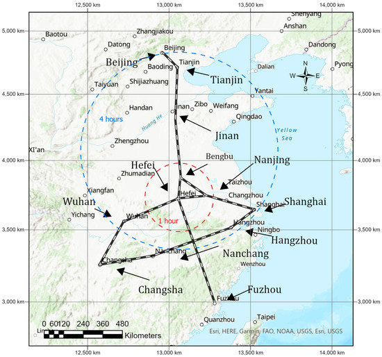
Figure 3.
East China high-speed network.
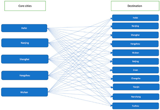
Figure 4.
High-speed railway service structure in the case study.
3.1.2. Materials, Data Collection, and Processing
Based on the methodology of the travel profit accessibility measurement, groups of economic and travel indicators that are listed in Table 2 are set for each case city in the accessibility measurement.
Table 2.
Accessibility measurement variables.
- The economic data were collected from each city’s official Statistical Yearbook published by the statistical bureau of each year.
- The intracity access information was collected from www.amap.com, a professional GIS.
- High-speed and normal-speed mainline railway service timetables and data were collected from www.12306.cn, the official railway information platform published by the China State Railway Group Company, Ltd., Beijing, China.
3.1.3. Consumer Price Index (CPI)
The case research period is from 2005 to 2015. Due to inflation and economic development, the price level kept changing. To eliminate price discrepancies, the year 2005 was regarded as the base period, and all price data were converted according to the local price level, including the intercity travel cost and inner-city access travel monetary cost. The data processing example is shown in Table 3.
Table 3.
Hefei economic data process.
3.1.4. Collection of Inner-City Travel Information
The sample cities mainly are the capitals of each province, with a large urban area and many sub-districts. The modern HSR stations are usually located far away from the city centre. Travellers may have activity in any place in the city, generating different inner-city travel times and cost data. To reflect the real access time and monetary cost from any location in the sample city to its HSR station, the start point and destination are assumed to be the geographical centre of every sub-district. The related access time and monetary cost are equal to the average time and ticket cost value from the station to these local centres. Although most cities developed rapidly and expanded in scale from 2005 to 2015, the access time is still assumed to be the same as in 2015, to reduce the stress of searching the very detailed historical data. Furthermore, the monetary cost was also assumed to be the current public transport cost because there was only an average increase of less than CNY 5 in these sample cities over 10 years according to the limited historic city traffic material, which accounts for a very small part of the whole journey cost.
3.1.5. Intercity Travel
Due to the difficulty of collecting historical travel data, the normal-speed railway service was considered to be the mode of intercity travel in the non-HSR years. Although road transport also occupied a large part of the market, it is too complicated to collect historical data and information. Estimation of the value of travel time relied on how much the traveller would like to pay for faster transport modes, the so-called WTP methodology. So, the normal-speed train, which is slower than HSR, was assumed to be the exclusive mode of travel for estimating intercity passengers’ time and cost.
3.2. Accessibility Measurement
To demonstrate the accessibility calculation process, the case of the Hefei–Nanjing HSR is introduced as an example. Hefei is the departure city for living, and Nanjing is the destination for working. The intercity traveller needs to pay the necessary living cost at the Hefei price level, including food and accommodation, and the travel cost to Nanjing. In terms of benefits, the assumed traveller works in Nanjing and is paid at Nanjing’s average salary. All the monetary costs are converted to the price level in 2005 by the deflator for Hefei each year, as shown in Table 4. In the case of reversed service direction from Nanjing to Hefei, the traveller needs to pay the fares for living in Nanjing, which were converted by the deflator for Nanjing as well. The coloured font in the bottom rows indicates the data which were influenced by modification of statistical standards after 2014.
Table 4.
Hefei–Nanjing intercity living cost.
The travel time cost and monetary cost are shown in Table 5. The access time, HSR travel time, and normal-speed rail travel time were collected from the integrated data. The station time, including waiting time, transit time, and others, was assumed to be 10 min. The ‘daily work time restriction’ and ‘reachable time restriction’ are the work time budget for assessing if the high-speed commuter service or normal-speed commuter service could support 8 h of work time or just let the travellers have a return trip in one day. A value ‘one′ means the time budget is satisfied and ‘zero′ means it is not. In the following part, the monetary cost is listed with the same structure of travel progress and corresponding monetary cost, and it was also converted by the living city’s deflator. The year 2008 is the first year with high-speed service; the change in travel cost can be recognised clearly.
Table 5.
Hefei–Nanjing travel friction.
The passenger’s travel time value is estimated according to their WTP. The calculation process was shown in Table 6. In the case of Hefei to Nanjing, the normal-speed train, taking 1.76 h, was considered to be the only way to travel without HSR, and the mainline time monetary cost per hour was CNY 23,580 in 2005. In 2008, the new HSR service increased it to CNY 28,472, but the total journey time cost dropped to CNY 160, which indicates that HSR has higher unit VOT costs, but the large volume of the saved time could bring more benefits. The steady ticket price and CPI help to lower the travel cost further.
Table 6.
Hefei–Nanjing value of travel time.
Table 7 shows the final statistical results for accessibility. In theory, the benefit part of the DWACC should be higher than the part of the DACC, to reflect the extra profit brought by the steady working time. In the case study, it is simplified by using the same attractiveness part for the estimation, and the only difference is the 8 h work time requirement. If the time budget cannot be satisfied, the ‘real daily work accessibility’ would be zero, which means the opportunity is unachievable. In addition, the ‘weekly accessibility’ needs to consider the 5 days’ living cost in the work city and 2 days’ living cost in the home city, which illustrates the traveller’s weekly return lifestyle. The full accessibility calculation is listed in the next section.
Table 7.
Hefei–Nanjing three levels of accessibility.
3.3. All Level 1, Level 2, and Level 3 Accessibility Calculation Results
The three omitted tables, Table 8, Table 9 and Table 10, show the value for three levels of accessibility for the journey departing from Hefei or Nanjing to the other cities. The corresponding full table can be found in Table A1, Table A2 and Table A3 in the Appendix A.
Table 8.
The example of Daily return accessibility.
Table 9.
The example of Daily return accessibility with 8 h work schedule.
Table 10.
The example of Weekly return accessibility.
In the results, the blue font indicates the HSR opening years and red font highlights the data affected by modification of the statistical standards. The accessibility values of the services connecting to other core cities were higher than the services linked to peripheral cities. The values for the three levels of accessibility, DACC, DWACC, and WACC, are all far less than one. This means that cross-city travel is very expensive as a high-frequency mode of daily commuter travel for most people. By comparing the time series data for each city, the most significant improvement is that the HSR made the daily intercity commute possible and broke the zero profit ratio. The new service expanded the travel distance and made more opportunities achievable.
However, according to the DWACC value with a regulated time budget, the current HSR cannot satisfy the requirement with a fixed 8 h of work time. However, the index could indicate that the new high-speed service successfully expanded the area for the traveller who has intercity living and working requirements. In Figure 5, the DWACC values of Hefei are selected and integrated with the high-speed railway construction progress into a group of heat maps. In the figure, the colour from light blue to deep yellow indicates DWACC strength, matching the value from 0 to 1. For the city of Hefei, yellow colour represents the level of intracity living accessibility ratio, which is the highest level generating positive net profit. The first panel shows the level in 2005 without the high-speed service. The remaining five panels illustrate the DWACC strength change following HSR construction. The intercity living profit ability dramatically improved, and the area covered by the heatmap expanded and became deeper at more places, due to the faster traffic conditions and economic development.

Figure 5.
Hefei DWACC strength change and HSR railway construction progress indicated by heat map: (a) The DWACC Level and HSR service network from Hefei to the other sample cities in 2005; (b) The DWACC strength and HSR service network from Hefei to the other sample cities in 2008; (c) The DWACC strength and HSR service network from Hefei to the other sample cities in 2009; (d) The DWACC strength and HSR service network from Hefei to the other sample cities in 2010; (e) The DWACC strength and HSR service network from Hefei to the other sample cities in 2012; (f) The DWACC strength and HSR service network from Hefei to the other sample cities in 2015.
The level of weekly return commute, WACC, shows a better result with an average value 0.2 higher than the results for ‘daily return’ and ‘8 h work return’. Travellers spending 5 days in the work city and going back home on the weekend is a better choice. The relatively loose time budget of weekly return commuters would also need to face the competition between the normal-speed train and HSR. Following a reduction in travel frequency, for example, to monthly, the profit would increase and be close to the level for single-city life in the work city; though this is meaningless. On the other hand, the HSR ticket price and inner-city travel costs kept steady in the research period. The HSR ticket price increased by 30% to 50% compared to that for the normal-speed train. This makes the travel profit ratio fall for the service over a short distance, and the new service was not able to reduce travel time enough in the early years when the new HSR had just opened. However, due to rapid economic growth, faster train speed, and larger HSR line capacity, the ACC value quickly regained a new level, especially on the service between Hefei and Nanjing.
The accessibility index was calculated based on the collected average income and travel cost data, which indicated the profit level of a common commuter. Through the distribution of national income, the size of the population that could achieve a higher profit level from intercity travel can be evaluated. By adjusting the OPP value and the travel friction, the accessibility index can classify the variable travel profit into several tiers with different commuter incomes and investigate the urbanisation process. Figure 6 shows the urbanisation process and corresponding accessibility index in three stages. If the national income followed an ideal normal distribution, the faster service speed and suitable journey cost would push the better profit area to the left, eliminating the gap between single-city life and cross-city life. Combining the indicators of the average-income traveller’s accessibility value and local national income distribution could reflect the progress of the urban integration process.
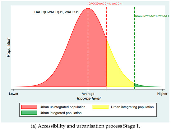
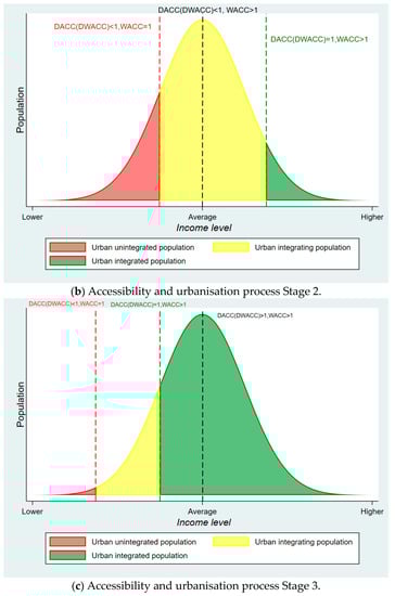
Figure 6.
Three stages of the urbanisation process indicated by Accessibility change.
3.4. Validation of Accessibility Indicators
The three indicators were also validated through econometric model analysis, to investigate if the designed index can explain the practical economic change. The registered population difference (RPD) between the departure city and the destination city was set to be the explained variable in the validation model. Hefei, Nanjing, and Shanghai represent three levels of city in the transportation network, from developing to developed. Four fixed-effect regression panels, the All-cities panel and three sub-panels, the Hefei, Nanjing, and Shanghai departure panels, contain the three levels of accessibility indicators and the single-city accessibility difference (SACCD) from 2005 to 2015. The result was shown in Table 11.
Table 11.
Panel test results summary.
- All-cities panel: data from 50 services, departing from 5 core cities to each other and the other 6 peripheral cities, containing the variables: RPD, DACC, DWACC, WACC, and SACCD, over 11 years, with a total of 550 observations;
- Hefei, Nanjing, and Shanghai panels: data from 10 services, departing to the other 10 cities, containing RPD, DACC, DWACC, WACC, and SACCD, over 11 years, with a total of 110 observations.
- DACC and WACC.
The population difference regression fitted well on the All-cities, Hefei, and Nanjing panels. The p-value indicated the high significance of DACC and WACC, at 99%. In the Shanghai panel, DACC is not as significant as in the other cases, but DWACC (p < 0.06) and WACC (p < 0.12) could affect the explained variables effectively. DACC measures the benefit level of an HSR user and WACC represents that of a normal-speed railway user. By comparing both variables’ parameters, it can be found that DACC has a negative impact on RPD, but WACC shows a positive impact, which means the HSR could help to eliminate the population gap between the departure city and destination city, but the normal-speed service could enlarge it.
Observing the parameters, DACC showed 3 to 4 times greater strength than WACC, which indicates that the high-speed service has a heavier weight in reducing the population gap and it is also strong enough to counteract the opposite effect brought by the slow-speed service in the research period. Shanghai, as the megacity in the east network, has the largest population, which far exceeds that of the other case cities with a positive population difference value. The DACC parameter is insignificant in the Shanghai panel regression, which means that the high-speed service started from Shanghai to the other cities did not have a dramatic effect on decreasing the population gap.
- DWACC.
DWACC, with an additional 8 h working time budget, reflects an extremely frequent commute travel scenario. The p-value for DWACC in the regression for the All-cities, Hefei, and Nanjing panels is insignificant. However, in the case of Shanghai, the p-value is less than 0.06 and the parameter reached +1.635, which indicates that DWACC can significantly affect the population gap between Shanghai and the other destination. Following the increasing DWACC value, the population gap would be enlarged. Due to Shanghai’s population advantage, if more services can satisfy the 8 h working time budget, more people may expect to move to Shanghai and take HSR to the other city for work. Compared to the other cities with a smaller economy, travellers from the top-level cities have different intercity travel preferences.
- SACCD.
SACCD as a control variable measured the difference in single-city living benefit level between the departure city and destination city, representing fluctuations affected by the attraction of the city itself rather than the travel service. In the analysis, SACCD has a significant impact on the population difference with the positive parameter passing the robustness check (p < 0.05) in the All-cities and Hefei panels and returning a p-value < 0.15 in the other cases, which corresponds to the motivation for population migration in reality. Living conditions and income level can be regarded as important factors affecting the population difference whereas, compared to DACC, DWACC, and WACC, SACCD did not have the same strength, which was only approximately one-sixth that of DACC. The major power of population migration is more related to traffic conditions.
4. Conclusions
In this paper, a methodology for measuring economic accessibility was proposed. Three levels of accessibility indicators were designed according to the traveller’s commuting frequency and time arrangement, establishing a connection between railway services’ technical and economic data. It supports a new perspective, from the view of the average traveller’s benefit level, to discuss a transport system’s utility and its economic impact. The commute trip, with stricter requirements of the transport system, is considered by most people for planning their living strategy. The economic efficiency and timeliness of the travel mode can affect the traveller’s income level and living arrangements. The economic accessibility measurement simulates this process from the view of a normal commuter, thinking of the traveller’s benefit and cost analysis. By understanding the economic influencing principle and mechanism through proper accessibility indicators, transport system designers and policymakers can evaluate traffic flow and local economic development before starting a new travel service. HSR development has reshaped people’s travel behaviour, urban layouts, and economic structure, promoting urbanisation progress, and it is an ideal study object to test economic accessibility indicators.
Eleven cities in the east CHR network, five core hub cities in the centre and six cities at the edge, were selected as the samples for empirical analysis. Data from over 50 services, containing both high-speed and slow-speed railway service history data, inner-city traffic data, city economy data, and demographic data, were collected to evaluate accessibility. The results for the three levels of accessibility illustrate that intercity life with a daily cross-city HSR commute is still not a good choice for most people at the current stage with a travel distance of 400 km or over. However, considering the possible national income distribution, intercity life for people at the top level should be profitable. The most dramatic contribution is that the new HSR service realised the availability of daily intercity commuter trips between more and more cities. In particular, on the services linking the cities located at the edge of the slow-speed railway network with a travel time of over 7 h, a one-day return journey, even with 8 h of work time scheduled, has become achievable, generating and delivering more opportunities. Transport and living costs significantly affect the performance and efficiency of the overall travel system. Intercity travel expenditure is higher than the normal intracity living cost. Following economic development and inflation, a steady public transport price level could reduce the cost of social productivity and generate more profitable travel for people with a lower income, emphasising the public character of the HSR service; although, different countries have various facility ownership, operation, and management structures with different pricing processes. The panel regression model, which applied three levels of accessibility indicators and investigated how travel service speed and cost affect population migration between cities, proved that the modern high-speed service could help to disperse the population, reducing the difference between a developed city and a developing one. On the other hand, the traditional slow-speed service could reverse this progress, enlarging the population difference and aggregating the labour force, leading to a local core city. On the other hand, by comparing the parameters, the HSR has approximately 6 to 7 times greater strength than the conventional railway service and it has become the main travel-related power of local population migration.
Author Contributions
Conceptualization, E.Z.; methodology, E.Z.; software, E.Z.; validation, E.Z.; investigation, E.Z.; resources, E.Z.; data curation, E.Z.; writing—original draft preparation, E.Z.; writing—review and editing, L.C., P.K. and D.G.D.; visualization, E.Z.; supervision, L.C., P.K. and D.G.D.; project administration, L.C. All authors have read and agreed to the published version of the manuscript.
Funding
This research received no external funding.
Institutional Review Board Statement
Not applicable.
Informed Consent Statement
Not applicable.
Data Availability Statement
The data that support the findings of this study are available from the corresponding author upon reasonable request.
Conflicts of Interest
The authors declare no conflict of interest.
List of Abbreviation/Glossary of Terms
| Term | Explanation/Meaning/Definition |
| ACC | Accessibility |
| CHR | China high-speed railway network |
| CNY | Chinese Yuan |
| CPI | Consumer price index |
| DACC | Daily Commute Accessibility |
| DWACC | Daily Work Commute Accessibility |
| GIS | Geographic information system |
| HSR | High-speed railway |
| OPP | Travel benefits and opportunities |
| PPA | Potential path area |
| PPS | Potential path space |
| RPD | Registered population difference |
| SACCD | Single-city accessibility difference |
| SSR | Slow-speed railway service |
| TGV | French high-speed railway |
| VOT | Value of travel time |
| WACC | Weekly Commute Accessibility |
| WTP | Willingness to pay |
Appendix A
Table A1.
Daily return accessibility.
Table A1.
Daily return accessibility.
| DACC | Hefei | ||||||||||
|---|---|---|---|---|---|---|---|---|---|---|---|
| Year | Hefei | Nanjing | Shanghai | Wuhan | Hangzhou | Beijing | Jinan | Changsha | Tianjin | Nanchang | Fuzhou |
| 2005 | - | 0.152 | 0.148 | 0.133 | 0.182 | 0.000 | 0.052 | 0.000 | 0.000 | 0.084 | 0.000 |
| 2006 | - | 0.176 | 0.163 | 0.150 | 0.207 | 0.000 | 0.058 | 0.000 | 0.000 | 0.091 | 0.000 |
| 2007 | - | 0.206 | 0.190 | 0.175 | 0.240 | 0.000 | 0.069 | 0.000 | 0.000 | 0.106 | 0.000 |
| 2008 | - | 0.190 | 0.215 | 0.217 | 0.268 | 0.000 | 0.080 | 0.000 | 0.000 | 0.123 | 0.000 |
| 2009 | - | 0.206 | 0.230 | 0.139 | 0.298 | 0.000 | 0.087 | 0.000 | 0.000 | 0.132 | 0.000 |
| 2010 | - | 0.225 | 0.134 | 0.156 | 0.329 | 0.000 | 0.097 | 0.075 | 0.000 | 0.146 | 0.000 |
| 2011 | - | 0.255 | 0.153 | 0.178 | 0.144 | 0.000 | 0.111 | 0.086 | 0.000 | 0.166 | 0.000 |
| 2012 | - | 0.284 | 0.168 | 0.200 | 0.157 | 0.068 | 0.116 | 0.099 | 0.059 | 0.185 | 0.000 |
| 2013 | - | 0.309 | 0.183 | 0.219 | 0.164 | 0.075 | 0.127 | 0.107 | 0.057 | 0.204 | 0.000 |
| 2014 | - | 0.326 | 0.197 | 0.244 | 0.000 | 0.082 | 0.137 | 0.116 | 0.062 | 0.225 | 0.000 |
| 2015 | - | 0.349 | 0.204 | 0.266 | 0.000 | 0.098 | 0.140 | 0.126 | 0.067 | 0.043 | 0.000 |
| Nanjing | |||||||||||
| Year | Hefei | Nanjing | Shanghai | Wuhan | Hangzhou | Beijing | Jinan | Changsha | Tianjin | Nanchang | Fuzhou |
| 2005 | 0.097 | - | 0.137 | 0.000 | 0.092 | 0.000 | 0.084 | 0.000 | 0.000 | 0.000 | 0.000 |
| 2006 | 0.111 | - | 0.156 | 0.000 | 0.106 | 0.000 | 0.095 | 0.000 | 0.000 | 0.000 | 0.000 |
| 2007 | 0.132 | - | 0.178 | 0.000 | 0.121 | 0.000 | 0.111 | 0.000 | 0.000 | 0.000 | 0.000 |
| 2008 | 0.124 | - | 0.091 | 0.000 | 0.136 | 0.000 | 0.128 | 0.000 | 0.000 | 0.000 | 0.000 |
| 2009 | 0.137 | - | 0.103 | 0.121 | 0.153 | 0.000 | 0.139 | 0.000 | 0.000 | 0.000 | 0.000 |
| 2010 | 0.154 | - | 0.115 | 0.141 | 0.171 | 0.000 | 0.157 | 0.053 | 0.000 | 0.000 | 0.000 |
| 2011 | 0.180 | - | 0.131 | 0.161 | 0.282 | 0.069 | 0.087 | 0.061 | 0.066 | 0.000 | 0.061 |
| 2012 | 0.203 | - | 0.144 | 0.186 | 0.308 | 0.076 | 0.098 | 0.071 | 0.065 | 0.000 | 0.069 |
| 2013 | 0.223 | - | 0.151 | 0.210 | 0.320 | 0.084 | 0.107 | 0.076 | 0.064 | 0.000 | 0.076 |
| 2014 | 0.234 | - | 0.233 | 0.236 | 0.000 | 0.092 | 0.117 | 0.084 | 0.070 | 0.055 | 0.077 |
| 2015 | 0.255 | - | 0.248 | 0.260 | 0.000 | 0.111 | 0.120 | 0.091 | 0.075 | 0.061 | 0.083 |
| Shanghai | |||||||||||
| Year | Hefei | Nanjing | Shanghai | Wuhan | Hangzhou | Beijing | Jinan | Changsha | Tianjin | Nanchang | Fuzhou |
| 2005 | 0.076 | 0.122 | - | 0.000 | 0.231 | 0.000 | 0.000 | 0.000 | 0.000 | 0.000 | 0.000 |
| 2006 | 0.086 | 0.141 | - | 0.000 | 0.266 | 0.000 | 0.000 | 0.000 | 0.000 | 0.000 | 0.000 |
| 2007 | 0.102 | 0.162 | - | 0.000 | 0.162 | 0.000 | 0.000 | 0.026 | 0.000 | 0.042 | 0.000 |
| 2008 | 0.117 | 0.084 | - | 0.000 | 0.189 | 0.000 | 0.000 | 0.029 | 0.000 | 0.047 | 0.000 |
| 2009 | 0.128 | 0.092 | - | 0.062 | 0.209 | 0.000 | 0.000 | 0.033 | 0.000 | 0.054 | 0.050 |
| 2010 | 0.076 | 0.101 | - | 0.070 | 0.240 | 0.000 | 0.000 | 0.037 | 0.000 | 0.060 | 0.056 |
| 2011 | 0.089 | 0.114 | - | 0.080 | 0.284 | 0.034 | 0.062 | 0.042 | 0.045 | 0.069 | 0.064 |
| 2012 | 0.102 | 0.129 | - | 0.091 | 0.321 | 0.039 | 0.070 | 0.049 | 0.052 | 0.080 | 0.074 |
| 2013 | 0.111 | 0.140 | - | 0.099 | 0.341 | 0.042 | 0.076 | 0.053 | 0.056 | 0.086 | 0.080 |
| 2014 | 0.117 | 0.149 | - | 0.111 | 0.000 | 0.045 | 0.082 | 0.058 | 0.061 | 0.094 | 0.087 |
| 2015 | 0.126 | 0.159 | - | 0.121 | 0.000 | 0.049 | 0.084 | 0.063 | 0.066 | 0.102 | 0.095 |
| Wuhan | |||||||||||
| Year | Hefei | Nanjing | Shanghai | Wuhan | Hangzhou | Beijing | Jinan | Changsha | Tianjin | Nanchang | Fuzhou |
| 2005 | 0.081 | 0.000 | 0.000 | - | 0.000 | 0.000 | 0.000 | 0.085 | 0.000 | 0.101 | 0.000 |
| 2006 | 0.092 | 0.000 | 0.000 | - | 0.000 | 0.000 | 0.000 | 0.097 | 0.000 | 0.109 | 0.000 |
| 2007 | 0.110 | 0.000 | 0.000 | - | 0.000 | 0.000 | 0.000 | 0.116 | 0.000 | 0.126 | 0.000 |
| 2008 | 0.126 | 0.000 | 0.000 | - | 0.000 | 0.000 | 0.000 | 0.133 | 0.000 | 0.144 | 0.000 |
| 2009 | 0.117 | 0.127 | 0.100 | - | 0.000 | 0.000 | 0.030 | 0.061 | 0.000 | 0.156 | 0.000 |
| 2010 | 0.130 | 0.139 | 0.110 | - | 0.000 | 0.000 | 0.033 | 0.068 | 0.000 | 0.094 | 0.000 |
| 2011 | 0.151 | 0.157 | 0.124 | - | 0.101 | 0.000 | 0.038 | 0.095 | 0.000 | 0.106 | 0.000 |
| 2012 | 0.171 | 0.177 | 0.137 | - | 0.111 | 0.037 | 0.043 | 0.110 | 0.000 | 0.121 | 0.000 |
| 2013 | 0.188 | 0.193 | 0.150 | - | 0.116 | 0.041 | 0.046 | 0.118 | 0.000 | 0.133 | 0.086 |
| 2014 | 0.192 | 0.201 | 0.160 | - | 0.000 | 0.042 | 0.050 | 0.127 | 0.000 | 0.145 | 0.086 |
| 2015 | 0.207 | 0.216 | 0.165 | - | 0.000 | 0.046 | 0.051 | 0.138 | 0.000 | 0.158 | 0.092 |
| Hangzhou | |||||||||||
| Year | Hefei | Nanjing | Shanghai | Wuhan | Hangzhou | Beijing | Jinan | Changsha | Tianjin | Nanchang | Fuzhou |
| 2005 | 0.104 | 0.083 | 0.261 | 0.000 | - | 0.000 | 0.306 | 0.000 | 0.000 | 0.065 | 0.000 |
| 2006 | 0.118 | 0.096 | 0.288 | 0.000 | - | 0.000 | 0.352 | 0.000 | 0.000 | 0.071 | 0.000 |
| 2007 | 0.140 | 0.110 | 0.170 | 0.000 | - | 0.000 | 0.410 | 0.030 | 0.000 | 0.042 | 0.000 |
| 2008 | 0.157 | 0.123 | 0.189 | 0.000 | - | 0.000 | 0.190 | 0.034 | 0.000 | 0.048 | 0.000 |
| 2009 | 0.171 | 0.133 | 0.201 | 0.000 | - | 0.000 | 0.206 | 0.038 | 0.000 | 0.051 | 0.061 |
| 2010 | 0.190 | 0.147 | 0.223 | 0.000 | - | 0.000 | 0.225 | 0.043 | 0.000 | 0.057 | 0.069 |
| 2011 | 0.087 | 0.239 | 0.252 | 0.067 | - | 0.039 | 0.255 | 0.049 | 0.049 | 0.065 | 0.079 |
| 2012 | 0.099 | 0.269 | 0.278 | 0.076 | - | 0.044 | 0.284 | 0.057 | 0.049 | 0.073 | 0.089 |
| 2013 | 0.108 | 0.293 | 0.303 | 0.084 | - | 0.048 | 0.309 | 0.061 | 0.047 | 0.081 | 0.098 |
| 2014 | 0.120 | 0.340 | 0.354 | 0.097 | - | 0.051 | 0.326 | 0.068 | 0.052 | 0.091 | 0.102 |
| 2015 | 0.131 | 0.367 | 0.368 | 0.107 | - | 0.056 | 0.349 | 0.074 | 0.057 | 0.100 | 0.110 |
The blue font indicates the HSR opening years and red font highlights the data affected by modification of the statistical standards.
Table A2.
Daily return accessibility with 8 h work schedule.
Table A2.
Daily return accessibility with 8 h work schedule.
| DWACC | Hefei | ||||||||||
|---|---|---|---|---|---|---|---|---|---|---|---|
| Year | Hefei | Nanjing | Shanghai | Wuhan | Hangzhou | Beijing | Jinan | Changsha | Tianjin | Nanchang | Fuzhou |
| 2005 | - | 0.152 | 0.000 | 0.000 | 0.000 | 0.000 | 0.000 | 0.000 | 0.000 | 0.000 | 0.000 |
| 2006 | - | 0.176 | 0.000 | 0.000 | 0.000 | 0.000 | 0.000 | 0.000 | 0.000 | 0.000 | 0.000 |
| 2007 | - | 0.206 | 0.000 | 0.000 | 0.000 | 0.000 | 0.000 | 0.000 | 0.000 | 0.000 | 0.000 |
| 2008 | - | 0.190 | 0.000 | 0.000 | 0.000 | 0.000 | 0.000 | 0.000 | 0.000 | 0.000 | 0.000 |
| 2009 | - | 0.206 | 0.000 | 0.139 | 0.000 | 0.000 | 0.000 | 0.000 | 0.000 | 0.000 | 0.000 |
| 2010 | - | 0.225 | 0.134 | 0.156 | 0.000 | 0.000 | 0.000 | 0.075 | 0.000 | 0.000 | 0.000 |
| 2011 | - | 0.255 | 0.153 | 0.178 | 0.144 | 0.000 | 0.000 | 0.086 | 0.000 | 0.000 | 0.000 |
| 2012 | - | 0.284 | 0.168 | 0.200 | 0.157 | 0.068 | 0.116 | 0.099 | 0.059 | 0.000 | 0.000 |
| 2013 | - | 0.309 | 0.183 | 0.219 | 0.164 | 0.075 | 0.127 | 0.107 | 0.057 | 0.000 | 0.000 |
| 2014 | - | 0.326 | 0.197 | 0.244 | 0.000 | 0.082 | 0.137 | 0.116 | 0.062 | 0.000 | 0.000 |
| 2015 | - | 0.349 | 0.204 | 0.266 | 0.000 | 0.098 | 0.140 | 0.126 | 0.067 | 0.043 | 0.000 |
| Nanjing | |||||||||||
| Year | Hefei | Nanjing | Shanghai | Wuhan | Hangzhou | Beijing | Jinan | Changsha | Tianjin | Nanchang | Fuzhou |
| 2005 | 0.097 | - | 0.137 | 0.000 | 0.000 | 0.000 | 0.000 | 0.000 | 0.000 | 0.000 | 0.000 |
| 2006 | 0.111 | - | 0.156 | 0.000 | 0.000 | 0.000 | 0.000 | 0.000 | 0.000 | 0.000 | 0.000 |
| 2007 | 0.132 | - | 0.178 | 0.000 | 0.000 | 0.000 | 0.000 | 0.000 | 0.000 | 0.000 | 0.000 |
| 2008 | 0.124 | - | 0.091 | 0.000 | 0.000 | 0.000 | 0.000 | 0.000 | 0.000 | 0.000 | 0.000 |
| 2009 | 0.137 | - | 0.103 | 0.121 | 0.000 | 0.000 | 0.000 | 0.000 | 0.000 | 0.000 | 0.000 |
| 2010 | 0.154 | - | 0.115 | 0.141 | 0.000 | 0.000 | 0.000 | 0.053 | 0.000 | 0.000 | 0.000 |
| 2011 | 0.180 | - | 0.131 | 0.161 | 0.282 | 0.069 | 0.087 | 0.061 | 0.066 | 0.000 | 0.000 |
| 2012 | 0.203 | - | 0.144 | 0.186 | 0.308 | 0.076 | 0.098 | 0.071 | 0.065 | 0.000 | 0.000 |
| 2013 | 0.223 | - | 0.151 | 0.210 | 0.320 | 0.084 | 0.107 | 0.076 | 0.064 | 0.000 | 0.000 |
| 2014 | 0.234 | - | 0.233 | 0.236 | 0.000 | 0.092 | 0.117 | 0.084 | 0.070 | 0.055 | 0.000 |
| 2015 | 0.255 | - | 0.248 | 0.260 | 0.000 | 0.111 | 0.120 | 0.091 | 0.075 | 0.061 | 0.000 |
| Shanghai | |||||||||||
| Year | Hefei | Nanjing | Shanghai | Wuhan | Hangzhou | Beijing | Jinan | Changsha | Tianjin | Nanchang | Fuzhou |
| 2005 | 0.000 | 0.122 | - | 0.000 | 0.231 | 0.000 | 0.000 | 0.000 | 0.000 | 0.000 | 0.000 |
| 2006 | 0.000 | 0.141 | - | 0.000 | 0.266 | 0.000 | 0.000 | 0.000 | 0.000 | 0.000 | 0.000 |
| 2007 | 0.000 | 0.162 | - | 0.000 | 0.162 | 0.000 | 0.000 | 0.026 | 0.000 | 0.042 | 0.000 |
| 2008 | 0.000 | 0.084 | - | 0.000 | 0.189 | 0.000 | 0.000 | 0.029 | 0.000 | 0.047 | 0.000 |
| 2009 | 0.000 | 0.092 | - | 0.062 | 0.209 | 0.000 | 0.000 | 0.033 | 0.000 | 0.054 | 0.050 |
| 2010 | 0.076 | 0.101 | - | 0.070 | 0.240 | 0.000 | 0.000 | 0.037 | 0.000 | 0.060 | 0.056 |
| 2011 | 0.089 | 0.114 | - | 0.080 | 0.284 | 0.034 | 0.062 | 0.042 | 0.045 | 0.069 | 0.064 |
| 2012 | 0.102 | 0.129 | - | 0.091 | 0.321 | 0.039 | 0.070 | 0.049 | 0.052 | 0.080 | 0.074 |
| 2013 | 0.111 | 0.140 | - | 0.099 | 0.341 | 0.042 | 0.076 | 0.053 | 0.056 | 0.086 | 0.080 |
| 2014 | 0.117 | 0.149 | - | 0.111 | 0.000 | 0.045 | 0.082 | 0.058 | 0.061 | 0.094 | 0.087 |
| 2015 | 0.126 | 0.159 | - | 0.121 | 0.000 | 0.049 | 0.084 | 0.063 | 0.066 | 0.102 | 0.095 |
| Wuhan | |||||||||||
| Year | Hefei | Nanjing | Shanghai | Wuhan | Hangzhou | Beijing | Jinan | Changsha | Tianjin | Nanchang | Fuzhou |
| 2005 | 0.000 | 0.000 | 0.000 | - | 0.000 | 0.000 | 0.000 | 0.085 | 0.000 | 0.101 | 0.000 |
| 2006 | 0.000 | 0.000 | 0.000 | - | 0.000 | 0.000 | 0.000 | 0.097 | 0.000 | 0.109 | 0.000 |
| 2007 | 0.000 | 0.000 | 0.000 | - | 0.000 | 0.000 | 0.000 | 0.116 | 0.000 | 0.126 | 0.000 |
| 2008 | 0.000 | 0.000 | 0.000 | - | 0.000 | 0.000 | 0.000 | 0.133 | 0.000 | 0.144 | 0.000 |
| 2009 | 0.117 | 0.127 | 0.100 | - | 0.000 | 0.000 | 0.000 | 0.061 | 0.000 | 0.156 | 0.000 |
| 2010 | 0.130 | 0.139 | 0.110 | - | 0.000 | 0.000 | 0.000 | 0.068 | 0.000 | 0.094 | 0.000 |
| 2011 | 0.151 | 0.157 | 0.124 | - | 0.101 | 0.000 | 0.000 | 0.095 | 0.000 | 0.106 | 0.000 |
| 2012 | 0.171 | 0.177 | 0.137 | - | 0.111 | 0.037 | 0.000 | 0.110 | 0.000 | 0.121 | 0.000 |
| 2013 | 0.188 | 0.193 | 0.150 | - | 0.116 | 0.041 | 0.000 | 0.118 | 0.000 | 0.133 | 0.000 |
| 2014 | 0.192 | 0.201 | 0.160 | - | 0.000 | 0.042 | 0.000 | 0.127 | 0.000 | 0.145 | 0.000 |
| 2015 | 0.207 | 0.216 | 0.165 | - | 0.000 | 0.046 | 0.000 | 0.138 | 0.000 | 0.158 | 0.000 |
| Hangzhou | |||||||||||
| Year | Hefei | Nanjing | Shanghai | Wuhan | Hangzhou | Beijing | Jinan | Changsha | Tianjin | Nanchang | Fuzhou |
| 2005 | 0.000 | 0.000 | 0.261 | 0.000 | - | 0.000 | 0.000 | 0.000 | 0.000 | 0.000 | 0.000 |
| 2006 | 0.000 | 0.000 | 0.288 | 0.000 | - | 0.000 | 0.000 | 0.000 | 0.000 | 0.000 | 0.000 |
| 2007 | 0.000 | 0.000 | 0.170 | 0.000 | - | 0.000 | 0.000 | 0.030 | 0.000 | 0.042 | 0.000 |
| 2008 | 0.000 | 0.000 | 0.189 | 0.000 | - | 0.000 | 0.000 | 0.034 | 0.000 | 0.048 | 0.000 |
| 2009 | 0.000 | 0.000 | 0.201 | 0.000 | - | 0.000 | 0.000 | 0.038 | 0.000 | 0.051 | 0.061 |
| 2010 | 0.000 | 0.000 | 0.223 | 0.000 | - | 0.000 | 0.000 | 0.043 | 0.000 | 0.057 | 0.069 |
| 2011 | 0.087 | 0.239 | 0.252 | 0.067 | - | 0.039 | 0.062 | 0.049 | 0.049 | 0.065 | 0.079 |
| 2012 | 0.099 | 0.269 | 0.278 | 0.076 | - | 0.044 | 0.070 | 0.057 | 0.049 | 0.073 | 0.089 |
| 2013 | 0.108 | 0.293 | 0.303 | 0.084 | - | 0.048 | 0.077 | 0.061 | 0.047 | 0.081 | 0.098 |
| 2014 | 0.120 | 0.340 | 0.354 | 0.097 | - | 0.051 | 0.085 | 0.068 | 0.052 | 0.091 | 0.102 |
| 2015 | 0.131 | 0.367 | 0.368 | 0.107 | - | 0.056 | 0.087 | 0.074 | 0.057 | 0.100 | 0.110 |
The blue font indicates the HSR opening years and red font highlights the data affected by modification of the statistical standards.
Table A3.
Weekly return accessibility.
Table A3.
Weekly return accessibility.
| WACC | Hefei | ||||||||||
|---|---|---|---|---|---|---|---|---|---|---|---|
| Year | Hefei | Nanjing | Shanghai | Wuhan | Hangzhou | Beijing | Jinan | Changsha | Tianjin | Nanchang | Fuzhou |
| 2005 | - | 0.411 | 0.498 | 0.419 | 0.556 | 0.297 | 0.188 | 0.235 | 0.232 | 0.305 | 0.233 |
| 2006 | - | 0.465 | 0.539 | 0.460 | 0.610 | 0.332 | 0.210 | 0.258 | 0.259 | 0.326 | 0.258 |
| 2007 | - | 0.537 | 0.596 | 0.520 | 0.691 | 0.370 | 0.246 | 0.290 | 0.294 | 0.366 | 0.297 |
| 2008 | - | 0.489 | 0.649 | 0.609 | 0.740 | 0.414 | 0.282 | 0.324 | 0.375 | 0.415 | 0.339 |
| 2009 | - | 0.524 | 0.684 | 0.453 | 0.792 | 0.442 | 0.301 | 0.358 | 0.410 | 0.441 | 0.357 |
| 2010 | - | 0.567 | 0.445 | 0.497 | 0.840 | 0.472 | 0.335 | 0.279 | 0.456 | 0.468 | 0.391 |
| 2011 | - | 0.624 | 0.500 | 0.547 | 0.452 | 0.523 | 0.377 | 0.319 | 0.498 | 0.520 | 0.443 |
| 2012 | - | 0.680 | 0.541 | 0.590 | 0.496 | 0.254 | 0.390 | 0.362 | 0.214 | 0.573 | 0.486 |
| 2013 | - | 0.725 | 0.578 | 0.635 | 0.511 | 0.277 | 0.415 | 0.377 | 0.204 | 0.616 | 0.517 |
| 2014 | - | 0.763 | 0.613 | 0.663 | 0.000 | 0.300 | 0.445 | 0.398 | 0.219 | 0.649 | 0.491 |
| 2015 | - | 0.810 | 0.612 | 0.702 | 0.000 | 0.361 | 0.437 | 0.427 | 0.235 | 0.154 | 0.519 |
| Nanjing | |||||||||||
| Year | Hefei | Nanjing | Shanghai | Wuhan | Hangzhou | Beijing | Jinan | Changsha | Tianjin | Nanchang | Fuzhou |
| 2005 | 0.277 | - | 0.399 | 0.223 | 0.327 | 0.282 | 0.290 | 0.201 | 0.230 | 0.287 | 0.219 |
| 2006 | 0.311 | - | 0.449 | 0.271 | 0.367 | 0.317 | 0.323 | 0.223 | 0.258 | 0.308 | 0.245 |
| 2007 | 0.366 | - | 0.492 | 0.326 | 0.414 | 0.349 | 0.369 | 0.248 | 0.289 | 0.343 | 0.278 |
| 2008 | 0.336 | - | 0.266 | 0.396 | 0.452 | 0.389 | 0.419 | 0.277 | 0.367 | 0.387 | 0.317 |
| 2009 | 0.366 | - | 0.299 | 0.428 | 0.496 | 0.421 | 0.449 | 0.310 | 0.406 | 0.417 | 0.337 |
| 2010 | 0.406 | - | 0.329 | 0.484 | 0.540 | 0.453 | 0.501 | 0.213 | 0.455 | 0.445 | 0.372 |
| 2011 | 0.462 | - | 0.370 | 0.532 | 0.794 | 0.261 | 0.282 | 0.244 | 0.247 | 0.494 | 0.242 |
| 2012 | 0.502 | - | 0.402 | 0.587 | 0.876 | 0.285 | 0.314 | 0.278 | 0.241 | 0.549 | 0.270 |
| 2013 | 0.537 | - | 0.415 | 0.647 | 0.889 | 0.310 | 0.336 | 0.293 | 0.230 | 0.594 | 0.292 |
| 2014 | 0.561 | - | 0.632 | 0.681 | 0.000 | 0.339 | 0.364 | 0.314 | 0.248 | 0.206 | 0.287 |
| 2015 | 0.596 | - | 0.654 | 0.725 | 0.000 | 0.409 | 0.362 | 0.340 | 0.267 | 0.225 | 0.307 |
| Shanghai | |||||||||||
| Year | Hefei | Nanjing | Shanghai | Wuhan | Hangzhou | Beijing | Jinan | Changsha | Tianjin | Nanchang | Fuzhou |
| 2005 | 0.282 | 0.376 | - | 0.118 | 0.567 | 0.134 | 0.239 | 0.200 | 0.189 | 0.269 | 0.250 |
| 2006 | 0.316 | 0.428 | - | 0.133 | 0.631 | 0.152 | 0.266 | 0.221 | 0.210 | 0.300 | 0.277 |
| 2007 | 0.368 | 0.485 | - | 0.152 | 0.418 | 0.178 | 0.304 | 0.101 | 0.234 | 0.167 | 0.303 |
| 2008 | 0.408 | 0.257 | - | 0.174 | 0.476 | 0.202 | 0.344 | 0.114 | 0.257 | 0.187 | 0.332 |
| 2009 | 0.440 | 0.279 | - | 0.253 | 0.514 | 0.220 | 0.368 | 0.128 | 0.290 | 0.212 | 0.195 |
| 2010 | 0.279 | 0.304 | - | 0.281 | 0.575 | 0.241 | 0.409 | 0.143 | 0.318 | 0.233 | 0.216 |
| 2011 | 0.320 | 0.338 | - | 0.312 | 0.664 | 0.133 | 0.221 | 0.163 | 0.177 | 0.266 | 0.247 |
| 2012 | 0.354 | 0.377 | - | 0.347 | 0.756 | 0.151 | 0.248 | 0.188 | 0.203 | 0.305 | 0.281 |
| 2013 | 0.379 | 0.405 | - | 0.377 | 0.791 | 0.164 | 0.265 | 0.199 | 0.214 | 0.325 | 0.299 |
| 2014 | 0.395 | 0.430 | - | 0.406 | 0.000 | 0.171 | 0.288 | 0.214 | 0.232 | 0.347 | 0.315 |
| 2015 | 0.416 | 0.456 | - | 0.430 | 0.000 | 0.186 | 0.286 | 0.231 | 0.250 | 0.371 | 0.337 |
| Wuhan | |||||||||||
| Year | Hefei | Nanjing | Shanghai | Wuhan | Hangzhou | Beijing | Jinan | Changsha | Tianjin | Nanchang | Fuzhou |
| 2005 | 0.295 | 0.305 | 0.200 | - | 0.291 | 0.148 | 0.224 | 0.266 | 0.197 | 0.343 | 0.242 |
| 2006 | 0.330 | 0.349 | 0.219 | - | 0.327 | 0.167 | 0.251 | 0.297 | 0.221 | 0.368 | 0.270 |
| 2007 | 0.387 | 0.399 | 0.247 | - | 0.369 | 0.198 | 0.288 | 0.343 | 0.248 | 0.404 | 0.306 |
| 2008 | 0.432 | 0.440 | 0.275 | - | 0.403 | 0.225 | 0.328 | 0.389 | 0.316 | 0.455 | 0.347 |
| 2009 | 0.400 | 0.462 | 0.381 | - | 0.442 | 0.244 | 0.109 | 0.184 | 0.348 | 0.487 | 0.367 |
| 2010 | 0.440 | 0.500 | 0.412 | - | 0.477 | 0.266 | 0.122 | 0.202 | 0.389 | 0.302 | 0.401 |
| 2011 | 0.497 | 0.549 | 0.460 | - | 0.364 | 0.306 | 0.138 | 0.278 | 0.423 | 0.337 | 0.451 |
| 2012 | 0.538 | 0.604 | 0.502 | - | 0.403 | 0.140 | 0.155 | 0.318 | 0.410 | 0.377 | 0.498 |
| 2013 | 0.573 | 0.647 | 0.537 | - | 0.417 | 0.153 | 0.167 | 0.333 | 0.383 | 0.411 | 0.317 |
| 2014 | 0.581 | 0.671 | 0.564 | - | 0.000 | 0.158 | 0.179 | 0.349 | 0.403 | 0.433 | 0.305 |
| 2015 | 0.612 | 0.711 | 0.564 | - | 0.000 | 0.172 | 0.180 | 0.374 | 0.427 | 0.464 | 0.324 |
| Hangzhou | |||||||||||
| Year | Hefei | Nanjing | Shanghai | Wuhan | Hangzhou | Beijing | Jinan | Changsha | Tianjin | Nanchang | Fuzhou |
| 2005 | 0.362 | 0.316 | 0.641 | 0.199 | - | 0.130 | 0.239 | 0.220 | 0.183 | 0.252 | 0.285 |
| 2006 | 0.403 | 0.363 | 0.690 | 0.222 | - | 0.147 | 0.266 | 0.243 | 0.205 | 0.270 | 0.316 |
| 2007 | 0.467 | 0.413 | 0.435 | 0.252 | - | 0.173 | 0.304 | 0.116 | 0.230 | 0.160 | 0.355 |
| 2008 | 0.506 | 0.451 | 0.472 | 0.285 | - | 0.195 | 0.342 | 0.129 | 0.289 | 0.181 | 0.397 |
| 2009 | 0.537 | 0.481 | 0.498 | 0.308 | - | 0.210 | 0.362 | 0.144 | 0.316 | 0.195 | 0.230 |
| 2010 | 0.588 | 0.526 | 0.539 | 0.344 | - | 0.232 | 0.405 | 0.160 | 0.356 | 0.213 | 0.255 |
| 2011 | 0.301 | 0.800 | 0.599 | 0.255 | - | 0.154 | 0.224 | 0.183 | 0.199 | 0.238 | 0.289 |
| 2012 | 0.333 | 0.858 | 0.652 | 0.285 | - | 0.174 | 0.251 | 0.210 | 0.195 | 0.268 | 0.323 |
| 2013 | 0.358 | 0.905 | 0.694 | 0.311 | - | 0.190 | 0.269 | 0.223 | 0.186 | 0.293 | 0.347 |
| 2014 | 0.402 | 1.066 | 0.792 | 0.353 | - | 0.204 | 0.301 | 0.246 | 0.206 | 0.322 | 0.353 |
| 2015 | 0.432 | 1.116 | 0.788 | 0.382 | - | 0.223 | 0.301 | 0.266 | 0.222 | 0.349 | 0.377 |
The blue font indicates the HSR opening years and red font highlights the data affected by modification of the statistical standards.
References
- Vickerman, R. High-speed rail in Europe: Experience and issues for future development. Ann. Reg. Sci. 1997, 31, 21–38. [Google Scholar] [CrossRef]
- Masson, S.; Petiot, R. Can the high speed rail reinforce tourism attractiveness? The case of the high speed rail between Perpignan (France) and Barcelona (Spain). Technovation 2009, 29, 611–617. [Google Scholar] [CrossRef]
- De Rus, G.; Inglada, V. Cost-benefit analysis of the high-speed train in Spain. Ann. Reg. Sci. 1997, 31, 175–188. [Google Scholar] [CrossRef]
- De Rus, G.; Nombela, G. Is Investment in High Speed Rail Socially Profitable? J. Transp. Econ. Policy 2007, 41, 3–23. [Google Scholar]
- Fröidh, O. Market effects of regional high-speed trains on the Svealand line. J. Transp. Geogr. 2005, 13, 352–361. [Google Scholar] [CrossRef]
- Gutiérrez, J.; González, R.; Gómez, G. The European high-speed train network: Predicted effects on accessibility patterns. J. Transp. Geogr. 1996, 4, 227–238. [Google Scholar] [CrossRef]
- Behrens, C.; Pels, E. Intermodal competition in the London–Paris passenger market: High-Speed Rail and air transport. J. Urban Econ. 2012, 71, 278–288. [Google Scholar] [CrossRef]
- Hsu, C.-I.; Chung, W.-M. A model for market share distribution between high-speed and conventional rail services in a transportation corridor. Ann. Reg. Sci. 1997, 31, 121–153. [Google Scholar] [CrossRef]
- Kim, K.S. High-speed rail developments and spatial restructuring: A case study of the Capital region in South Korea1. Cities 2000, 17, 251–262. [Google Scholar] [CrossRef]
- Givoni, M. Development and Impact of the Modern High-speed Train: A Review. Transp. Rev. 2006, 26, 593–611. [Google Scholar] [CrossRef]
- Okada, H. Features and economic and social effects of the Shinkansen. Jpn. Railw. Transp. Rev. 1994, 3, 9–16. [Google Scholar]
- Sasaki, K.; Ohashi, T.; Ando, A. High-speed rail transit impact on regional systems: Does the Shinkansen contribute to dispersion? Ann. Reg. Sci. 1997, 31, 77–98. [Google Scholar] [CrossRef]
- Wang, X.; Huang, S.; Zou, T.; Yan, H. Effects of the high speed rail network on China’s regional tourism development. Tour. Manag. Perspect. 2012, 1, 34–38. [Google Scholar] [CrossRef]
- Xiaoyan, L.; Xiaojun, C.; Yunfeng, B.; Xingmei, H. Influence on Beijing-Tianjin intercity high-speed railway to regional economic by quantitative analysis. Railw. Econ. Res. 2010, 5, 5–11. [Google Scholar]
- Wang, F.; Wei, X.; Liu, J.; He, L.; Gao, M. Impact of high-speed rail on population mobility and urbanisation: A case study on Yangtze River Delta urban agglomeration, China. Transp. Res. Part A Policy Pract. 2019, 127, 99–114. [Google Scholar] [CrossRef]
- Ingram, D.R. The concept of accessibility: A search for an operational form. Reg. Stud. 1971, 5, 101–107. [Google Scholar] [CrossRef]
- Baxter, R.; Lenzi, G. The measurement of relative accessibility. Reg. Stud. 1975, 9, 15–26. [Google Scholar] [CrossRef]
- Guy, C.M. The Assessment of Access to Local Shopping Opportunities: A Comparison of Accessibility Measures. Environ. Plan. B Plan. Des. 1983, 10, 219–237. [Google Scholar] [CrossRef]
- Stanilov, K. Accessibility and Land Use: The Case of Suburban Seattle, 1960–1990. Reg. Stud. 2003, 37, 783–794. [Google Scholar] [CrossRef]
- Willigers, J.; Van Wee, B. High-speed rail and office location choices. A stated choice experiment for the Netherlands. J. Transp. Geogr. 2011, 19, 745–754. [Google Scholar] [CrossRef]
- Taaffe, E.J.; Gauthier, H.L.; O’Kelly, M.E. Geography of Transportation, 2nd ed.; Prentice Hall: Upper Saddle River, NJ, USA, 1996. [Google Scholar]
- Ben-Akiva, M.E.; Lerman, S.R. Disaggregate Travel and Mobility-Choice Models and Measures of Accessibility. In Behavioural Travel Modelling; Routledge: Abingdon-on-Thames, UK, 2021; pp. 654–679. [Google Scholar]
- Baradaran, S.; Ramjerdi, F. Performance of accessibility measures in Europe. J. Transp. Stat. 2001, 4, 31–48. [Google Scholar]
- Niemeier, D.A. Accessibility: An evaluation using consumer welfare. Transportation 1997, 24, 377–396. [Google Scholar] [CrossRef]
- Levine, J. Rethinking accessibility and jobs-housing balance. J. Am. Plan. Assoc. 1998, 64, 133–149. [Google Scholar] [CrossRef]
- Wachs, M.; Kumagai, T.G. Physical accessibility as a social indicator. Socio Econ. Plan. Sci. 1973, 7, 437–456. [Google Scholar] [CrossRef]
- Cracknell, B. Accessibility to the countryside as a factor in planning for leisure. Reg. Stud. 1967, 1, 147–161. [Google Scholar] [CrossRef]
- Sherman, L.; Barber, B.; Kondo, W. Method for evaluating metropolitan accessibility. Transp. Res. Rec. 1974, 499, 70–82. [Google Scholar]
- Cascetta, E.; Cartenì, A.; Montanino, M. A behavioral model of accessibility based on the number of available opportunities. J. Transp. Geogr. 2016, 51, 45–58. [Google Scholar] [CrossRef]
- Miller, H.J. Measuring space-time accessibility benefits within transportation networks: Basic theory and computational procedures. Geogr. Anal. 1999, 31, 187–212. [Google Scholar] [CrossRef]
- Miller, H.J.; Wu, Y.-H. GIS software for measuring space-time accessibility in transportation planning and analysis. GeoInformatica 2000, 4, 141–159. [Google Scholar] [CrossRef]
- Berglund, S. Path-based accessibility. J. Transp. Stat. 2001, 4, 79–91. [Google Scholar]
- Hansen, W.G. How accessibility shapes land use. J. Am. Inst. Plan. 1959, 25, 73–76. [Google Scholar] [CrossRef]
- Dalvi, M.Q.; Martin, K. The measurement of accessibility: Some preliminary results. Transportation 1976, 5, 17–42. [Google Scholar] [CrossRef]
- Harris, C.D. The, Market as a Factor in the Localization of Industry in the United States. Ann. Assoc. Am. Geogr. 1954, 44, 315–348. [Google Scholar] [CrossRef]
- Linneker, B.J.; Spence, N.A. Accessibility measures compared in an analysis of the impact of the M25 London Orbital Motorway on Britain. Environ. Plan. A 1992, 24, 1137–1154. [Google Scholar] [CrossRef]
- Gutiérrez, J. Location, economic potential and daily accessibility: An analysis of the accessibility impact of the high-speed line Madrid–Barcelona–French border. J. Transp. Geogr. 2001, 9, 229–242. [Google Scholar] [CrossRef]
- Haynes, K.E. Labor markets and regional transportation improvements: The case of high-speed trains an introduction and review. Ann. Reg. Sci. 1997, 31, 57–76. [Google Scholar] [CrossRef]
- Cascetta, E.; Cartenì, A.; Henke, I.; Pagliara, F. Economic growth, transport accessibility and regional equity impacts of high-speed railways in Italy: Ten years ex post evaluation and future perspectives. Transp. Res. Part A Policy Pract. 2020, 139, 412–428. [Google Scholar] [CrossRef]
- Xiaohua, S.; Debin, Y.; Ran, L. Study on Radiated Regions of Railway Node Cities along Beijing-Shanghai High-speed Railway Based on Gravity Model. Logist. Technol. 2015, 34, 136–139. [Google Scholar]
- Deyou, M.; Yuqi, L. Strength and Direction of Regional Economic Linkage in Jiangsu Province Based on Gravity Model. Prog. Geogr. 2009, 28, 697–704. [Google Scholar]
- Yang, Q.; Wang, Y.; Liu, Y.; Liu, J.; Hu, X.; Ma, J.; Wang, X.; Wan, Y.; Hu, J.; Zhang, Z.; et al. The impact of China’s high-speed rail investment on regional economy and air pollution emissions. J. Environ. Sci. 2023, 131, 26–36. [Google Scholar] [CrossRef]
- Chen, Z. Measuring the regional economic impacts of high-speed rail using a dynamic SCGE model: The case of China. Eur. Plan. Stud. 2019, 27, 483–512. [Google Scholar] [CrossRef]
- Lesley, L. Generalised costs and the value of time as a method of patronage forecasting. Acta Tech. Jaurinensis 2009, 2, 57–68. [Google Scholar]
- Goodwin, P. Generalised time and the problem of equity in transport studies. Transportation 1974, 3, 1–23. [Google Scholar] [CrossRef]
- Litman, T. Transportation cost and benefit analysis. Vic. Transp. Policy Inst. 2020, 31, 1–19. [Google Scholar]
- Mackie, P.; Wardman, M.; Fowkes, A.S.; Whelan, G.; Nellthorp, J.; Bates, J. Values of Travel Time Savings UK; Working Paper; Institute of Transport Studies, University of Leeds: Leeds, UK, 2003. [Google Scholar]
- Ayala, R.; Rogoff, P. Revised Departmental Guidance on Valuation of Travel Time in Economic Analysis; Office of Transportation Policy: Washington, DC, USA, 2014.
- Burris, M.; Spiegelman, C.; Abir, A.; Lee, S. Travelers’ Value of Time and Reliability as Measured on Katy Freeway; No. PRC 15-37 F; Texas A&M Transportation Institute: Bryan, TX, USA, 2016. [Google Scholar]
- Brownstone, D.; Small, K.A. Valuing time and reliability: Assessing the evidence from road pricing demonstrations. Transp. Res. Part A Policy Pract. 2005, 39, 279–293. [Google Scholar] [CrossRef]
- Björklund, G.; Swärdh, J.-E. Valuing in-Vehicle Comfort and Crowding Reduction in Public Transport; No. 2015: 12; CTS-Centre for Transport Studies Stockholm (KTH and VTI): Stockholm, Sweden, 2015. [Google Scholar]


Disclaimer/Publisher’s Note: The statements, opinions and data contained in all publications are solely those of the individual author(s) and contributor(s) and not of MDPI and/or the editor(s). MDPI and/or the editor(s) disclaim responsibility for any injury to people or property resulting from any ideas, methods, instructions or products referred to in the content. |
© 2023 by the authors. Licensee MDPI, Basel, Switzerland. This article is an open access article distributed under the terms and conditions of the Creative Commons Attribution (CC BY) license (https://creativecommons.org/licenses/by/4.0/).