A Robust Model Predictive Control for a Photovoltaic Pumping System Subject to Actuator Saturation Nonlinearity

Abstract

In this paper, a new robust model predictive control (RMPC) for uncertain nonlinear systems subject to actuator saturation is designed to regulate the terminal voltage of a photovoltaic generator (PVG) that feeds a DC motor-pump via a buck DC–DC converter. The considered system is a combination of a PVG-converter and DC motor-pump, which possesses nonlinear behavior along with under a saturating control signal highly dependent on the operation point and climate conditions of solar radiation and temperature. As a result, the control task is complex due to the nonlinearity of the system and its dependence on climate conditions. Based on the dead-zone property, the presented paper introduces a new RMPC technique to provide an innovative and efficient solution to ensure the closed-loop system’s robust stability in the presence of actuator nonlinearity. In this paper, the nonlinear system is described in polytypic form, and an appropriate linear feedback control law is designed and used to minimize an infinite horizon cost function under the framework of linear matrix inequalities (LMIs). Furthermore, sufficient state-feedback control law conditions are synthesized to guarantee the robust stability of the closed-loop system in the presence of polytypic uncertainties. Simulation results are provided, in which the results illustrate the effectiveness of the proposed method.

1. Introduction

Over the past three decades, solar energy has become increasingly popular as one of the main renewable energy sources. Several strategies have been introduced to use sunlight as a source of energy in which sunlight can be converted into heat (solar–thermal energy conversion) [1], electricity (solar–photovoltaic energy conversion) [2], solar fuel (hydrogen) generated via photocatalytic water splitting [3,4], or sunlight chemicals, such as ${\mathrm{H}}_2{\mathrm{O}}_2$ production [5]. It can also be used for ${\mathrm{CO}}_2$reduction [6] and ammonia synthesis [7]. The use of photovoltaic energy has grown tremendously in a wide range of applications, where many non-electrified villages and rural regions rely on solar energy as their primary source of electricity since electrification is difficult and expensive [8,9]. In addition, photovoltaic water-pumping systems for irrigation and water supply in remote areas have been widely implemented due to their unique features of ease of installation, environment friendliness, and low maintenance costs [10,11]. For the optimization of energy, PV water-pumping systems have to operate at their maximum power point (MPP). A directly coupled PV electromechanical system operates at the intersection of current–voltage curves of the PV array and DC motor-pump set [12,13]. PV water-pumping systems are usually designed to extract as much energy as possible from the solar resource, using a simple DC–DC power converter controlled by an maximum power point tracker (MPPT) algorithm [14,15]. In the literature, many of the MPPT algorithms have been applied for obtaining the maximal power from PV systems. Perturb and observe (P&O) and incremental conductance (INC) are the most widely used methods [16,17,18]. However, the simplest and fastest algorithm is the constant voltage control approach, in which the PV array is controlled to operate at a constant voltage equal to the MPP voltage of the array at the standard test condition (STC) provided by the manufacturer, by adjusting the duty ratio of the power converter [15]. The authors in [19,20] have shown that this technique has improved stability and low dependence on solar irradiation. Elgendy et al. [13] proved in a comparative investigation that it offers significantly better energy use efficiencies (up to about 91%) compared to directly connected systems without taking the effects of insolation and temperature variations on the MPP voltage into consideration.

Generally, the dynamic behavior of power converter systems can be described as a bilinear model under a saturating control signal. The classical control techniques applied to power converters usually do not take into account input saturation, which can severely degrade the performance of the closed-loop system, thus making the closed-loop system unstable, especially if the converter is subject to large perturbation. Furthermore, when a power converter is used in solar applications, the control system becomes more complex. Many studies have lately demonstrated that PVG characteristics have a substantial effect on the dynamic behavior of power converters [21]. Since the PVG dynamic resistance is both an environmental variable and operating point dependent, major changes in the PV system might compromise its stability [15].

Despite the nonlinearity and uncertainty of these systems, the linear (state or output) feedback control of power converters based on the small signal control theory proposed by Middlebrook and Cuk [22] is the most applicable approach at present. For example, the fuzzy-logic controller proposed in [23] and the PID controller proposed in [24] are based on small signal control theory. Such linear controllers are designed based on the model linearization at a certain operation point, and the obtained model can only be useful for small variations around that specific steady point [25,26]. To cope with the deficiency of these linear controllers, several nonlinear control strategies have been developed with stability analysis, including fuzzy-logic controllers [27,28], adaptive control [29,30], neural-network-based control [31], sliding mode control (SMC) [32], and feedback linearization controllers [33]. However, these methods have two major limitations: The constraints on the input actuators are not considered when using these methods. In addition, the closed-loop performance in terms of robust stability and the presence of parameter uncertainties is not optimized. In recent years, more consideration has been given to studying intelligent and robust control structures, which can maintain nonlinear systems stability over a certain operating range.

Model predictive control (MPC) is a control strategy that offers attractive solutions for controlling constrained linear or nonlinear systems [34,35]. The ability to handle hard constraints on states/outputs and inputs and time-varying behaviors make the MPC method an effective technique for a wide range of practical applications [36]. MPC algorithms are widely based on dynamic models to predict system behaviors over a prediction horizon. The reliable solution obtained is based on the minimization at each time step of an upper bound of the worst-case infinite horizon quadratic function.

In general, it is difficult to construct an accurate model of a system in which uncertainty is frequently present. It is well known that the uncertainty related to systems can be represented in the form of parametric uncertainty or bounded disturbance regions. In the presence of a significant level of uncertainty, the control law designed by MPC based on a nominal model is suboptimal and can even be infeasible. Unfortunately, traditional MPC approaches fail to explicitly handle the plant-model uncertainty. As a result, numerous researchers have recently shown great interest in the RMPC of uncertain systems, where several tools, such as the LMI optimization approach, were developed to build RMPC algorithms [37,38,39,40].

In most practical control processes, actuator saturation is a common kind of nonlinearity. The classical control techniques that ignore actuator saturation may severely reduce the performance of a closed-loop system, and the closed-loop system may lose its stability, especially if subjected to certain large perturbations [41,42]. Hence, it is important to consider the control input constraints in the RMPC design. In the literature, stability analysis and the synthesis of RMPC strategies for linear systems with actuator saturation have been considered as a popular topic in the past few decades. The common feature of most RMPC strategies is that they deal with input nonlinearity by estimating the domain of attraction in the presence of actuator saturation. Kothare et al. [37] proposed a new robust centralized constrained MPC technique using an LMI-based optimization approach to guarantee the asymptotic stability of closed-loop systems. The proposed algorithm allows the incorporation of a large class of plant uncertainty descriptions and can guarantee the stability and robustness of the controlled system. The design in [37] also includes systematic treatment of input and state constraints. Casavola et al. [38] presented a scheduling min-max MPC algorithm for linear parameter varying (LPV) systems with polytopic uncertainty subject to input saturation. Cao and Lin [43] proposed an RMPC algorithm for LPV systems with polytopic uncertainty in the presence of actuator saturation. In the approach in [43], the actuator saturation constraint was characterized in terms of the convex hull of a group of auxiliary linear feedback laws and an actual linear feedback law. Huanga et al. [44] improved the design in [43] by taking the relative weighting between the auxiliary and actual feedback laws into account. Despite the improvements obtained, this method does not consider certain issues of system nonlinearity. Another disadvantage is that the real-time implementation of this approach suffers from a heavy computational burden due to the large number of inequalities when the saturating linear feedback law is expressed on a convex hull. This may lead to the intractability of the optimization problem, especially in the case of high-dimensional systems and fast sampling applications. Moreover, numerous MPC designs for linear systems with actuator saturation have been published in [45,46,47,48,49].

During the past decade, many MPC techniques for systems subject to actuator saturation have been studied. In [50], a model predictive tracking control algorithm for the flexible air-breathing hypersonic flight vehicle was proposed to handle the flight control problem with actuator constraints and input delays. A novel, fast MPC technique with actuator saturation for large-scale structures based on the explicit expression form of the Newmark-β method and parametric variational principle was introduced in [51]. In [52], the asymptotic stability of the finite horizon MPC of nonlinear systems with incremental input constraints was proposed and investigated. The authors in [53] presented an MPC approach for systems with a dead zone and saturation, where two different control strategies based on MPC were compared: the former uses hybrid MPC, while the latter is based on dead-zone inversion and standard MPC. A novel discrete-time sliding mode predictive control technique for a tethered satellite with saturated input was proposed and investigated in [54], in which a discrete-time auxiliary controller was involved in the discrete-time MPC scheme to achieve fast and more stable performance. However, in contrast to linear systems subject to actuator saturation, there are few significant MPC designs for nonlinear systems subject to actuator saturation.

In this work, the ability of the LMI approach is exploited to accommodate an MPC-based technique for the control of nonlinear systems subject to actuator saturation, through the dead-zone property. As the main contribution in this work, a new RMPC for uncertain nonlinear systems subject to actuator saturation is proposed to control a photovoltaic pumping system where a simulation study on the PV pumping system, which comprises a PVG, a voltage-mode-controlled DC–DC buck converter, and a DC motor-pump, is illustrated to evaluate the performance of the proposed controller. The objective of the control process is to keep the PVG voltage at the MPP voltage in the presence of PVG dynamic resistance uncertainty and atmospheric condition changes. The proposed RMPC algorithm innovatively uses certain ideas from the work in [55]. In the proposed approach, a saturation model based on dead-zone nonlinearity is used to handle the saturation of the control input. The controller design is characterized as an optimization problem of the worst-case performance objective function over an infinite moving horizon. In addition, at each time step, adequate state feedback that renders the closed-loop saturated nonlinear system globally asymptotically stable to the origin is obtained via linear matrix inequalities. The main advantages of the proposed approach, compared with other well-known RMPC techniques, are its ability to consider both actuator saturation and system nonlinearity and the reduction in conservativeness by avoiding a large number of inequalities when the actuator saturation constraint is characterized in terms of the convex hull; therefore, the proposed algorithm guarantees a lower computation time compared to other methods. The proposed method can be applied to deal with complex industrial systems, such as computer numerical control (CNC) machines, active magnetic bearing (AMB), robot manipulators, overhead cranes, and DC–DC power converters. Different scenarios are used in the simulation study to illustrate the effectiveness and applicability of the proposed approach to the PV pumping system.

The rest of this paper is organized as follows: Section 2 describes the mathematical formulation of the problem to be handled. Some basic concepts concerning MPC are introduced and the saturated RMPC scheme is proposed in Section 3 and Section 4, respectively. Next, several simulation results are demonstrated under the Matlab environment in Section 5 to test the validity and effectiveness of our method. Finally, the paper is concluded in Section 6.

2. Problem Formulation

Consider a nonlinear discrete-time dynamical system subject to actuator saturation:

$$x\left(k+1\right)=f\left(x\left(k\right),\overline{u}\left(k\right)\right)$$

(1)

where$k$ is the current time instant and $x\in {ℝ}^n$ is the state. The control input is bounded as $\overline{u}\left(k\right)=sat\left(u\left(k\right)\right)$. $sat\left(u\left(k\right)\right)\in {ℝ}^m$ is a saturation function of the control input $u\left(k\right)\in {ℝ}^m$, which is defined as:

$$sat\left(u\left(k\right)\right)=\{\begin{array}{ccc}-u_{lim},& if& u\left(k\right)<-u_{lim}\\ u\left(k\right),& if& -u_{lim}\le u\left(k\right)\le u_{lim}\\ u_{lim}& if& u\left(k\right)>u_{lim}\end{array}$$

(2)

where $u_{lim}$ is a control input limit and$u_{lim}=u_{max}$. $u_{max}$ is the maximum control input limit. $f\in {ℂ}^2$ is a nonlinear function of states and control inputs $f\left(0,0\right)=0$. Let $A={\frac{\partial f}{\partial x}|}_{\left(0,0\right)}$, $B={\frac{\partial f}{\partial u}|}_{\left(0,0\right)}$, and the dynamic system (Equation (1)) can be reformulated as a polytopic uncertain system:

$$x\left(k+1\right)=A\left(\beta \right)x\left(k\right)+B\left(\beta \right)\overline{u}\left(k\right)+\widetilde{ f}\left(x\left(k\right),\overline{u}\left(k\right)\right)$$

(3)

where the system matrices are affine functions of a parameter vector $\beta$ of $r$ parameters ($\beta =\left({\beta }_1,\dots ,{\beta }_r\right)$). Each uncertain parameter ${\beta }_j$ is bounded between a minimum and a maximum value $\overline{{\beta }_j}$and $\underset{\_}{{\beta }_j}$. $j=\left\{1,2,\dots ,r\right\}$

$${\beta }_j\in \left[\underset{\_}{{\beta }_j},\overline{{\beta }_j}\right]$$

(4)

Moreover, we assume that:

$$\left[A\left(\beta \right) B\left(\beta \right)\right]\in \Omega =Co\left\{\left[A_1 B_1\right],\left[A_2 B_2\right],\dots ,\left[A_r B_r\right]\right\}$$

(5)

where$\Omega$ denotes the convex hull and $\left[A_j B_j\right]$are vertices of the convex hull. $\Omega$ can be written as:

$$\left[A\left(\beta \right) B\left(\beta \right)\right]=\left\{{{\displaystyle \sum }}_{j=1}^r{\beta }_j\left[A_j B_j\right], {\beta }_j>0, {{\displaystyle \sum }}_{j=1}^r{\beta }_j=1\right\}$$

(6)

$\tilde{f}\left(x\left(k\right),\overline{u}\left(k\right)\right)$ is the nonlinear term obtained by differing between the nominal nonlinear model and the linear part, which is given by:

$$\widetilde{ f}\left(x\left(k\right),\overline{u}\left(k\right)\right)=f\left(x\left(k\right),\overline{u}\left(k\right)\right)-A_{j}x\left(k\right)+B_j\overline{u}\left(k\right)$$

(7)

Assume that $\tilde{f}$ is globally Lipschitz or at least locally Lipschitz in a region$\mathfrak{D}$ including the origin with respect to$x\left(k\right)$ and uniformly in $\overline{u}\left(k\right)$. Therefore, we have the following Lipschitz condition:

$$\left|\right|\tilde{f}\left(x,\overline{u}\right)-\tilde{f}{\left(x_0,\overline{u}\right)\left|\right|}_2 \le N\left|\right|x-x_0{\left|\right|}_2$$

(8)

$$\{\begin{array}{c}\forall x,x_0\in {ℝ}^n\mathrm{globally}\mathrm{Lipschitz}\\ \forall x,x_0\in \mathfrak{D}\mathrm{locally}\mathrm{Lipschitz}\end{array}$$

where $N\in {ℝ}^{n\times n}$ is a Lipschitz constant matrix. For $x_0=0$, the Lipschitz inequality (Equation (8)) can be rewritten as:

$${\left[\tilde{f}\left(x,\overline{u}\right)-\tilde{f}\left(0,\overline{u}\right)\right]}^{T}I\left[\tilde{f}\left(x,\overline{u}\right)-\tilde{f}\left(0,\overline{u}\right)\right]\le x^T{N}^{T}Nx$$

(9)

where $I$ is the identity matrix.

This paper aims to find a non-saturating linear-state feedback law $u\left(k\right)=Hx\left(k\right),$where a dead-zone nonlinearity approach is used to handle the saturation nonlinearity. Hence, the dynamic system (Equation (3)) is written as:

$$\begin{array}{ll}x\left(k+1\right)& =A_{j}x\left(k\right)+B_j\left(\overline{u}\left(k\right)-u\left(k\right)+u\left(k\right)\right)+\tilde{f}(x\left(k\right),\overline{u}\left(k\right))\\ & =\left(A_j+B_{j}H\right)x\left(k\right)+B_j\psi \left(k\right)+\tilde{f}(x\left(k\right),\overline{u}\left(k\right))\end{array}$$

(10)

where $H$is the state feedback gain. Let us introduce the following useful lemmas for later use.

Lemma 1.

For the saturation constraint defined by Equation (2), let:

$$\phi =\overline{u}-u$$

(11)

Thus, there is:

$${\phi }^T\phi \le ϵu^{T}u$$

(12)

where $0<ϵ<1$ and $\mathsf{\psi }={\left[{\phi }_1,{\phi }_2,\dots , {\phi }_N\right]}^T\in {ℝ}^N$. ${\phi }_i\left(i=1,2,\dots ,N\right)$ is the dead-zone nonlinearity function.

Proof .

See [56]. □

Lemma 2.

Schur complements lemma: for any three matrices functions:$L\left(x\right)=L{\left(x\right)}^T, M\left(x\right)=M{\left(x\right)}^T,$and$W\left(x\right)$. The LMI

$$\left[\begin{array}{cc}L\left(x\right)& W\left(x\right)\\ W{\left(x\right)}^T& M\left(x\right)\end{array}\right]>0$$

(13)

is equivalent to

$$M\left(x\right)>0, L\left(x\right)-W\left(x\right)M{\left(x\right)}^{-1}W{\left(x\right)}^T>0$$

(14)

or

$$L\left(x\right)>0, M\left(x\right)-W\left(x\right)L{\left(x\right)}^{-1}W{\left(x\right)}^T>0$$

(15)

Proof. 

Refer to [57]. □

Lemma 3.

Assume that$F$and$E$are vectors or matrices with appropriate dimensions. For any positive scalar$\alpha >0$, the following inequality holds:

$$F^{T}E+E^{T}F\le \alpha F^{T}F+{\alpha }^{-1}{E}^{T}E$$

(16)

3. Robust Model-Based Predictive Control Using LMIs

Let $x\left(k+1|k\right)\in \overline{\mathbb{X}}$ be the predicted state of the plant at time$k+1,i\ge 0$ and $u\left(k+1|k\right)\in \overline{\mathbb{U}}$ the future control move at time$k+1,i\ge 0$, in which $\overline{\mathbb{X}}$ and $\overline{\mathbb{U}}$ are compact subsets of ${ℝ}^n$ and ${ℝ}^m$, respectively, and both of them contain the origin as an interior point. The RMPC aims to find an efficient state feedback control law $u(k+\mathrm{i}|k)=H\left(k\right)x(k+\mathrm{i}|k),i\ge 0$ by minimizing the following worst-case performance function:

$$J\left(k\right)={{\displaystyle \sum }}_{i=0}^{\infty }x{\left(k+i|k\right)}^{T}Sx\left(k+i|k\right)+\overline{u}(k+i{|k)}^{T}R\overline{u}(k+i|k)$$

(17)

where $S\in {ℝ}^{n\times n}$and $R\in {ℝ}^{m\times m}$are positive definite states and control weights, respectively. The optimization problem (Equation (17)) can be formulated as follow:

$${}_{ u(k+\mathrm{i}|k)}{}^{ \min } J\left(k\right)$$

(18)

Let us introduce a quadratic Lyapunov function $V\left(x\right)=x^{T}Px,P>0$of the state $x(k|k)$, with $V\left(0\right)=0,$ at sampling time $k$. Suppose the following robust stability condition is satisfied:

$$V(k+i+1|k)-V(k+i|k)\le -[x(k+i{|k)}^{T}Sx\left(k+i|k\right)+\overline{u}(k+i{|k))}^{T}R\overline{u}\left(k+i|k)\right]$$

(19)

Summing this inequality from $i=0$ to $i=\infty ,$ we get:

$$x(\infty {|k)}^{T}Px\left(\infty |k\right)-x(k{|k)}^{T}Px\left(k|k\right)\le -J$$

(20)

With $x\left(\infty |k\right)=0$ or $V\left(x\left(\infty |k\right)\right)=0$, the upper bound of the cost function is:

$$J\le x(k{|k)}^{T}Px\left(k|k\right)\le \gamma$$

(21)

where $\gamma$ is a positive scalar and is regarded as an upper bound of the objective in Equation (17):

$${{\displaystyle \sum }}_{i=0}^{\infty }x{\left(k+i|k\right)}^{T}Sx\left(k+i|k\right)+\overline{u}(k+i{|k)}^{T}R\overline{u}(k+i|k)\le \gamma$$

(22)

Thus, the control action of robust MPC at time $k$ can be obtained by solving the following optimization problem:

$${}_{u(k+i|k)}{}^{\min }\gamma$$

(23)

Applying Schur complements, the condition $x(k{|k)}^{T}Px\left(k|k\right)\le \gamma$ in Equation (21) can be expressed equivalently as the LMI:

$$\left[\begin{array}{c}I *\\ x\left(k\right) Q \end{array}\right]\ge 0, Q>0$$

(24)

We can postulate the following theorems to construct the state feedback matrix $H$ in order to minimize the upper bound$\gamma$. (More details can be found in Kothare et al. [37]).

4. Main Results

4.1. Linear Systems Subject to Actuator Saturation

In this section, for the case in which the nonlinear term is not considered, a saturated controller is designed to stabilize the input-saturated linear system (Equation (25)):

$$x\left(k+1\right)=A_{j}x\left(k\right)+B_j\overline{u}\left(k\right), j=\left\{1,2,\dots ,r\right\}$$

(25)

where $\overline{u}\left(\mathrm{k}\right)\in {ℝ}^m$is the saturation function of the control input defined in Equation (2). With the dead-zone nonlinearity expression of a saturating linear feedback law, as described in Lemma 1, the first result of our work is given by the following theorem.

Theorem 1.

Consider the discrete-time linear system (Equation (25)) and assume$x(k|k)$is the measured state of$x\left(k\right)$at each sample time$k$. The state feedback control law$u(k+i|k)=H\left(k\right)x(k+i|k), i\ge 0$that minimizes the upper bound$\gamma$on the infinite horizon quadratic performance index$J\left(k\right)$is given by$H\left(k\right)=Y{Q}^{-1}$, where$Q, Q>0$, and$Y$are the solutions to the following LMIs:

$$\begin{array}{c}min \gamma \\ \gamma ,{\xi }_1,{\xi }_2,Q,Y\\ subject to \end{array}$$

(26)

$$\left[\begin{array}{cc}I\hfill & \hfill *\\ x\left(k\right)\hfill & \hfill Q\end{array}\right]\ge 0$$

(27)

$$\begin{gathered} \left[\begin{array}{cccccc}Q& *& *& *& *& *\\ {(1+{\alpha }_1)}^{\frac{1}{2}}(A_i+B_{i}Y)& Q& *& *& *& *\\ S^{\frac{1}{2}}Q& 0& \gamma I& *& *& *\\ {\left[\right(1+{\alpha }_2\left)R\right]}^{\frac{1}{2}}Y& 0& 0& \gamma I& *& *\\ {\left[ϵ\right(1+{\alpha }_1^{-1}\left)\right]}^{\frac{1}{2}}{B}_{j}Y& 0& 0& 0& {\xi }_{1}I& *\\ {\left[ϵ\right(1+{\alpha }_2^{-1}\left)\right]}^{\frac{1}{2}}Y& 0& 0& 0& 0& {\xi }_{2}I\end{array}\right]\ge 0,j=\{1,2,\dots ,r\} \\ \begin{array}{c}Q-{\xi }_{1}I>0\\ Q-{\xi }_{2}I>0\end{array} \end{gathered}$$

(28)

Proof of Theorem 1.

See Appendix A. □

4.2. Nonlinear Systems Subject to Actuator Saturation

In this section, we will extend the preceding development to the case of nonlinear systems under actuator saturation. With Theorem 1 and the Lipschitz condition (Equation (9)), the following theorem is the second result of our paper.

Theorem 2.

Consider the discrete-time nonlinear system (Equation (10)) and assume$x(k|k)$is the measured state of on the infinite horizon quadratic performance $x\left(k\right)$ at each sample time$k$. The state feedback control law $u(k+i|k)=H\left(k\right)x(k+i|k), i\ge 0$ that minimizes the upper bound $\gamma$ on the infinite horizon quadratic performance index $J\left(k\right)$ is given by $H\left(k\right)=Y{Q}^{-1}$, where $Q, Q>0,$ and $Y$ are the solutions to the following LMIs:

$$\begin{array}{c}min \gamma \\ \gamma ,{\xi }_1,{\xi }_2,Q,Y\end{array}$$

(29)

$$\begin{gathered} Subject to LMI \\ \left[\begin{array}{cc}I\hfill & \hfill *\\ x\left(k\right)\hfill & \hfill Q\end{array}\right]\ge 0 \end{gathered}$$

(30)

$$\begin{gathered} \left[\begin{array}{ccccccc}Q& *& *& *& *& *& *\\ {\left[\right(1+{\alpha }_1\left)\right(1+{\alpha }_2\left)\right]}^{\frac{1}{2}}(A_i+B_{i}Y)& Q& *& *& *& *& *\\ S^{\frac{1}{2}}Q& 0& \gamma I& *& *& *& *\\ {\left[\right(1+{\alpha }_3\left)R\right]}^{\frac{1}{2}}Y& 0& 0& \gamma I& *& *& *\\ {(1+{\alpha }_1^{-1})}^{\frac{1}{2}}N& 0& 0& 0& {\xi }_{1}I& *& *\\ {\left[ϵ\right(1+{\alpha }_1\left)\right(1+{\alpha }_2^{-1}\left)\right]}^{\frac{1}{2}}{B}_{j}Y& 0& 0& 0& 0& {\xi }_{1}I& *\\ {\left[ϵ\right(1+{\alpha }_3^{-1}\left)\right]}^{\frac{1}{2}}Y& 0& 0& 0& 0& 0& {\xi }_{2}I\end{array}\right]\ge 0,j=\{1,2,\dots ,r\} \\ \begin{array}{c}Q-{\xi }_{1}I>0\\ Q-{\xi }_{2}I>0\end{array} \end{gathered}$$

(31)

Actually, Equation (29) is for constructing an invariant ellipsoid, and Equations (30) and (31) are for guaranteeing robust stability. The symbol “∗” depicts a symmetric structure.

Proof of Theorem 2.

See Appendix A. □

5. Illustrative Results

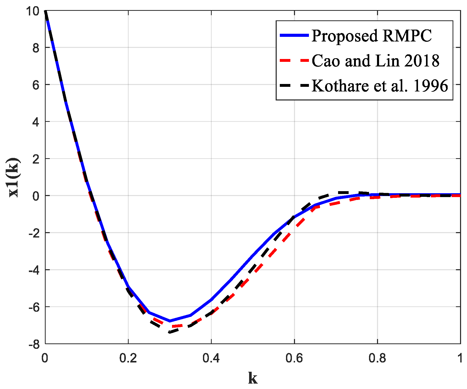
5.1. Example 1

To demonstrate the effectiveness of the proposed RMPC approach, we consider the discrete-time double integrator [58]:

$$x\left(k+1\right)=\left[\begin{array}{cc}1& 1\\ 1& 0\end{array}\right]x\left(k\right)+\left[\begin{array}{c}0\\ 1\end{array}\right]u\left(k\right), y\left(k\right)=\left[\begin{array}{cc}1& 0\end{array}\right]x\left(k\right)$$

which is subject to the input constraint $-1\le u\left(k\right)\le 1$. The discrete-time system starts from the initial condition$x\left(0\right)={\left[\begin{array}{cc}10& -5\end{array}\right]}^T$. We use our saturated RMPC algorithm (Equation (29)) to cope with this problem and compare the results with the saturated RMPC algorithm presented by Cao and Lin [43] and Kothare et al. [37].

Figure 1 shows the state responses and control input of the system under the three different designs. These responses demonstrate that our RMPC guarantees better stabilization performance than that of the previous designs, where the proposed controller results in a smaller overshoot, a shorter rising time, and a faster time response.

Moreover, Figure 2 shows that the accumulated costs associated with the proposed RMPC algorithm is lower than those of the other designs.

5.2. Example 2. DC–DC Buck-Converter-Based PV Pumping System

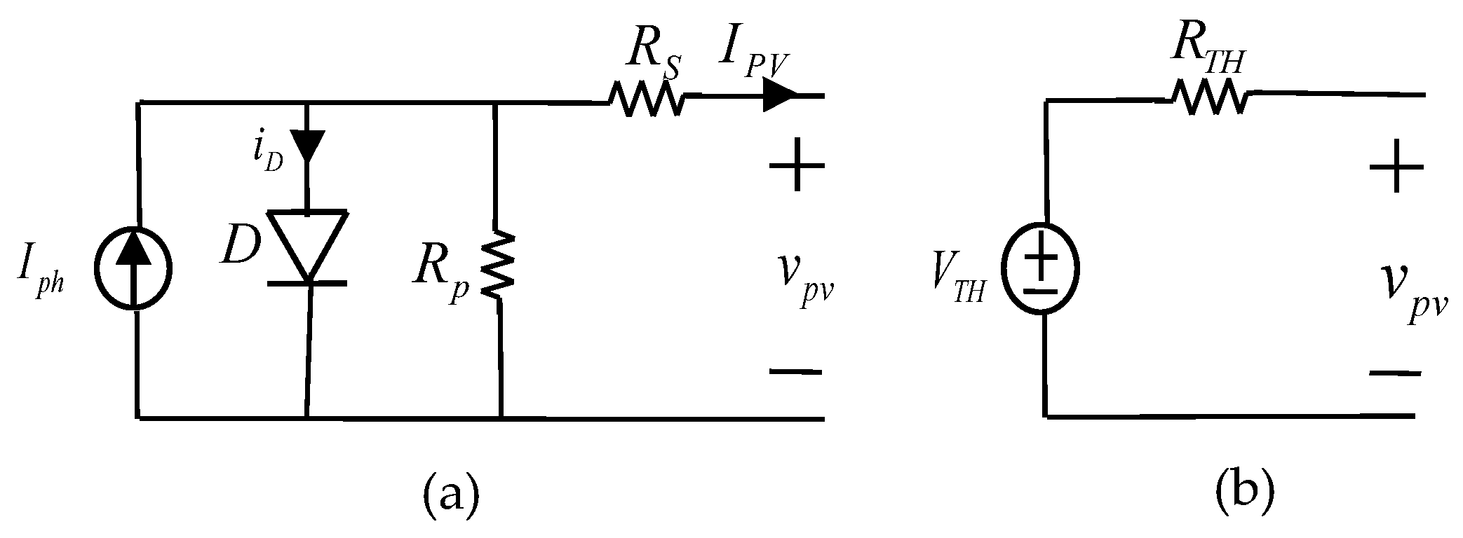
The photovoltaic pumping system under consideration is shown in Figure 3. It comprises a PVG, a DC–DC buck converter, and a DC motor coupled to a centrifugal pump.

5.2.1. PVG Model

Generally, a PVG consists of several solar cells, which are connected in series and parallel to achieve the required voltage and current. The single-diode circuit model in Figure 4a is the most widely used one to study the behavior of a PVG, in which the PVG can be modeled as a current source to model the photo-current $I_{ph}$ in parallel with a diode $D$, an intrinsic shunt resistance $R_P$, and a series resistance$R_S$ (more details can be found in [59,60]). A PVG has a nonlinear voltage–current $\left(V-I\right)$ characteristic (see Figure 5) given by Equation (32), where $v_{pv}$ and $I_{PV}$ are the output voltage and current of the PV module, respectively. The efficiency of PVG depends on the internal characteristics of the device $R_P$ and $R_S$ and on many ambient conditions, such as the solar irradiance level, temperature, and shaded condition.

$$I_{PV}=I_{ph}-I_0\left[exp\left(\frac{v_{pv}+I_{PV}{R}_S}{n{V}_t}\right)-1\right]-\left(\frac{v_{pv}+I_{PV}{R}_S}{R_P}\right)$$

(32)

$I_0$ is the reverse saturation current.

$V_t=\frac{N_{s}KT}{q}$ is the junction thermal voltage of the array with$N_s$ cells connected in series.

$n$ is the ideality factor of the PV cell.

$q=1.60217646\times {10}^{-19} \mathrm{C}$ is the electron charge.

$K=1.3806503\times {10}^{-23}\mathrm{J}/\mathrm{K}$ is the Boltzmann constant.

$\mathrm{T}$ is the temperature in degrees Kelvin.

Since$R_p\gg R_S$, it is possible to assume that $I_{sc}\approx I_{mpp}$. Thus, the photo-current for any temperature and solar irradiation can be expressed by the following equation [61]:

$$I_{ph}=\frac{G_0}{G_{ref}}\left[I_{mpp}+K_i\left(T-T_{ref}\right)\right]$$

(33)

$I_{sc}\mathrm{is}\mathrm{the}$ short-circuit current.

$I_{mpp}$ is the MPP current at STC.

$K_i$ is the short-circuit current temperature coefficient.

$G_0$ is the solar irradiance in$\mathrm{W}/{\mathrm{m}}^2$.

$G_{ref}=1000\mathrm{W}/{\mathrm{m}}^2$ is the solar irradiation reference at STC.

$T_{ref}=25 °\mathrm{C} \left(298\mathrm{degrees}\mathrm{Kelvin}\right)$ is the PVG temperature reference at STC.

The cell reverse saturation current, which depends on temperature, is given by:

$$I_0=I_{rs}{\left[\frac{T}{T_{ref}}\right]}^{3}exp\left[\frac{q{E}_g}{nK}\right]$$

(34)

$I_{rs}$ is the reverse saturation current.

$E_g=1.12\mathrm{eV}$ is the band-gap energy of the semiconductor used in the cell.

$$I_{rs}=\frac{I_{sc,n}}{exp\left(\frac{V_{oc,n}}{n{V}_{t,n}}\right)-1}$$

(35)

$I_{sc,n}$ is the cell short-circuit current at STC.

$V_{oc,n}$is the open-circuit voltage at STC.

$V_{t,n}$ is the junction thermal voltage with$N_s$ cells connected in series at $T_{ref}$.

A modification on the reverse saturation current is proposed in [61] to match the open-circuit voltages of the model with the experimental data (from the manufacturer datasheet) for a wide range of temperatures

$$I_0=\frac{I_{sc,n}+K_i\left(T-T_{ref}\right)}{exp\left[\frac{V_{oc,n}+K_v\left(T-T_{ref}\right)}{n{V}_t}\right]-1}$$

(36)

$K_v$ is the open-circuit voltage temperature coefficient.

The relation between $R_p$ and $R_S$ can be determined by solving Equation (33) for $R_S$ [61]:

$$P_{max}=I_{mpp}{V}_{mpp}=V_{mpp}\left[I_{ph}-I_0\left[exp\left(\frac{q}{KT}\frac{V_{mpp}+I_{mpp}{R}_S}{N_{s}n}\right)-1\right]-\frac{V_{mpp}+I_{mpp}{R}_S}{R_p}\right]$$

(37)

$P_{max}$ is the maximum power from the manufacturer datasheet. Then, $R_p$ can be derived iteratively as:

$$R_p=\frac{V_{mpp}\left(V_{mpp}+I_{mpp}{R}_S\right)}{V_{mpp}{I}_{ph}-V_{mpp}{I}_{0}exp\left[\frac{q\left(V_{mpp}+I_{mpp}{R}_S\right)}{N_{s}nKT}\right]+V_{mpp}{I}_0-P_{max}}$$

(38)

To simplify the PVG model, a Thévenin equivalent circuit shown in Figure 4b can be used, with:

$$R_{TH}=R_S+R_P\parallel R_D$$

(39)

$$V_{TH}=I_{PV}{R}_P$$

(40)

where $V_{TH}$ is Thévenin equivalent voltage and $R_{TH}$ is Thévenin resistance. It can be observed that the Thévenin equivalent circuit parameters are not constant but depend on the environmental variables and operating point.

5.2.2. DC Motor-Pump Model

The DC motor in Figure 3 is a DC motor with a permanent magnet (see Figure 6). This model is defined by an electrical circuit equation armature:

$$v_a\left(t\right)=R_a{i}_a\left(t\right)+e\left(t\right)+L_a\frac{d{i}_a\left(t\right)}{dt}$$

(41)

where $e\left(t\right)$ is the counter electromotive force, $i_a$ is the armature current, $v_a$ is the armature voltage, and $R_a$ and $L_a$ represent the armature resistance and inductance, respectively.

5.2.3. Buck Converter Model

Figure 5 shows the schematic circuit diagram of a PV pumping system formed after connecting a DC motor to a DC–DC buck converter fed from a photovoltaic generator. The converter is assumed to operate in continuous conduction mode (CCM), and the inductor current is always larger than 0. Control is implemented via a pulse width modulation (PWM) approach.$v_{pv}$ is the photovoltaic array voltage, which must be controlled through variation of the duty cycle $d\left(t\right)$ in order to keep the array operation at the maximum power point. The diode$D$ is on inverse polarization, while $C$represents the capacitor value, and $sw$ is a power MOSFET controlled by a binary signal$S_b\left(t\right)$; see Figure 7. The binary signal that triggers the switches on and off is controlled by a fixed-frequency pulse width modulation (PWM) circuit (Figure 7).$1/T_s$ is the constant switching frequency of the PWM circuit, and $T_s$is the switching period given by:

$$T_s=T_{on}+T_{off}$$

(42)

$T_{on}$ is the time when the MOSFET is on $\left(u_b=1\right)$. $T_{off}$ is the time when the MOSFET is off $\left(u_b=0\right)$. The ratio $T_{on}/(T_{on}+T_{off})$ is the duty cycle$d\left(t\right)$. A PWM signal of constant frequency can be obtained by comparing the duty cycle with a sawtooth signal$S_M\left(t\right)$ of amplitude equal to $1$. Consequently, the duty cycle is constrained in amplitude between$0$and $1$:

$$0\le d\left(t\right)\le 1$$

(43)

The average circuit model of the PV pumping system is shown in Figure 8. The corresponding discrete-time model is obtained by using the forward Euler approximation as follows:

$$\begin{array}{l}{i}_a\left(k+1\right)=\left(1-\frac{T_S{R}_a}{L_a}\right)i_a\left(k\right)-\frac{T_S}{L_a}e\left(k\right)+\frac{T_S}{L_a}{v}_{PV}\left(k\right)d \left(k\right)\\ v_{PV}\left(k+1\right)=-\frac{T_S}{C}{i}_a\left(k\right)d\left(k\right)+\left(1-\frac{T_S}{C{R}_{TH}}\right)v_{PV}\left(k\right)+\frac{T_S{V}_{TH}}{R_{TH}}\end{array}$$

(44)

The total instantaneous quantities of the PV system are presented as the sum of the DC and AC components.

$$\begin{array}{l}x\left(k\right)=\tilde{x}\left(k\right)+X\\ d\left(k\right)=\tilde{d}\left(k\right)+D\end{array}$$

(45)

where$x={\left[i_a\left(k\right),v_{pv}\left(k\right)\right]}^T\in {ℝ}^2$ is the state,$d\left(\mathrm{k}\right)\in ℝ$is the saturated control input of the buck converter, $X$ and $D$ represent the equilibrium values, and $\tilde{x}$ and $\tilde{d}$ are the perturbed values of state and input. Using the same concept, we can obtain:

$$\begin{array}{c}{i}_a\left(k\right)=\widetilde{i_a}\left(k\right)+I_a\\ v_{PV}\left(k\right)={\tilde{v}}_{PV}\left(k\right)+V_{PV}\\ d\left(k\right)=H\tilde{x}\left(k\right)+HX\end{array}$$

(46)

Equation (46) is substituted into Equation (44), and a small-signal model is derived as follows:

$$\begin{gathered} \widetilde{i_a}\left(k+1\right)=\left(1-\frac{T_S{R}_a}{L_a}\right)\widetilde{i_a}\left(k\right)-\frac{T_S{V}_{PV}}{L_a}\tilde{d}\left(k\right)+\frac{T_{S }D}{L_a}{\tilde{v}}_{PV}\left(k\right) \\ {\tilde{v}}_{PV}\left(k+1\right)=-\frac{T_S{I}_a}{C}\tilde{d}\left(k\right)-\frac{T_{S}D}{C}\widetilde{i_a}\left(k\right)+\left(1-\frac{T_S}{C{R}_{TH}}\right){\tilde{v}}_{PV}\left(k\right) \end{gathered}$$

(47)

Equation (47) can be expressed as follows:

$$\begin{gathered} x\left(k+1\right)=\tilde{x}\left(k\right)+\dot{X} \\ =A\tilde{x}\left(k\right)+AX+B{}_{\left(0,1\right)}{}^{sat}\left(H\tilde{x}\left(k\right)+HX\right)+\tilde{f}\left(\tilde{x}\left(k\right),\tilde{d}\left(k\right)\right) \end{gathered}$$

(48)

where $\tilde{f}$ is the nonlinear term that is obtained by differing between the nominal nonlinear model and the linear part, given by:

$$\tilde{f}\left(\tilde{x}\left(k\right),\tilde{d}\left(k\right)\right)=f\left(x\left(k\right),d\left(k\right)\right)-A\tilde{x}\left(k\right)+AX+B{}_{\left(0,1\right)}{}^{sat}\left(H\tilde{x}\left(k\right)+HX\right)$$

(49)

And $A=\left[\begin{array}{cc}1-\frac{T_S{R}_a}{L_a}& \frac{T_{S}D}{L_a}\\ -\frac{T_{S}D}{C}& 1-\frac{T_S}{C{R}_{TH}}\end{array}\right],B=\left[\begin{array}{c}\frac{T_S{V}_{PV}}{L_a}\\ -\frac{T_S{I}_a}{C}\end{array}\right]$.

The control input is subject to non-symmetric actuator saturation, and we can use the method proposed in [25] to transform it to a symmetric saturation. Thus, the saturation function of the control input is rewritten as follows:

$${}_{\left(0,1\right)}{}^{sat }\left(H\tilde{x}\left(k\right)+HX\right)=\{\begin{array}{ccc}0,& if& H\tilde{x}\left(k\right)+HX<0\\ H\tilde{x}\left(k\right)+HX& if& 0\le H\tilde{x}\left(k\right)+HX\le 1\\ 1,& if& H\tilde{x}\left(k\right)+HX>1\end{array}$$

(50)

which can be expressed as

$${}_{\left(-HX,1-HX\right)}{}^{sat }\left(K\tilde{x}\left(k\right)\right)=\{\begin{array}{ccc}HX,& if& H\tilde{x}\left(k\right)<-HX\\ H\tilde{x}\left(k\right)& if& HX\le H\tilde{x}\left(k\right)\le 1-HX\\ 1-HX,& if& H\tilde{x}\left(k\right)+HX>1-HX\end{array}$$

(51)

If we add $HX$ to Equation (48), we can obtain the following equality:

$${}_{\left(0,1\right)}{}^{sat }\left(H\tilde{x}\left(k\right)+HX\right)={}_{\left(-HX,1-HX\right)}{}^{sat }\left(H\tilde{x}\left(k\right)\right)+HX$$

(52)

Since the steady-state part is equal to 0, there is:

$$f\left(X,D\right)=AX+HX=0$$

(53)

In our case, the steady-state control signal is $HX=0.5$, and the operating point can be calculated from:

$$\begin{array}{c}{R}_a{I}_a=V_{PV}D \\ D{I}_a=\left(-V_{PV}+V_{TH}\right)/R_{TH}\end{array}$$

(54)

The system described in Equation (48) can be written as follows:

$$\tilde{x}\left(k+1\right)=A\tilde{x}\left(k\right)+Bsat\left(\tilde{\delta }\left(k\right)\right)+\tilde{f}\left(\tilde{x}\left(k\right),\tilde{d}\left(k\right)\right)$$

(55)

where $sat\left(\tilde{\delta }\left(k\right)\right)={}_{\left(-HX,1-HX\right)}{}^{sat}\left(H\tilde{x}\left(k\right)\right)$is the new control input. Lemma 1 can be used to handle saturation nonlinearity. Thus, the new symmetric saturation model is constrained as in [62]:

$$-U_0<u\left(k\right)<U_0\leftrightarrow -HX<\delta \left(k\right)<HX$$

(56)

Based on this amplitude saturation, the decentralized dead-zone nonlinearity can be defined as:

$$\tilde{\phi }\left(k\right)=sat\left(\tilde{\delta }\left(k\right)\right)-\tilde{\delta }\left(k\right)$$

(57)

The closed-loop system is rewritten as:

$$\tilde{x}\left(k+1\right)=\left(A+BH\right)\tilde{x}\left(k\right)+B\tilde{\phi }\left(k\right)+\tilde{f}\left(\tilde{x}\left(k\right),\tilde{d}\left(k\right)\right)$$

(58)

5.2.4. Uncertainty Polytope Model

In this example, the Thévenin resistance $R_{TH}$ at the operating point is considered as the uncertain parameter. The discrete state-space model described in Equation (58) is expressed as:

$$\tilde{x}\left(k+1\right)=\left(A\left(\beta \right)+BH\right)\tilde{x}\left(k\right)+B\tilde{\phi }\left(k\right)+\tilde{f}\left(\tilde{x}\left(k\right),\tilde{d}\left(k\right)\right)$$

(59)

We consider $r=2$ and the vector $\beta \left[1/R_{TH}\right]$, in which:

$$\frac{1}{R_{TH}}\in \left[\frac{1}{R_{THmin}},\frac{1}{R_{THmax}}\right]$$

(60)

Photovoltaic generators are neither constant voltage sources nor constant current sources. In practice, the PVG is forced to operate at the boundaries of the constant current and constant voltage modes, if an MPPT is used, and the possessing dynamic resistance is equal to the resistance of its load at the maximum power transfer [63]. Based on the PVG equivalent circuit of Figure 4b, we can define a range of changes for Thévenin resistance. Under the open-circuit condition, $R_D$ is low, dominating the parallel connection with $R_P$ [15]. Therefore, we have:

$${R_{TH}|}_{oc}\to R_S+R_D$$

(61)

bounded by:

$${R_{TH}|}_{oc}>R_{THmin}=R_S$$

(62)

With short-circuit and reference conditions, $R_D$ is high and $R_P$ dominates the parallel connection. There is:

$${R_{TH}|}_{sc}\to R_P+R_S$$

(63)

Note that $R_S$ is constant and $R_P$ is irradiation dependent [64]:

$$\frac{R_P}{R_{P,ref}}=\frac{G_0}{G_{ref}}$$

(64)

where $G_0$ is the solar irradiance and $R_{P,ref}$ is the shunt resistance at STC (the solar irradiation is $G_{ref}=1000\mathrm{W}/{\mathrm{m}}^2$, and the PVG temperature is$T_{ref}=25°\mathrm{C}$). As an approximation, we have:

$${R_{TH}|}_{sc}<R_{THmax}=R_{P,STC}$$

(65)

Since the PV system matrix $A\left(\beta \right)$ depends linearly on the uncertain parameter$1/R_{TH}$, we can define a polytope of $r=2$vertices, which contains all the possible values of the uncertain matrix. The uncertain matrices $A_j$ are:

$$A_1=\left[\begin{array}{cc}1-\frac{T_S{R}_a}{L_a}& \frac{T_{S}D}{L_a}\\ -\frac{T_{S}D}{C}& 1-\frac{T_S}{C{R}_p}\end{array}\right], A_2=\left[\begin{array}{cc}1-\frac{T_S{R}_a}{L_a}& \frac{T_{S}D}{L_a}\\ -\frac{T_{S}D}{C}& 1-\frac{T_S}{C{R}_S}\end{array}\right]$$

5.2.5. Simulations Results

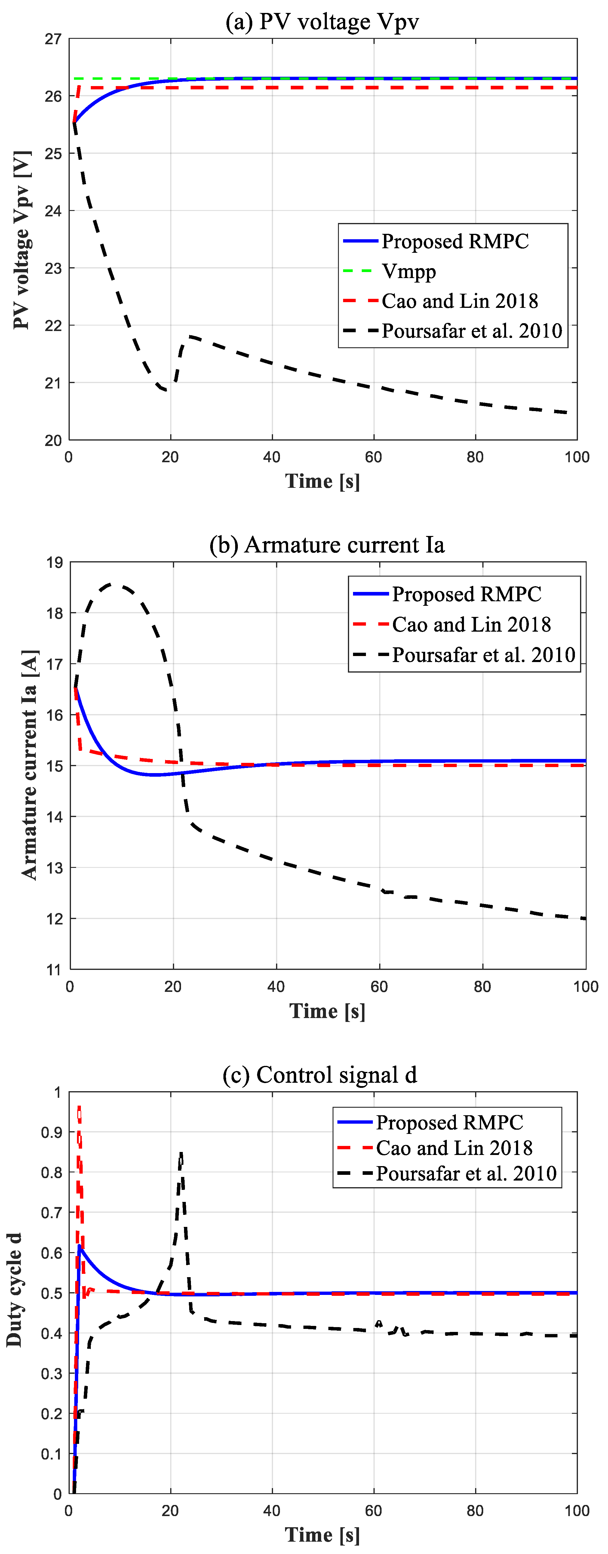
In this section, several simulation tests are implemented to verify the performance of the proposed control law and its robustness according to the presence of the input constraint, insolation variations, temperature variations, and dynamic resistance uncertainty. The results are compared to the RMPC method for nonlinear systems dependent on the Lipschitz bound presented in Poursafar et al. [55] and the saturated RMPC algorithm presented in Cao and Lin [43] designed by the linearized model around the equilibrium point. The parameters of the DC–DC converter and the PVG can be found in

Table 1. Buck converter parameters.

Parameters	Description	Numerical Value
L	Inductance	1 mH
C	Input capacitance	1000 µF
Va	Armature voltage	13.5 V
Ia	Armature current	15.22 A
D	Duty cycle	0.5
Ts	Switching period	0.654 ms

and

Table 2. PVG parameters at STC.

Parameters	Description	Numerical Value
Pmax	Maximum power	200.143 W
Vmpp	Voltage at Pmax	26.3 V
Impp	Current at Pmax	7.61 A
Isc	Short-circuit current	8.21 A
Voc	Open-circuit voltage	32.9 V
KV	Open-circuit voltage temperature coefficient	−0.1230 V/K
Ki	Short-circuit current temperature coefficient	0.0032 A/K
RTH	Thévenin resistance	415.405 Ω
Rs	Series resistance	10 Ω
Rp,STC	Shunt resistance at STC	405.405 Ω

, respectively.

• Scenario 1: The input saturation effect
  In the first case, we assume that the saturation limit is ${\delta }_{max}=0.5$, and the initial conditions of the DC–DC buck converter during startup are represented by $x_0={\left[15.22,26.3\right]}^T$. We use the nominal value of the dynamic resistance $R_{TH}=415.405\mathsf{\Omega }$ to test the closed-loop behavior without any change in the converter parameters. Figure 9 depicts the computed input and state responses under the three different designs, where the waveforms are the PV voltage $v_{pv}$, armature current $i_a$, and duty cycle $d$. From Figure 9, it can be discovered that the proposed method outperforms the saturated RMPC algorithm in Cao and Lin [43] with a fairly good time response and lower fluctuations. Moreover, the PV voltage response settles to its desired value without any overshoot, whereas the approach in [55] has some unstable transient responses. In other words, our RMPC is well capable of handling the hard actuator saturation constraint.
• Scenario 2: The insolation variations effect
  In the second case, we assume that the saturation limit is ${\delta }_{max}=0.5$. An examination is made for various irradiances, such as $G_0=200\mathrm{W}/{\mathrm{m}}^2$, $G_0=400\mathrm{W}/{\mathrm{m}}^2$, and$G_0=1000\mathrm{W}/{\mathrm{m}}^2$. With the proposed control method, the power regulation response is shown in Figure 10. The increasing and decreasing nature of PV power with respect to insolation $G_0$ can be observed in the waveforms of PV power, which verifies the PV generator voltage at the MPP tracking. Similarly, the proposed RMPC also shows a good time response, low oscillation, and desired stability.
• Scenario 3: The temperature variations effect
  In this scenario, we consider varying temperature with constant insolation $G_0=1000\mathrm{W}/{\mathrm{m}}^2$. The temperature changes between $100°\mathrm{K}$ and $298°\mathrm{K}$ at $t=100\mathrm{s}$. Next, the temperature increases to $400°\mathrm{K}$ at $t=200\mathrm{s}$, and it returns to $100°\mathrm{K}$ at $t=300\mathrm{s}$, For this scenario, the saturation limit is ${\delta }_{max}=0.5$. Figure 11 depicts the computed state responses under the proposed RMPC design. It is easily seen that the proposed RMPC guarantees the desired stability, with a good time response and low oscillation.
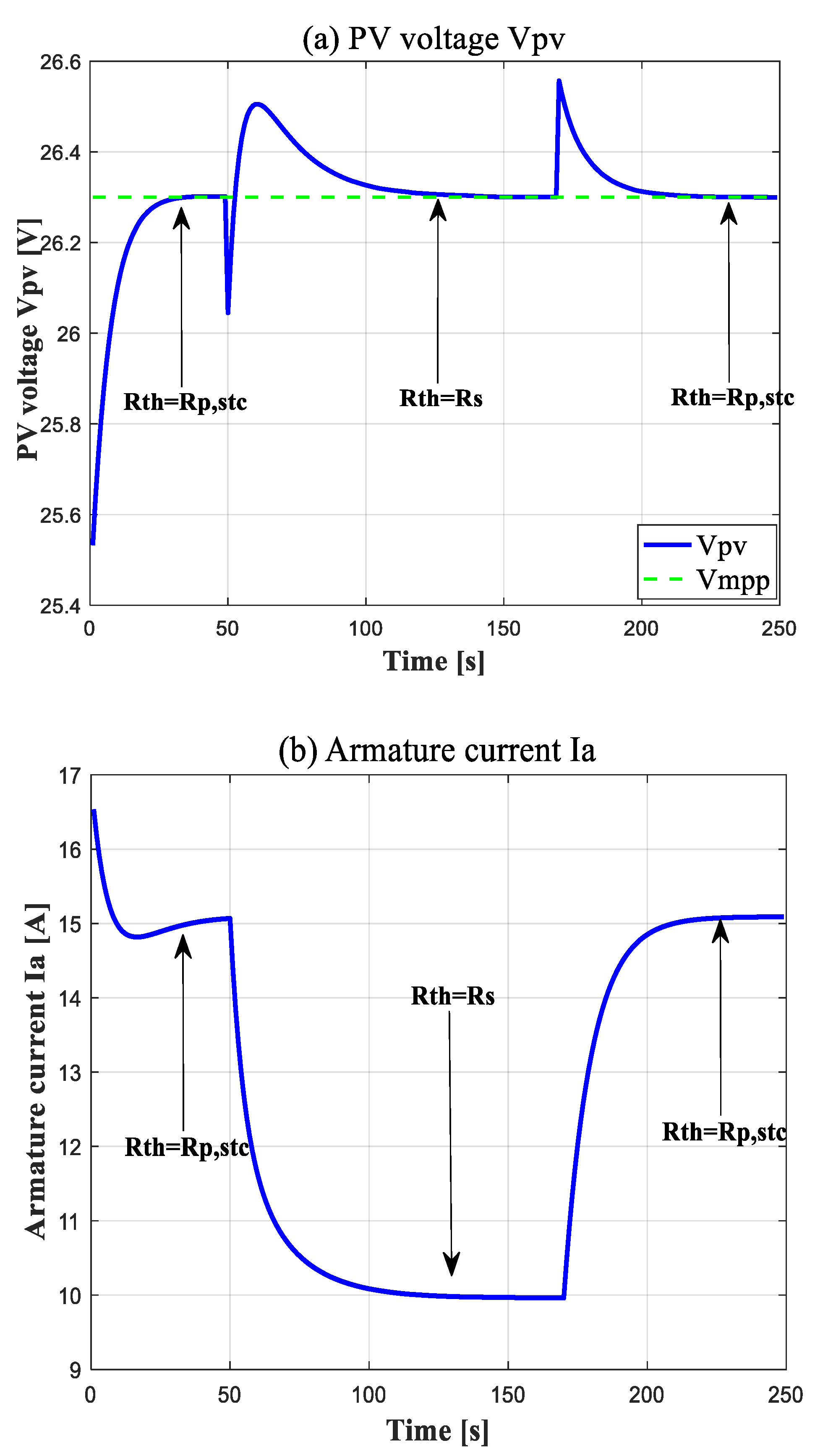
• Scenario 4: The dynamic resistance variations effect
  In the last case, we consider dynamic resistance uncertainty in order to validate the robustness of the proposed controller. Figure 12 illustrates that our controller can stabilize the system on the reference PV voltage in presence of an abrupt dynamic resistance change. The overshoots and long settling time at $t=50\mathrm{s}$and $t=120\mathrm{s}$ are the results of the aggressive move in the converter parameters, which demonstrates the effectiveness of our MPC design algorithm.

6. Conclusions

This paper proposes a new RMPC design framework based on Lyapunov stability theory for a PV pumping system with actuator saturation and uncertain parameters. The input saturation effect is expressed by a model using dead-zone nonlinearity. At each time instant, the state feedback control law is obtained by minimizing the upper bound of the infinite horizon cost function within the framework of LMIs, which directly incorporates the input saturation. The internal stability of the closed-loop system is guaranteed in the sense of Lyapunov stability. The design of the closed-loop stabilization for a nonlinear system for the requirement of desired output responses with uncertain parameters is also investigated here. The simulation results obtained demonstrate the effectiveness and efficiency of our method. Furthermore, the novel method is examined in case the uncertainty is in the form of solar irradiance change and dynamic resistance, which proves that it is able to stabilize the system at the desired PV voltage.

References

1. Cui, W.; Li, X.; Li, X.; Si, T.; Lu, L.; Ma, T.; Wang, Q. Thermal performance of modified melamine foam/graphene/paraffin wax composite phase change materials for solar-thermal energy conversion and storage. J. Clean. Prod. 2022, 367, 133031. [Google Scholar] [CrossRef]
2. Joshi, S.; Karamta, M.; Pandya, B. Small scale wind & solar photovoltaic energy conversion system for DC microgrid applications. Mater. Today Proc. 2022, 62, 7092–7097. [Google Scholar]
3. Mura, P.G.; Baccoli, R.; Innamorati, R.; Mariotti, S. Solar energy system in a small town constituted of a network of photovoltaic collectors to produce Electricity for homes and hydrogen for transport services of municipality. Energy Procedia 2015, 78, 824–829. [Google Scholar] [CrossRef] [Green Version]
4. Mura, P.G.; Baccoli, R.; Innamorati, R.; Mariotti, S. An energy autonomous house equipped with a solar PV hydrogen conversion system. Energy Procedia 2015, 78, 1998–2003. [Google Scholar] [CrossRef] [Green Version]
5. Alvear-Daza, J.J.; Sanabria, J.; Gutiérrez-Zapata, H.M.; Rengifo-Herrera, J.A. An integrated drinking water production system to remove chemical and microbiological pollution from natural groundwater by a coupled prototype helio-photochemical/H2O2/rapid sand filtration/chlorination powered by photovoltaic cell. Sol. Energy 2018, 176, 581–588. [Google Scholar] [CrossRef]
6. Ren, F.-R.; Tian, Z.; Liu, J.; Shen, Y.-T. Analysis of CO2 emission reduction contribution and efficiency of China’s solar photovoltaic industry: Based on Input-output perspective. Energy 2020, 199, 117493. [Google Scholar] [CrossRef]
7. Siddiqui, O.; Ishaq, H.; Chehade, G.; Dincer, I. Experimental investigation of an integrated solar powered clean hydrogen to ammonia synthesis system. Appl. Therm. Eng. 2020, 176, 115443. [Google Scholar] [CrossRef]
8. Maranhao, G.N.; Brito, A.U.; Pinho, J.T.; Fonseca, J.K.S.; Leal, A.M.; Macedo, W.N. Experimental Results of a Fuzzy Controlled Variable-Speed Drive for Photovoltaic Pumping Systems. IEEE Sens. J. 2016, 16, 2854–2864. [Google Scholar] [CrossRef]
9. Ghosh, A.; Malla, S.G.; Bhende, C.N. Small-signal modelling and control of photovoltaic based water pumping system. ISA Trans. 2015, 57, 382–389. [Google Scholar] [CrossRef]
10. Mishra, A.K.; Singh, B. Solar photovoltaic array dependent dual output converter based water pumping using Switched Reluctance Motor drive. IEEE Trans. Ind. Appl. 2017, 53, 5615–5623. [Google Scholar] [CrossRef]
11. Rajan, K.; Bhim, S. Single Stage Solar PV Fed Brushless DC Motor Driven Water Pump. IEEE J. Emerg. Sel. Top. Power Electron. 2017, 5, 1377–1385. [Google Scholar]
12. Kolhe, M.; Joshi, J.; Kothari, D. Performance Analysis of a Directly Coupled Photovoltaic Water-Pumping System. IEEE Trans. Energy Convers. 2004, 19, 613–618. [Google Scholar] [CrossRef]
13. Elgendy, M.A.; Zahawi, B.; Atkinson, D.J. Comparison of Directly Connected and Constant Voltage Controlled Photovoltaic Pumping Systems. IEEE Trans. Energy Convers. 2010, 1, 184–192. [Google Scholar] [CrossRef]
14. Elgendy, M.A.; Zahawi, B.; Atkinson, D.J. Assessment of Perturb and Observe MPPT Algorithm Implementation Techniques for PV Pumping Applications. IEEE Trans. Energy Convers. 2012, 3, 21–33. [Google Scholar] [CrossRef]
15. Sitbon, M.; Schacham, S.; Kuperman, A. Disturbance Observer Based Voltage Regulation of Current-Mode-Boost-Converter-Interfaced Photovoltaic Generator. IEEE Trans. Ind. Electron. 2015, 62, 5776–5785. [Google Scholar] [CrossRef]
16. Salas, V.; Barrado, A. Review of the maximum power point tracking algorithms for stand-alone photovoltaic systems. Sol. Energy Mater. Sol. Cells 2006, 90, 1555–1578. [Google Scholar] [CrossRef]
17. Femia, N.; Petrone, G.; Spagnuolo, G.; Vitelli, M. Optimization of perturb and observe maximum power point tracking method. IEEE Trans. Power Electron. 2005, 20, 963–973. [Google Scholar] [CrossRef]
18. Zegaoui, A.; Aillerie, M.; Petit, P.; Sawicki, J.P.; Jaafar, A.; Salame, C.; Charles, J.P. Comparison of two common maximum power point trackers by simulating of PV generators. Energy Proc. 2011, 6, 678–687. [Google Scholar] [CrossRef]
19. Kadri, R.; Gaubert, J.; Champenois, G. An improved maximum power point tracking for photovoltaic grid-connected inverter based on voltage oriented control. IEEE Trans. Ind. Electron. 2011, 58, 66–75. [Google Scholar] [CrossRef]
20. Leppaaho, J.; Huusari, J.; Nousiainen, L.; Puukko, J.; Suntio, T. Dynamic properties and stability assessment of current fed converters in photovoltaic applications. IEEE Trans. Ind. Appl. 2011, 131, 976–984. [Google Scholar] [CrossRef]
21. Suntio, T.; Viinamaki, J.; Jokipii, J.; Messo, T.; Kuperman, A. Dynamic characterization of power electronics interfaces. IEEE J. Emerg. Sel. Top. Power Electron. 2014, 2, 949–961. [Google Scholar] [CrossRef]
22. Middlebrook, R.D.; Cuk, S. A general unified approach to modelling switching-converters. Int. J. Electron. 1977, 42, 521–550. [Google Scholar] [CrossRef]
23. Perry, A.G.; Feng, G.; Liu, Y.F.; Sen, P.C. A design method for PI-like fuzzy logic controllers for DC–DC converter. IEEE Trans. Ind. Electron. 2007, 54, 2688–2696. [Google Scholar] [CrossRef]
24. Shirazi, M.; Zane, R.; Maksimovic, D. An Autotuning Digital Controller for DC–DC Power Converters Based on Online Frequency-Response Measurement. IEEE Trans. Power Electron. 2009, 24, 2578–2588. [Google Scholar] [CrossRef]
25. Olalla, C.; Queinnec, I.; Leyva, R.; El Aroudi, A. Robust optimal control of bilinear DC-DC converters. Control. Eng. Pract. 2011, 19, 688–699. [Google Scholar] [CrossRef]
26. Emadi, A.; Khaligh, A.; Rivetta, C.; Williamson, G. Constant power loads and negative impedance instability in automotive systems: Definition, modeling, stability, and control of power electronic converters and motor drives. IEEE Trans. Veh. 2006, 55, 1112–1125. [Google Scholar] [CrossRef]
27. Li, X.; Wen, H.; Hu, Y.; Jiang, L. A novel beta parameter based fuzzy-logic controller for photovoltaic MPPT application. Renew. Energy 2019, 130, 416–427. [Google Scholar] [CrossRef]
28. Youssefa, A.; El Telbanya, M.; Zekry, A. Reconfigurable generic FPGA implementation of fuzzy logic controller for MPPT of PV systems. Renew. Sustain. Energy Rev. 2018, 82, 1313–1319. [Google Scholar] [CrossRef]
29. Chan, C.-Y.; Chincholkar, S.H.; Zekry, W. Adaptive Current-Mode Control of a High Step-Up DC-DC Converter. IEEE Trans. Power Electron. 2017, 32, 7297–7305. [Google Scholar] [CrossRef]
30. Zheng, S.; Li, W. Adaptive control for switched nonlinear systems with coupled input nonlinearities and state constraints. Inf. Sci. 2018, 462, 331–356. [Google Scholar] [CrossRef]
31. Yu, J.; Chen, B.; Yu, H.; Lin, C.; Zhao, L. Neural networks-based command filtering control of nonlinear systems with uncertain disturbance. Inf. Sci. 2018, 426, 50–60. [Google Scholar] [CrossRef]
32. Tian, Z.; Lyu, Z.; Wang, C. UDE-based sliding mode control of DC–DC power converters with uncertainties. Inf. Sci. 2019, 83, 116–128. [Google Scholar] [CrossRef]
33. Jinbo, L.; Wenlong, M. A new experimental study of input-output feedback linearization based control of boost type DC/DC converter. In Proceedings of the IEEE International Conference on Industrial Technology, Via del Mar, Chile, 14–17 March 2010; pp. 685–689. [Google Scholar]
34. Ghaffari, V.; Vahid Naghavi, S.; Safavi, A.A. Robust model predictive control of a class of uncertain nonlinear systems with application to typical CSTR problems. Proc. Am. Control. Conf. 2013, 23, 493–499. [Google Scholar] [CrossRef]
35. Bououden, S.; Allouani, F.; Abboudi, A.; Chadli, M.; Boulkaibet, I.; Al Barakeh, Z.; Neji, B.; Ghandour, R. Observer-Based Robust Fault Predictive Control for Wind Turbine Time-Delay Systems with Sensor and Actuator Faults. Energies 2023, 16, 858. [Google Scholar] [CrossRef]
36. Qin, S.J.; Badgwell, T.A. A survey of industrial model predictive control technology. Control Eng. Pract. 2003, 11, 733–764. [Google Scholar] [CrossRef]
37. Kothare, M.V.; Balakrishnan, V.; Morari, M. Robust Constrained Model Predictive Control Using Linear Matrix Inequalities. Automatica 1996, 32, 1361–1379. [Google Scholar] [CrossRef] [Green Version]
38. Casavola, A.; Giannelli, M.; Mosca, E. Min–max predictive control strategies for input-saturated polytopic uncertain systems. Automatica 2000, 36, 125–133. [Google Scholar] [CrossRef]
39. Angeli, D.; Casavola, A.; Franzč, G.; Mosca, E. An ellip soidal off-line MPC scheme for uncertain polytopic discrete-time systems. Automatica 2008, 44, 3113–3119. [Google Scholar] [CrossRef]
40. Cheng, X.; Jia, D. Robust stability constrained model predictive control. In Proceedings of the American Control Conference, Boston, MA, USA, 30 June–2 July 2004; pp. 1580–1585. [Google Scholar]
41. Alamo, T.; Cepeda, A.; Limon, D.; Camacho, E.F. Estimation of the domain of attraction for saturated discrete-time systems’. Int. J. Syst. Sci. 2010, 37, 575–583. [Google Scholar] [CrossRef]
42. Hu, T.; Lin, Z. Control systems with actuator saturation: Analysis and design. In Birkhäuser, 1st ed.; Springer: Boston, MA, USA, 2001; pp. 327–373. [Google Scholar]
43. Cao, Y.Y.; Lin, Z. Min–max MPC algorithm for LPV systems subject to input saturation. IEE Proc. Control. Theory Appl. 2018, 152, 266–272. [Google Scholar] [CrossRef]
44. Huang, H.; Li, D.; Lin, Z.; Xi, Y. An improved robust model predictive control design in the presence of actuator saturation. Automatica 2011, 47, 861–864. [Google Scholar] [CrossRef]
45. Zabiri, H.; Samyudia, Y. A hybrid formulation and design of model predictive control for systems under actuator saturation and backlash. J. Process Control. 2006, 16, 693–709. [Google Scholar] [CrossRef]
46. Besselmann, T.; Lofberg, J.; Morari, M. Explicit MPC for LPV Systems: Stability and Optimality. IEEE Trans. Autom. Control 2012, 57, 2322–2332. [Google Scholar] [CrossRef] [Green Version]
47. Yu, S.; Bohm, C.; Chen, H.; Allgower, F. Stabilizing model predictive control for LPV systems subject to constraints with parameter-dependent control law. In Proceedings of the 2009 Conference on American Control Conference, St. Louis, MO, USA, 10–12 June 2009; pp. 3118–3123. [Google Scholar]
48. Zhang, L.; Wang, J.; Li, C. Distributed model predictive control for polytopic uncertain systems subject to actuator saturation. J. Process Control 2013, 23, 1075–1089. [Google Scholar] [CrossRef]
49. Guo, M.; Wang, D. Guidance law for low-lift skip reentry subject to control saturation based on nonlinear predictive control. Aerosp. Sci. Technol. 2014, 37, 48–54. [Google Scholar]
50. Weiwei, Q.; Bing, H.; Gang, L.; Pengtao, Z. Robust model predictive tracking control of hypersonic vehicles in the presence of actuator constraints and input delays. J. Frankl. Inst. 2016, 353, 4351–4367. [Google Scholar] [CrossRef]
51. Peng, H.; Li, F.; Zhang, S.; Chen, B. A novel fast model predictive control with actuator saturation for large-scale structures. Comput. Struct. 2017, 187, 35–49. [Google Scholar] [CrossRef] [Green Version]
52. Yu, S.; Qu, T.; Xu, F.; Chen, H.; Hu, Y. Stability of finite horizon model predictive control with incremental input constraints. Automatica 2017, 79, 265–272. [Google Scholar] [CrossRef]
53. Galuppini, G.; Magni, L.; Martino Raimondo, D. Model predictive control of systems with dead zone and saturation. Control Eng. Pract. 2018, 78, 56–64. [Google Scholar] [CrossRef]
54. Li, X.; Sun, G.; Shao, X. Discrete-time pure-tension sliding mode predictive control for the deployment of space tethered satellite with input saturation. Acta Astronaut. 2020, 170, 521–529. [Google Scholar] [CrossRef]
55. Poursafar, N.; Taghirad, H.D.; Haeri, M. Model predictive control of non-linear discrete time systems: A linear matrix inequality approach. IET Control Theory Appl. 2010, 4, 1922–1932. [Google Scholar] [CrossRef]
56. Sun, L.; Wangn, Y.; Feng, G. Control design for a class of affine nonlinear descriptor systems with actuator saturation. IEEE Trans. Autom. Control 2015, 60, 2195–2200. [Google Scholar] [CrossRef]
57. Boyd, S.; El Ghaoui, L.; Feron, E.; Balakrishnan, V. Linear matrix inequalities in systems and control theory. In Studies in Applied and Numerical Mathematics; SIAM: Philadelphia, PA, USA, 1994; Volume 1562, pp. 5776–5785. [Google Scholar]
58. Lu, Y.; Arkun, Y. A quasi-min-max MPC algorithms for linear parameter varying systems with bounded rate of change of parameters. In Proceedings of the 2000 American Control Conference. ACC, Chicago, IL, USA, 28–30 June 2000; Volume 5, pp. 3234–3238. [Google Scholar]
59. Izadian, A.; Pourtaherian, A.; Motahari, S. Basic Model and Governing Equation of Solar Cells used in Power and Control Applications. In Proceedings of the 2012 IEEE Energy Conversion Congress and Exposition (ECCE), Raleigh, NC, USA, 15–20 September 2012; pp. 1483–1488. [Google Scholar]
60. Ortiz-Conde, A.; Lugo-Munoz, D.; Garcia-Sanchez, J. An explicit Multi exponential Model as an Alternative to Traditional Solar Cell Models with Series and Shunt Resistances. IEEE J. Photovolt. 2012, 2, 261–268. [Google Scholar] [CrossRef]
61. Villalva, M.G.; Gazoli, J.R.; Filho, E.R. Comprehensive Approach to Modeling and Simulation of Photovoltaic Arrays. IEEE Trans. Power Electron. 2009, 24, 1198–1208. [Google Scholar] [CrossRef]
62. Gomes da Silva, J.; Tarbouriech, S. Anti-windup design with guaranteed regions of stability: An lmi-based approach. IEEE Trans. 2005, 50, 106–111. [Google Scholar]
63. Nakanishi, F.; Ikegami, T.; Ebihara, K.; Kuriyama, S.; Shiota, Y. Modeling and Operation of a 10 kW Photovoltaic Power Generator Using Equivalent Electric Circuit Method. In Proceedings of the IEEE Photovoltaic Specialists Conference, Anchorage, AK, USA, 15–22 September 2000; 2000. [Google Scholar]
64. Tian, H.; Mancilla-David, F.; Ellis, K.; Muljadi, E.; Jenkins, P. A cell-to-module-to-array detailed model for photovoltaic panels. Sol. Energy 2012, 86, 2695–2706. [Google Scholar] [CrossRef]
Figure 1. State responses and control input [37,43].
Sustainability 15 04493 g001aSustainability 15 04493 g001b
Figure 2. Accumulated costs [37,43].
Sustainability 15 04493 g002
Figure 3. Proposed PV pumping system block diagram.
Sustainability 15 04493 g003
Figure 4. Equivalent electrical scheme of the PVG: (a) detailed and (b) Thévenin.
Sustainability 15 04493 g004
Figure 5. PVG I–V curve.
Sustainability 15 04493 g005
Figure 6. Equivalent electrical scheme of the PV pumping system with the RMPC.
Sustainability 15 04493 g006
Figure 7. PWM waveforms.
Sustainability 15 04493 g007
Figure 8. Averaged circuit model of PV pumping system.
Sustainability 15 04493 g008
Figure 9. Simulated transient of the buck converter under saturation constraint | δ m a x | 0.5 : (a) PV voltage V p v , (b) armature current   I a , and (c) control signal d .
Sustainability 15 04493 g009
Figure 10. Simulated transient of the buck converter with varying insolation: (a) PV voltage V p v and (b) armature current   I a .
Sustainability 15 04493 g010
Figure 11. Simulated transient of the buck converter with varying temperature: (a) PV voltage V p v and (b) armature current   I a .
Sustainability 15 04493 g011
Figure 12. Simulated transient of the buck converter under a dynamic resistance step transient [ R T H = R P , S T C R S R P , S T C ] : (a) PV voltage V p v and (b) armature current   I a .
Sustainability 15 04493 g012