Life Cycle Assessment of Greenhouse Gas Emissions from Recycled Asphalt Pavement Production

Abstract

With the growing impact of climate change, there is an increasing need and obligation to reduce the responsible greenhouse gases (GHG) in road construction as well. Using life cycle assessment (LCA) methods, several studies have already separately analysed individual parameters of the asphalt production process and illustrated potential improvements in terms of GHG reduction. However, the data of most assessments originate from single sources and databases, and as such can offer little validation against unreliable assumptions. For this reason, in addition to conducting separate assessments at quarries, batch asphalt mixing plants, and construction sites in order to collect energy and material consumption data with which to calculate GHG emissions, this work relies on the results of multiple sources found in the literature. Using the structure for environmental product declarations (EPDs) in EN 15804, our results are divided into the different stages of a life cycle and the corresponding modules. This allows for systematic comparison of different products and eliminates previous uncertainties regarding the inclusion of benefits beyond the system boundary. The results show the dominance of asphalt binder in the material footprint and the corresponding advantage of substituting virgin material with recycled material, as well as the influence of material moisture on GHG emissions in the production process. In addition to the evaluating the material itself, two road sections with increasing traffic volume (and increasing share of electric mobility) were examined and compared with the traffic-related GHG emissions over a 30-year lifetime. We can confirm that traffic has a substantially higher share of the total GHG emissions (>95%); however, as its regulation is the responsibility of governments, the construction industry can only bring about improvements in its own sphere in seeking to further climate protection.

1. Introduction

With the increasing impact of climate change, the reduction of greenhouse gas (GHG) emissions is becoming increasingly important on a global scale. Road infrastructure is particularly vulnerable to the consequences of climate change, such as severe weather and extreme temperatures, as it was not originally designed with these factors in mind. It is therefore crucial to identify the factors in the road infrastructure production chain that contribute to climate change and to find ways to reduce the environmental impact of these materials. One approach to achieve this is to use life cycle assessment (LCA) methods, which provide a structured way to compare the production of road pavements under different boundary conditions.

Many LCA studies have been conducted to date, most of them specialised on certain aspects of the production, construction, or use stage of asphalt pavements [1,2,3,4,5,6,7]. For the production stage, which is dominated by the energy demand for heating and drying of materials, a substantial reduction of GHG emissions is possible when using dry aggregates and natural gas [8]. In particular, the influence of moist aggregates on the energy demand is quite high, ranging from 7 to 8 kWh/t asphalt pavement per 1% increase of moisture content [9,10]. A practical study has found that the calculated theoretical energy demand used in most literature exceeds the actual energy consumption by 11 to 13% [9].

Another factor in reducing energy demand and GHG emissions is lowering the production temperature, which can lead to energy savings of 2.6 kWh/t asphalt pavement per 10 °C decrease (between 150 °C and 200 °C asphalt pavement temperature) [10]. A more drastic measure to reduce production temperatures is using warm mix asphalt (in general <150 °C), which reduces energy demand and emissions (not only GHG emissions) [11]; however, the consequent use of the necessary additives may offset this advantage [12]. A combination of reduced temperatures and reclaimed asphalt pavement (RAP) added in the range of 10–50% has proven to be beneficial for GHG emissions, with a decrease of 12–17%. The primary advantage of RAP is the reduction in the amount of virgin materials (especially asphalt binder) required for production [12,13,14]. In contrast to Austria, countries with low resources of qualitatively suitable aggregates must use RAP or recycled aggregates (RCA) to avoid long-distance transport of virgin aggregates. This can make the use of RAP/RCA even more beneficial, as in certain cases GHG emissions are reduced by up to 65% when using RCA compared to virgin material [15]. It should be noted that RAP should be preferred solely in asphalt pavements due to its binder content; RCA, on the other hand can replace virgin aggregate in both asphalt pavements and in concrete pavements and subgrade layers.

In addition to asphalt binder having a large carbon footprint in general, quite large differences in energy demand, and consequently GHG emissions, are observed due to the different system boundaries, technological efficiencies, and regulations in different countries [16]. A reduction in GHG emissions of up to 8% can be achieved by replacing 10% of virgin binder with bio-based binders [17].

A more holistic view of road systems shows that the use stage with traffic cannot be neglected over a certain lifetime, as traffic-related GHG emissions are more than 1000 times higher than the sum of production, construction, and rehabilitation [14]. The urgency of reducing GHG emissions is even clearer when additionally accounting for faster deterioration of roads due to climate change, primarily higher temperatures. This may lead to more road rehabilitation work being required, which, when combined with traffic, leads to higher fuel consumption due to increased road roughness [18].

The use of individual databases to assess the effect of specific processes and materials on GHG emissions has been performed in many studies presented to date. While this is common, it makes the results vulnerable to false assumptions and uncertainties in these values. For example, high variance has been found in on-site emission measurements, with CO and CH₄ emissions particularly affected (CH₄ is a GHG), mainly because they both depend on the combustion efficiency of gas burners [19]. Therefore, relying on single sources can be problematic. The present work mitigates this problem by using multiple sources and using the structure for environmental product declarations (EPD) according to EN 15804 [20]. This ensures better comparability of products and processes under different boundary conditions by clearly dividing the results into the stages and corresponding modules (see Section 2.2), which additionally removes uncertainties with respect to the allocation and especially the inclusion of benefits beyond the system boundary.

Hence, the aim of this study is to: (i) investigate the GHG emissions of the asphalt pavement production, (ii) the extent to which different factors are influential during production, and (iii) the comparison of GHG emissions during a 30-year lifetime (according to Austrian regulations [21]) of asphalt pavements, including rehabilitation works, in both a low traffic volume and a high traffic volume road section. The results provide information on the environmental impact of common road materials, and in particular provide clarification about how different settings of the asphalt production process (moisture of aggregates, adding RAP, etc.) influence energy demand and GHG emissions.

2. Materials and Methods

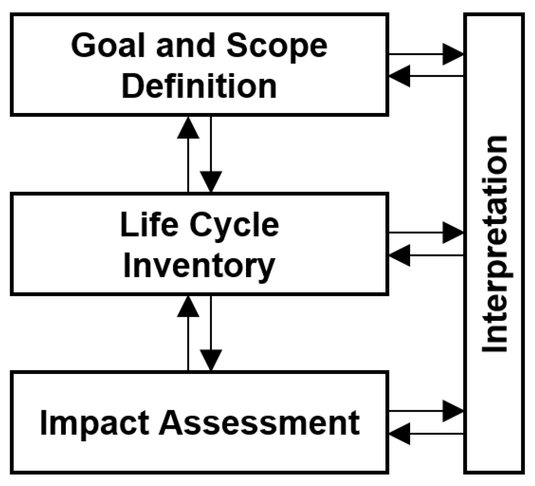
To assess the environmental impact of processes and products, we conducted an LCA based on the standard ISO 14040 and consisting of the following main modules: goal and scope definition, inventory analysis, impact assessment, and interpretation of results, as shown in Figure 1 [22]. The following subsections provide an overview of which processes are included for the production of one ton of asphalt pavement.

2.1. LCA—Goals and Scope

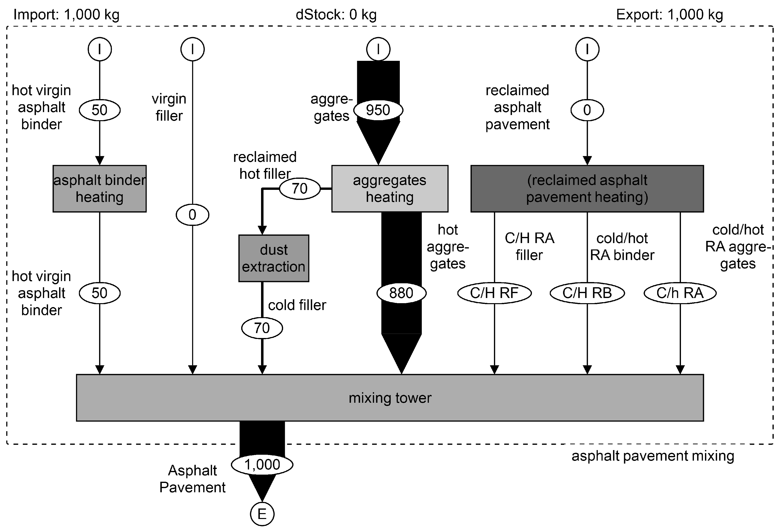
The aim of this first part is to investigate the GHG emissions of the asphalt pavement production and their influencing factors. The system boundaries, include materials and energy inputs and outputs, are shown for asphalt production in Figure 2, illustrating the options for adding hot or cold RAP. This material flow analysis was performed using STAN software (https://www.stan2web.net/, accessed on 1 March 2023) [23]. The inputs were as follows:

• hot virgin asphalt binder (delivered hot);
• virgin filler (produced when drying aggregates—see Section 3.3);
• virgin mineral aggregates;
• RAP.

The materials and energy input for the production of mixing plants, trucks etc., or wear and tear of used products was not taken into account. One ton (=1000 kg) was used as functional unit; wherever possible, data originating from Europe were preferred. To ensure good structure and clarity, the results were divided into modules according to EN 15804.

There are a total of 24 indicators for an LCA according to EN 15804+A2:2019 (compared to seven indicators in EN 15804:2012). These are divided into the categories of environmental impact, resource use, waste and output flows. The first category, environmental impact, consists of thirteen indicators: climate change (total, fossil, biogenic, LULUC), ozone depletion, acidification, eutrophication (aquatic freshwater, aquatic marine, terrestrial), photochemical ozone formation, abiotic depletion (minerals and metals, fossil resources), and water use. Additionally, there are other categories, e.g., resource use, waste, and output flows; however, this study only concentrates on the global warming potential GWP (now: climate change total) as expressed by GHG emission in kg CO₂-equivalents per ton of asphalt pavement (kg CO₂e/t).

2.2. LCA—Modules

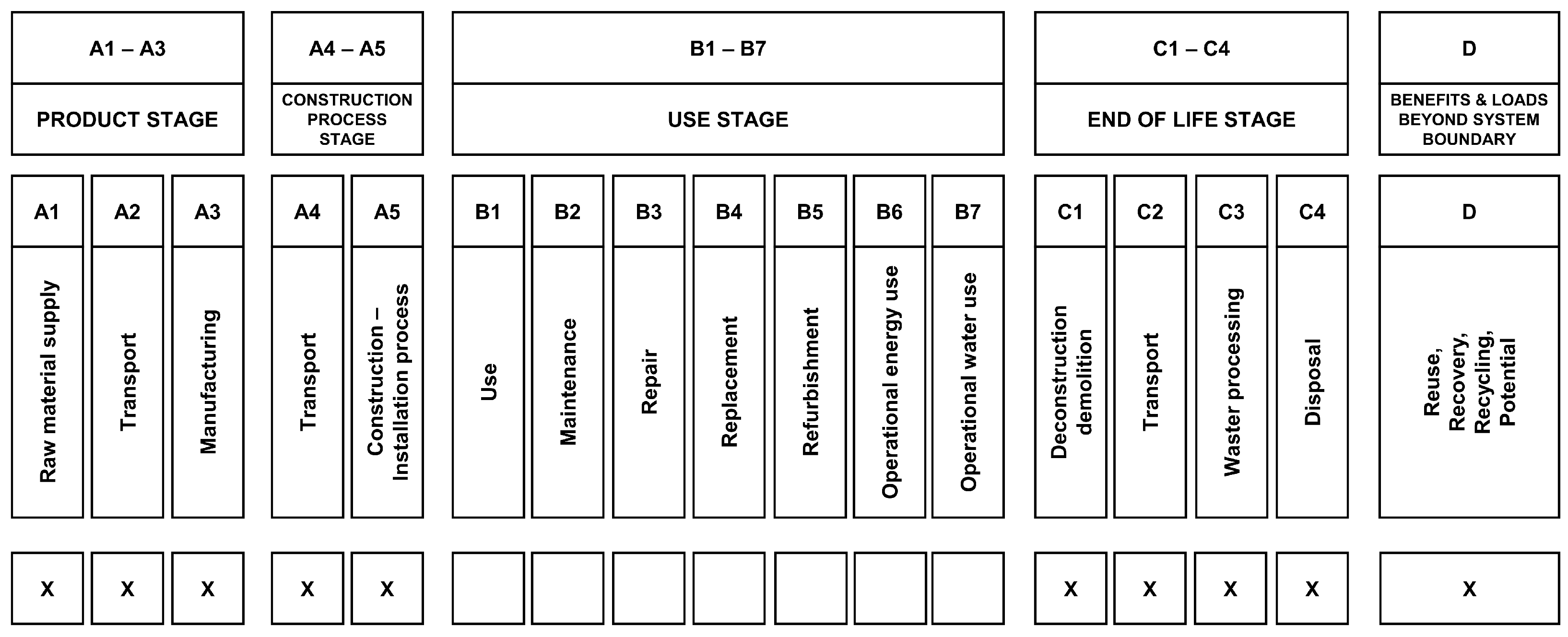
To standardise EPDs, each step in the life cycle of a product can be summarised in a stage consisting of different modules. For instance, the product stage (A1–A3) is a combination of the modules raw material supply (A1), transport (A2), and manufacturing (A3). A summary of all stages and modules, which in this work include modules A1–A5, C1–C4, and D (marked with x), can be found in Figure 3.

3. Results and Discussion

3.1. Module A1—Raw Material Supply

The following subsections provide information on how much GHG emissions must be associated with base materials of asphalt pavements, i.e., mineral aggregates (coarse, fine) and asphalt binder.

3.1.1. Module A1—Mineral Aggregate Production in Quarry

This module section is part of the module raw material supply (A1) of the asphalt production, and represents a cradle-to-gate approach for mineral aggregates. Processes include drilling holes for explosives, blasting, internal transport, crushing, and screening to make the product (mineral aggregate in different sizes) ready for sale.

Data collection for coarse mineral aggregates was divided into measured data from quarries and data from the literature. Because the former data represent the actual use of resources for these activities, they were further used to calculate emissions, while data from the literature were only used to validate the data collected from quarries.

Data from Quarries

Three quarries supplied the consumed amount of diesel and electricity, explosives (ammonium nitrate and fuel oil, or ANFO), fuel oil, and water for up to five years for the production of mineral aggregates (see

Table A1. Materials—production of coarse mineral aggregate in quarry.

Type	ANFO	Elect.	Diesel	Heating Oil	Liq. Gas	Water
Unit	kg/t	kWh/t	L/t	L/t	L/t	L/t
n	7	10	10	4	4	2
Mean	0.06	3.09	0.51	0.021	0.003	0.001
SD	0.01	1.05	0.07	0.001	0.000	0.000

in the Appendix A). All these energy resources produce emissions while being used or when being produced; hence, we multiplied the resource’s emission factor by the amount used (see Table A1), resulting to obtain the GHG emissions of 2.51 kg CO₂e per ton of mineral aggregate, which is shown in

Table 1. GHG—production of coarse mineral aggregates in quarry.

Type	ANFO	Elect.	Diesel	Heat. Oil	Liq. Gas	Water	Total
Unit	kg CO2e/t
n	7	10	10	4	4	2	-
Mean	0.14	0.68	1.62	0.069	0.01	0.00	2.51
SD	0.03	0.23	0.23	0.004	0.00	0.00	0.49
Share	5.55%	26.99%	64.42%	2.74%	0.30%	0.01%	100%

.

Data from the Literature

The mineral processing industry has published EPDs in many European countries, and as such is already a step further ahead than construction industries in other jurisdictions. In addition to these EPDs, the GHG emissions can be extracted from various databases, such as e.g., Ecoinvent, ProBas, or Oekobaudat. The crushing of aggregates produces fine aggregates such as sand; however, sand is often extracted from quarry ponds, which may explain the difference in GHG emissions from the production of fine mineral aggregates.

The mean value for coarse mineral aggregates is 2.79 kg CO₂e per ton, while for fine mineral aggregates (0/2 and 0/4 fraction) it is 2.06 kg CO₂e per ton. Detailed calculations can be found in the

Table A2. GHG—production of coarse mineral aggregate in quarry.

Type	Source	URL (accessed on 1 March 2023)	kg CO2e/t
Gravel 2/32	Oekobaudat (CSV)	https://tinyurl.com/yc5vazr9	2.48
Crushed Natural Aggregates 4/X	EPD Switzerland	https://tinyurl.com/3vkrbz4n	2.38
Gravel (in Bulk)	EPD Italy	https://tinyurl.com/2p9d344r	2.67
Aggregates 8/11, 11/16, 8/16	EPD Sweden	https://tinyurl.com/4yz3w87p	2.26
Crushed Sand and Gravel	EPD Norway	https://tinyurl.com/2dp37wvz	3.13
Crushed Aggregates	EPD Romania	https://tinyurl.com/y3sjrwd5	3.20
Crushed Gravel Production	Ecoinvent 3.5	https://ecoinvent.org/	3.51
		Mean (n = 7)	2.79
		SD	0.43

and

Table A3. GHG—production of fine mineral aggregate in quarry.

Type	Source	URL (accessed on 1 March 2023)	kg CO2e/t
Sand 0/2	Oekobaudat (CSV)	https://tinyurl.com/yc5vazr9	2.48
Sand	ProBas	https://tinyurl.com/4dar5yrp	1.61
Rounded Natural Aggregates 0/4	EPD Switzerland	https://tinyurl.com/4n6ucsn2	1.71
Crushed Natural Aggregates 0/4	EPD Switzerland	https://tinyurl.com/4n6ucsn2	1.81
Wet Sand (in Bulk)	EPD Italy	https://tinyurl.com/2p9d344r	2.67
		Mean (n = 5)	2.06
		SD	0.43

in the Appendix A.

Because data obtained from quarries do not distinguish between fine and coarse mineral aggregates, it is plausible that the mean value lies between the values for fine and coarse aggregates extracted from the literature. Here, the combined value for fine and coarse mineral aggregates (2.51 kg CO₂e/t) obtained from quarries in Austria is used for further calculations.

3.1.2. Module A1—Asphalt Binder

This module section is part of the module raw material supply (A1) of asphalt production, and represents a cradle-to-gate approach for asphalt binder (bitumen). This work is limited to standard asphalt binder (bitumen), and does not consider polymer-modified asphalt binders (PmB). Because asphalt binder is a byproduct of the oil refining industry, isolating the energy and resources required is a complex process, and companies may be reluctant to disclose their exact production steps.

Therefore, only data from the literature are used here; because there are already substantial geographically related differences in the quality of crude oil and refining efficiency, high variation is to be expected. Production processes include crude oil drilling, transport to refinery, production of asphalt binder, and provisioning in tanks at the refinery.

Table 2. GHG—production of asphalt binder in refinery.

Source	Reference	kg CO2e/t
Eurobitume v3.1—European Bitumen Association	[24]	150
Butt—KTH Royal Institute	[25]	173
Stripple—IVL Swedish Environm. Res. Inst.	[26]	173
Yang—CEE U Illinois	[27]	324
GaBi DB—Mean of EU/US Bitumen at Refinery (Thinkstep)		327
Hakkinen—Techn. Res. Center of Finland	[28]	330
Mukherjee—CEE Michigan TU	[29]	390
Athena Sust. Mat.—Inst. f. Cement Assoc. Canada	[30]	400
Samieadel—NC State U	[17]	534
Thinkstep—LCA of Asphalt Binder f. Asphalt Inst.	[31]	637
Jungbluth—ESU Switzerland	[32]	720
Mean (n = 11) (n = 9)		365
SD		142

lists all sources found for GHG emissions produced by asphalt binder, along with the mean of 365 kg CO₂e per ton and standard deviation of 142 kg CO₂e/t, formed by dropping the highest and lowest numbers to obtain a more robust result.

3.1.3. Module A1—Reclaimed Asphalt Pavement Processing

This section is part of the module raw material supply (A1) of asphalt production, and represents a cradle-to-gate approach for processing RAP.

According to EN 15804, the life cycle of asphalt pavement ends with the end of life stage (C1 to C4), including the modules deconstruction (C1) and transport (C2) to storage in a landfill (or already to an asphalt mixing plant). This means that the accounting of GHG emissions for RAP begins with transportation to a processing facility, where it is crushed, screened, and stored for further use. These processes are usually conducted at the landfill itself or in the asphalt mixing plant at which it is ultimately used. In both scenarios, the transport distance is the same regardless of whether unprocessed RAP or processed RAP is transported.

It is assumed that processing takes place at the landfill, which results in allocating the transport to the mixing plant to the transport (A2) module of the asphalt pavement production process. If processing in the mixing plant were assumed, the transport module A2 would be 0, as the transportation (C2) module of the end of life stage would account for the transport of RAP from the extraction site to the mixing plant where it is processed. However, as mentioned above, RAP is transported to the landfill (module C2), where it is processed.

In summary, RAP processing includes crushing (electric) and feeding the crusher with a wheel loader (diesel), resulting in emissions of GHGs amounting to 0.37 kg CO₂e per ton of RAP, as seen in

Table 3. GHG—production/processing of RAP in landfill.

Source	Crusher (Electr.E.)		Wheel Loader (Diesel)		Total GHG
Unit	kWh/t	kg CO2e/t	L/t	kg CO2e/t	kg CO2e/t
n	2	2	2	2	-
Mean	0.63	0.14	0.07	0.21	0.37
SD	0.03	0.01	0.01	0.02	0.03
Share	-	37.4%	-	62.6%	100%

.

3.1.4. Summary of Module A1

A summary of the masses and GHG emissions of the raw material supply in the production stage for a common mix design for asphalt pavements can be seen in

Table 4. Asphalt pavement mix design.

Category	Unit	Filler	Min. Aggr.	Asph. Bin.	Total
Mix Design	%	7	88	5	100
Mix Design	kg	70	880	50	1000
Mix Design	kg	950		50	1000
GHG (Mat.)	kg CO2e/t	2.51		365	-
GHG (Total)	kg CO2e/t	2.38		18.25	20.6

. As is be explained later, the filler supply (70 kg) is not imported; rather, it is provided by the dust extraction system of the drying drum (see Figure 2). Therefore, this import stream coincides with the mineral aggregate stream (880 kg), meaning that 950 kg of mineral aggregates are accounted for. The total GHG emissions of this module, A1, are 20.6 kg CO₂ per ton of asphalt pavement.

3.2. Modules A2, A4, and C2—Transport

The transport (A2) module of asphalt production includes the transport of all required raw materials (from module A1) from gate to gate, which in the case of mineral aggregates is from the quarry to the batch asphalt mixing plant. The transport (A4) module represents the transport of ready-to-use asphalt pavement from the mixing plant to the construction site, while module transport (C2) characterises the transport of reclaimed (deconstructed) asphalt pavement from building site to the landfill.

It is assumed that the truck has a maximum loading capacity of 25 tons and delivers the cargo (with a consumption of 35 L Diesel/100 km) from A to B (which is represented by a certain distance), then returns empty (with a consumption of 25 L Diesel/100 km) to A; consequently, the truck makes a round trip with an average consumption of 30 L Diesel/100 km, resulting in 0.075 kg CO₂e per ton and one kilometre of transported material from A to B. This value is slightly below the Austrian Environmental Agency (Umweltbundesamt) indications of 0.085 kg CO₂e/tkm [33].

Summary of Modules A2, A4, and C2

As Austria is a small country and has large deposits of natural mineral aggregates, transport distances are quite short.

Table 5. Transport distances and GHG emissions.

Module	Category	Mass	Distance	GHG E.	Total GHG
		kg	km	kg CO2e/t	kg CO2e/t
A2	Min. Aggr.	950	25	1.8	Total A2
A2	Asph. Bin.	50	100	0.4	2.2
A4	Asph. Pav.	1000	25	1.9	1.9
C2	Asph. Pav.	1000	25	1.9	1.9
					∑ 6.0

provides an overview of the average transport distances and their corresponding GHG emissions. All distances are set to 25 km except for asphalt binder, which on average is transported about 100 km to the mixing plant. Not taken into account in this calculation is the mass of water contained in the mineral aggregates, which is transported as well.

For modules A2, A4, and C2, transportation of all materials (except asphalt binder) for a distance of 25 km results in 6.0 kg CO₂e per ton of asphalt pavement. Increasing this distance directly increases the GHG emissions (by a factor of 1.9 per 25 km) to 11.4 kg CO₂e/t for 50 km and to 22.5 kg CO₂e/t for 100 km (without alteration of the distance to the asphalt binder supply). Apparently, these transport modules A2, A4, and C2 can quickly become the driving factor in the GHG emissions of the asphalt pavement production process.

3.3. Module A3—Production

As part of the product stage, the production (A3) module represents the main process of batch mixing asphalt pavements: a pair of cold feeders supply a conveyor belt with different sizes of mineral aggregates, which are then directly delivered to the drying drum, where they are dried and brought to the desired temperature. After this, the hot aggregates are lifted by the hot elevator to the mixing plant, where they are separated into different size fractions by the hot screen and stored in compartments. Hoppers in the bottom of these compartments ensure that precisely the mass of the size fraction required for the asphalt pavement’s mix design is supplied to the batch mixer, where the asphalt binder (bitumen) is added. After the surface of all mineral aggregates is covered with a thin film of asphalt binder inside the mixer, the process is finished and the ready-mixed asphalt pavement is filled into storage compartments for storage until it is loaded onto trucks.

Two techniques are commonly used for the addition of RAP, namely, cold addition and hot addition. When using cold addition, RAP is not dried or heated before entering the batch mixer via a by-pass to evade the hot screen; instead, it is co-heated by the hot virgin aggregates directly inside the mixer. However, this means that the virgin aggregates have to be superheated in order to co-heat and dry the RAP, which takes a lot more energy than heating. Because this superheating is limited and the addition of cold and moist RAP to very hot virgin aggregates causes sudden evaporation with an associated pressure increase, the total amount of RAP added in this cold addition technique is limited to between 10% RAP at 8% moisture content and 40% RAP at 2% moisture content, according to current Austrian regulations [34].

Hot addition of RAP allows for gentle heating of RAP, which should reduce temperature-induced ageing of the asphalt binder in the RAP. There are two sub-techniques: In the first, the virgin aggregates and RAP are dried and heated together in the drying drum, which is less common; in the second technique, all processes are the same as for cold addition except that the RAP is dried and heated in a separate dryer drum (called a parallel drying drum). This latter method theoretically allows RAP ratios of up to 100%, although currently in Austria only 30–60% RAP is added hot.

Each type of asphalt pavement and each asphalt layer has certain requirements (in addition to the requirements for mineral aggregates and asphalt binder): grading curve, asphalt binder content, void content, bulk density, Marshall stability, etc. There are many different mix designs for asphalt pavements, which of course affect the need for more or less asphalt binder and other materials that significantly influence GHG emissions. For simplicity, a typical mix design according to

Table 6. Asphalt pavement mix design, composition of RAP and substitution of virgin materials.

Category	Filler	Mineral Aggr.	Asph. Bin.	Total
Mix Design	7%	88%	5%	100%
Mix Design	70 kg	880 kg	50 kg	1000 kg
RAP	9%	88%	3%	100%
RAP	27 kg	264 kg	9 kg	300 kg
Substituted Mat.	27 kg	264 kg	9 kg	300 kg
Virgin Mat.	43 kg	616 kg	41 kg	700 kg

was chosen, indicating a 30% addition of RAP (300 kg). According to EN 15804, any benefits (such as adding RAP) are not included in the process itself, and are instead reported in thereuse potential (D) module of the benefits and loads beyond the system boundary stage.

The evident processes for module A3 with the different recycling techniques (hot/cold) are shown in Figure 2; these do not affect the material flow analysis or calculations, and the same is true for figures in Table 6). In this figure the four input streams of the subsystem boundary of the production (A3) module are visible, representing the sum of the raw material supply (A1) and transport (A2) modules, which include 50 kg of asphalt binder, 0 kg of filler, and 950 kg of mineral aggregates. Because in many cases filler is not imported and is instead reclaimed by a dust extraction system when the aggregates are heated in the drying drum, this import stream is modelled as 0 kg and the reclaimed filler (70 kg) is allocated to the input stream of mineral aggregates (70 + 880 = 950 kg). The reclaimed filler is stored and added cold into the mixer when needed, which means that while the filler consumes energy when produced in the drying drum, it does not contribute positively to the temperature of the asphalt pavement. The input stream of RAP is only indicated here, and is not considered in the material flow calculation in this module, as its benefitting from substitution of virgin materials is taken into account later in the case of module D.

The next step in this flow chart is the heating and drying process of mineral aggregates and RAP, if applicable. Heating the asphalt binder does not usually need much energy, as it is delivered hot at around 160 °C and only needs to be kept at a constant temperature. On the other hand, heating and drying mineral aggregates and RAP generally consumes large amounts of energy, especially considering the enormous amount of energy (2257 kJ/kg of water) needed to evaporate the physically bound water content in the material.

3.3.1. Drying and Heating Process of Module A3

As mentioned above, the energy required for heating, and especially for drying, is directly influenced by the desired temperature and water content of the aggregates and RAP. A comparison of the specific heat capacity of the asphalt pavement’s ingredients is shown in

Table A4. Specific heat capacity of different materials.

Filler	Min. Aggr.	Asph. Bin.	RAP	Water	Water Vapor.
kJ/kgK	kJ/kgK	kJ/kgK	kJ/kgK	kJ/kgK	kJ/kg
0.85	0.85	1.7	0.89	4.183	2257

in Appendix A. To emphasise the high energy requirement for the evaporation process, to heat 1 kg of water from 0 °C to 100 °C ($\Delta T=100$ K) around 418 kJ are needed, while to evaporate the same amount of 100 °C water more than five times this energy (2257 kJ) is necessary.

It is therefore of utmost importance to keep all materials, especially the fine aggregate fraction (which absorbs a particularly large amount of water), as dry as possible by covering or roofing it. RAP, on the other hand, has poor absorption characteristics due to containing asphalt binder. Even if RAP is exposed to precipitation, the moisture content does not increase to such an extent that the energy needed in the drying process is substantially affected. However, it is recommended to cover RAP anyhow.

Using the specific heat capacity provided in Table A4 of the Appendix A, the following

Table 7. Influence of moisture in mineral aggregates on energy demand.

Mineral Aggregates			Water in Mineral Aggregates				Total
Mass	$\mathbf{\Delta }\mathit{T}$	E Heat.	Mass	$\mathbf{\Delta }\mathit{T}$	E Heat.	E Vapor.	Energy
kg	K	kJ	kg (%)	K	kJ	kJ	∑ kJ
1000	180	153,000	0 (0)	85	0	0	153,000
1000	180	153,000	10 (1)	85	3556	22,570	179,126
1000	180	153,000	20 (2)	85	7111	45,140	205,251
1000	180	153,000	30 (3)	85	10,667	67,710	231,377
1000	180	153,000	40 (4)	85	14,222	90,280	257,502
1000	180	153,000	50 (5)	85	17,778	112,850	283,628
1000	180	153,000	60 (6)	85	21,333	135,420	309,753

shows the theoretical energy demand for heating and drying a ton (dry mass) of mineral aggregates by 180 K (from 15 °C to 195 °C) in dependence of moisture content. The water contained is, of course, only heated by 85 K (from 15 °C to 100 °C) and subsequently evaporated.

Considering the asphalt pavement mix design presented previously in Table 6; assuming fairly moist mineral aggregates with a water content of 5%,

Table 8. Calculation of module A3 for given asphalt pavement mix design.

Category	Filler	Mineral Aggr.	Asph. Bin.	Total
Mass Material	7%	88%	5%	100%
Mass Material	70 kg	880 kg	50 kg	1000 kg
Mass Material	950 kg		50 kg	1000 kg
$\Delta T$	180 K		0 K	-
Temp.	195 °C		160 °C	180 °C *
E Heat.	145,350 kJ		0 kJ	145,350 kJ
Mass Water	47.5 kg (5%)		0 kg	48 kg
$\Delta T$	85 K		0 K	-
Temp.	100 °C		-	-
E Heat.	124,096 kJ		0 kJ	24,096 kJ
Total	∑			269,446 kJ
Total (85%)	85% Efficiency			316,996 kJ 1

¹ 316,996 kJ = 88.1 kWh.

shows the energy required to bring asphalt pavement to a temperature of 180 °C by heating and additionally evaporating its containing water. It is assumed that the initial temperature of all materials is 15 °C, except for asphalt binder, which is stored at 160 °C. It is further assumed that only the mineral aggregates are heated and dried in the drying drum. As mentioned earlier, filler is added cold, even though it is reclaimed at a hot stage in the dust extraction process, as it is not used immediately. Consequently, while the energy for heating the filler is included in module A3, the filler does not contribute to the mixture’s temperature; this is indicated with the asterisk (*) in Table 8.

Table 8 shows that the energy demand for this specific asphalt pavement mix design is 316,996 kJ or 88.1 kWh, assuming 85% efficiency of the mixing plant (which accounts for differences in calculated and real consumption; see [9]). Knowing the GHG emissions of different energy sources [33], the calculation of the specific emissions can be conducted using the figures in

Table A5. GHG emissions of different energy sources [33].

	GHG Emissions	Energy	Total GHG
Type	kg CO2e/kWh	kWh	kg CO2e
Natural Gas	0.26	88.1	22.9
Fuel Oil	0.33	88.1	29.1
Hard Coal	0.38	88.1	33.5
Lignite	0.41	88.1	36.1

in the Appendix A. It is evident that natural gas has the lowest emissions, at 22.9 kg CO₂e, while lignite has the highest, at per ton of asphalt pavement. As the most common energy source for the heating and drying process in Austrian asphalt mixing plants is natural gas, all further calculation are based on the use of natural gas.

Dividing the required energy of 88.1 kWh by the average heating value of natural gas (imported from Russia) of 11.3 kWh/m³ results in a consumption of 7.8 m³ per ton of asphalt pavement. These figures (and the assumed efficiency of 85%) appear to be legitimate when compared to the average natural gas consumption of Austrian asphalt mixing plants (more precisely, the drying drums) at between 6 and 8 m³ per ton asphalt pavement, with a water content of 5% in mineral aggregates being on the disadvantageous side in terms of energy demand. As shown later, a water content of 2% would lead to an energy demand of 63.7 kWh, and consequently of 5.6 m³ natural gas per ton, which is in the lower range of the average consumption.

Impact of Varying Moisture Content of Mineral Aggregates

Below,

Table 9. Impact of moisture content on GHG emissions.

Water Content in	Energy	Total GHG
Min. Aggr. %	kWh	kg CO2e
5	88.1	22.9
4	79.9	20.8
3	71.8	18.7
2	63.7	16.6
1	55.6	14.5
0	47.5	12.4

lists the different GHG emissions with varied moisture contents of the mineral aggregate. As already indicated by Table 7, it is evident that the water content in the mineral aggregate is the driving factor in energy consumption during the heating and drying process. This table provides greater understanding of the effects of moisture content; in all further calculations, we assume a moisture content of 5%.

3.3.2. Electrical Energy Usage of Module A3

Although many parts of the asphalt mixing plant require electrical energy, it is not reasonable to measure each electrical consumer individually. Therefore, only the electrical energy of the entire plant is evaluated daily, showing a decrease depending on the daily mixing quantity; mixing between 1000 and 3000 tons of asphalt daily consumes between 4 and 2 kWh/t of electrical energy. A low daily mixing quantity of 500 tons can result in a consumption rate of up to 6 kWh/t. Apart from the fact that a plant has a certain baseline consumption, this relation is most likely due to the fact that high mixing quantities often imply that a certain mix design is produced with a high proportion of the daily production. In other words, the likelihood of high electrical energy consumption is high when many different mix designs are produced and the mixing plant needs to be permanently adjusted to the requirements of the product.

Estimation of the GHG emissions based on the electrical energy consumption of the asphalt mixing plant in module A3, assuming 4 kWh/t and electrical energy emissions of 0.345 kg CO₂e/kWh (ecoinvent: Austrian industrial mix), results in an average 1.38 kg CO₂e per ton of asphalt pavement.

3.3.3. Summary of Module A3

In summary, the GHG emissions of module A3 consist of consumption of natural gas (for heating, drying, and vaporising the water content of mineral aggregates) at 22.9 kg CO₂e/t and of electrical energy (for operation of plant components) at 1.4 kg CO₂e/t. For the asphalt pavement mix design used before, this amounts to 24.3 kg CO₂e per ton of asphalt pavement with 5% moisture in mineral aggregates.

3.4. Module A5—Construction (Paving)

The construction (A5) module includes paving with asphalt pavers and compaction with vibrating road rollers. The diesel consumption of asphalt pavers depends primarily (not linearly) on the layer thickness at a near-constant speed of 3 m per minute, with a thicker layer leading to a better ratio of consumption to material. For a typical section of asphalt pavement for a high traffic volume road in Austria with 27 cm total thickness (consisting of a 4 cm surface layer, 11 cm binder layer, and 12 cm base layer), we determined an average consumption of 0.26 L diesel per ton of asphalt pavement.

Vibrating road rollers are needed to ensure sufficient compaction of the asphalt pavements. Similar to asphalt pavers, their consumption per ton of asphalt pavement is a variable of the thickness of the layer being compacted. Calculation of the average consumption for a typical section of 27 cm thickness (compacted three times) results in usage of 0.19 L of diesel per ton. In addition, to prevent material from sticking to the roller, around 4 L of water (which has to be transported to the construction site) are used per ton of asphalt pavement.

A summary of the consumption amounts and rates along with their resulting GHG emissions is listed in

Table 10. GHG—paving and compacting.

Type	Diesel	Water	GHG
Unit	L/t	L/t	kg CO2e/t
Asphalt paver	0.26	-	0.81
Vibrating road roller	0.19	4.00	0.60 *
Paving & compacting	0.45	4.00	total 1.41 *

* incl. transport of water (10 km).

. Note that due to the high water consumption, it was no longer possible to neglect its transportation cost; a transport distance of 10 km was assumed, even though the GHG emissions of water and its transport add up to only 0.004 kg CO₂e/t. Nevertheless, the total emissions calculated here consist of diesel and water consumption, including transport.

3.5. Module C1—Deconstruction

The deconstruction (C1) module is part of the end-of-life stage of asphalt production, and represents the removal/deconstruction of asphalt pavement, which is then called RAP. The process itself mainly contains asphalt milling, which consumes diesel and uses water for cooling the chisels and reducing dust emissions. RAP is then directly loaded onto a truck using a conveyor belt.

Energy consumption is highly dependent on the thickness of the milled layer. The average diesel and water consumption of different asphalt milling sites with layer thicknesses between 4 cm and 15 cm and their resulting GHG emissions of 2.09 kg CO₂e per ton of RAP can be found in

Table 11. Materials and GWP—asphalt pavement milling.

Type	Diesel	Water	Diesel	Water	Total
Unit	L/t	L/t	kg CO2e/t	kg CO2e/t	kg CO2e/t
Mean	0.59	1.52	1.87	0.23	2.09 *
SD	0.24	1.08	0.75	0.16	0.91 *

* incl. transport of water (10 km).

. Transportation of water is included using a distance of 10 km, resulting in approximately 0.001 kg CO₂e/t of RAP.

3.6. Modules C3 and C4—Waste Processing and Disposal

Because RAP and reclaimed loose mineral aggregates represent valuable materials that can be substituted for virgin mineral aggregates and asphalt binder (bitumen), major waste treatment or disposal efforts are rarely necessary.

Waste processing is only needed if the RAP contains hazardous materials such as tar/pitch binders, which were used instead of asphalt binder before being proven to contain high amounts of carcinogenic PAHs. Care must be taken with such materials, as milling releases these pollutants and could harm the health of personnel or be washed into groundwater together with the water used to cool the milling machine’s chisels.

Therefore, according to the Austrian Building Materials Recycling Regulation, limit values for the 16 EPA-PAHs of 12 to 300 mg/kg dry matter must be met, depending on the intended use. If the defined limit value for PAHs or other substances are exceeded, landfilling or thermal utilisation must be carried out.

Table A6. Annual RAP volume for Austria [35].

Type	2015	2016	2017	2018	2019	Average
RAP prod.	1.881 Mt	2.006 Mt	2.186 Mt	2.003 Mt	2.220 Mt	2.068 Mt
RAP hazard.	1.1%	0.6%	0.6%	0.6%	0.3%	0.6%
RAP landfill	10.9%	4.0%	2.3%	19.4%	18.4%	11.0%
RAP reused	88.0%	95.4%	97.1%	80.0%	81.3%	88.40%
RAP recycled	88.0%	95.4%	97.1%	80.0%	81.3%	88.40%

in the Appendix A shows the average annual RAP volume for Austria (2015–2019) [35], which amounts to 2 million tons, consisting of 0.6% hazardous RAP (mostly tar/pitch), 11% landfilled RAP, and 88.4% reused RAP in bound and unbound layers.

Because hazardous contamination of RAP is less than 1% and landfilling is permitted, it is assumed that all RAP that is not reused is disposed of in a landfill. This means that, on average, less than 11.6% is processed in a landfill; in this case, the primary activity is the use of a wheel loader, with a diesel consumption of 0.07 L/t (see Table 3), which results in GHG emissions of 0.21 kg CO₂e per ton of landfilled RAP. Subsequently, this means that, per ton of generated RAP, 11.6% produces 0.21 kg CO₂e/(t landfilled RAP), resulting in 0.024 kg CO₂e per ton of RAP.

According to the Federal Waste Management Plan [35], on average (2016: 0.830 Mt, 2017: 0.981 Mt) 45% of RAP reused is actually recycled, i.e., used in asphalt pavement and not in unbound layers as aggregate substitute. The latter is called down-cycling, and on average represents 55% of reused RAP.

3.7. Summary of Modules A1 to A5 and C1 to C4

Table 12. Summary of all considered modules (kg CO₂e/t).

Moist.	Product St.			Constr.		Use	End of Life St.				GHG
Aggr.	A1	A2	A3	A4	A5	B1–B7	C1	C2	C3	C4 *	Total
5%	20.6	2.2	24.3	1.9	1.4	-	2.1	1.9	0	0.1	54.5
4%	20.6	2.2	22.2	1.9	1.4	-	2.1	1.9	0	0.1	52.4
3%	20.6	2.2	20.1	1.9	1.4	-	2.1	1.9	0	0.1	50.3
2%	20.6	2.2	18.0	1.9	1.4	-	2.1	1.9	0	0.1	48.2
1%	20.6	2.2	15.9	1.9	1.4	-	2.1	1.9	0	0.1	46.1
0%	20.6	2.2	13.8	1.9	1.4	-	2.1	1.9	0	0.1	44.0

* Rounded up from 0.024 to 0.1.

summarises the results of all modules from the production stage in dependence of the mineral aggregates’ moisture content, the construction process stage, and the end-of-life stage. As previously indicated in Figure 3, the use stage, consisting of modules B1 to B7, is excluded in this study. Furthermore, module disposal (C4) is greatly rounded up from 0.024 to 0.1, which is indicated with an asterisk. In regard to the moisture content of the mineral aggregates, the total GHG emissions are between 44 and 55 kg CO₂e per ton of asphalt pavement. When only considering modules A1 to A3 (cradle-to-gate), the results are between 37 and 47 kg CO₂e/t, which seems plausible compared to findings in the literature (e.g., 35 to 38 kg CO₂e/t [1]).

3.8. Variation of the Footprint of Asphalt Binder and Mineral Aggregates

Although asphalt binder only accounts for 5% of the asphalt pavement, its footprint and variation of 365 ± 142 kg CO₂e (or ±39%) per ton of asphalt binder is quite high compared to other materials. Therefore, a variation is reasonable, and is shown in

Table 13. Variation of asphalt binder footprint (kg CO₂e/t).

Asph.	Product St.			Constr.		Use	End of Life St.				GHG
Bin.	A1	A2	A3	A4	A5	B1–B7	C1	C2	C3	C4 *	Total
223	13.5	2.1	24.3	1.9	1.4	-	2.1	1.9	0	0.1	47.4
365	20.6	2.1	24.3	1.9	1.4	-	2.1	1.9	0	0.1	54.5
507	27.7	2.1	24.3	1.9	1.4	-	2.1	1.9	0	0.1	61.6

* Rounded up from 0.024 to 0.1.

for the given mix design with a water content of 5% in the mineral aggregate. The variations in the corresponding module A1 are quite high; however, they account for only 13% of the sum of all stages and modules (54.5 ± 7.1 kg CO₂e/t asphalt pavement).

In contrast, while the footprint and the variation of mineral aggregates is small (2.51 ± 0.49 kg CO₂e), the share by mass in asphalt pavements is high (95%). A variation of these parameters results in total GHG emissions of 54.5 ± 0.5 kg CO₂e (or ±1%), which is not significant, especially compared to asphalt binder (bitumen).

3.9. Module D—Reuse, Recovery, and Recycling Potential

The reuse potential (D) module is the only module in the benefits and loads beyond system boundaries stage of asphalt production. It aims to provide information on possible advantages of reused and recycled materials in relation to the whole production process.

The main benefits of RAP are its substitution for virgin asphalt binder, avoiding high amounts of GHG emissions, and substitution for virgin mineral aggregates, which have low emissions but represent the main component of asphalt pavements. Of course, the quality of RAP depends on the original road materials themselves; it can be difficult to obtain constant quality, as there are few records of the materials used in roads built before the 1980s. In addition, it is likely that maintenance, preservation, and improvement works will have been conducted on small sections of a given road in the meantime, which makes it difficult to detect inhomogeneities with only a limited number of drill cores.

The highest continuous quality is usually found in the high-level road network, where the quality of materials is well recorded and the asphalt pavement can be removed by milling layer by layer. In addition, the reclaimed materials are usually homogenised to ensure uniform quality. However, because each homogenised material has different specifications in terms of its grading curve and asphalt binder (bitumen) content, and every type of asphalt pavement has different specifications, it is difficult to provide a universal result for the benefits of RAP per se. Therefore, the composition of RAP is assumed to be as shown in the first row of

Table 14. Assumed composition of RAP.

Unit	Filler	Mineral Aggr.	Asph. Bin.	RAP
%	9	88	3	100 (RAP)
kg	27	264	9	300 (RAP)
kg	291		9	300 (RAP)
kg CO2e/t	2.51		365	0.37
kg CO2e	0.73		3.29	0.11
kg CO2e	∑ 4.02			0.11
total substituted GHG emission				total −3.90

. In addition, the table provides the substituted materials and substituted GHG emissions in the case of a 30% RAP quota.

In summary, 3.9 kg CO₂e per ton of asphalt pavement can be saved by adding 300 kg with a 30% quota of RAP to replace virgin material, with the main GHG emissions reduction being accounted for by the reuse of the binder in the RAP. Variation of the RAP content between 10 and 50% results in a reduction of 1.3–6.5 kg CO₂e per ton of asphalt pavement.

Although not taken into account, the energy required for drying the materials and evaporating the water in module A3 is reduced by 1.8 kWh/t, or 0.5 kg CO₂e per ton of asphalt pavement (using natural gas) when adding 30% RAP. This is due to the benefit of the lower moisture content in RAP (here, 3%) compared to virgin mineral aggregates (here, 5%).

3.10. Tool for Different Scenarios

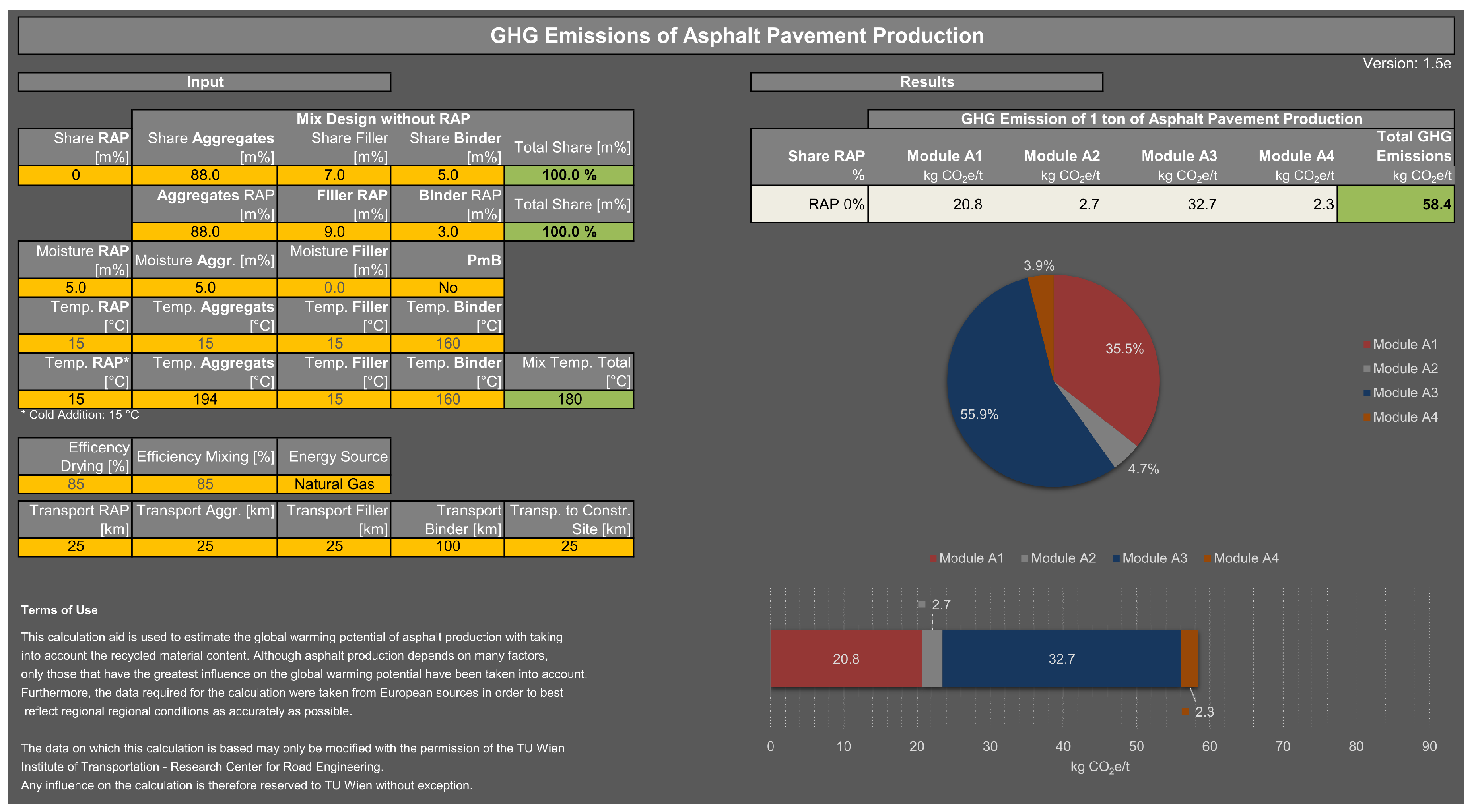
As shown, there are a variety of different mix designs, especially the asphalt binder content, as well as a variety of different scenarios, including the moisture contents of the mineral aggregates and RAP and the transport distance, that lead to different GHG emissions. Therefore, a single study can only represent a certain combination of these characteristics, or preferably the possible effects in the form of variations.

Exactly these problems were decisive in the development of a calculation tool that enables evaluation of asphalt production for producers in terms of GHG emissions. A screenshot of the current version can be seen in Figure 4. As this tool is used by asphalt production companies to assess their energy demand and GHG emissions, as well as to obtain bonus points in the tendering process, only modules A1 to A4 (cradle-to-gate approach and transport to construction site) are included.

The user interface is vertically divided; the left side allow input from the user, while the right side displays the results in numerical form as well as graphically in absolute and relative terms compared to the final product. On the input side, the following characteristics can be chosen:

• Asphalt pavement mix design (final product)
• Share and composition of RAP
• Water content of materials
• Initial (storage) temperature
• Targeted temperature of each material, resulting in asphalt pavement total temperature
• Efficiency settings, allowing for adjustment to the conditions of different asphalt mixing plants
• Energy source used for heating and drying
• Transport distance to the mixing plant and construction site

4. Comparison—Low Traffic Volume vs. High Traffic Volume Road Section

In order to be able to holistically review GHG emissions on a life-cycle level, two road section were investigated:

• A low traffic volume section with 1 million accumulated equivalent single axle loads (ESALs), leading to a construction type for 0.4 to 1.3 million ESALs, classified as LK 1.3 according to current Austrian guidelines and regulations [21].
• A high traffic volume section with 52.5 million ESALs, leading to a construction type for 42 to 82 million ESALs, classified as LK 82 [21].

These construction types can be seen in Figure 5. Both types consist of two unbound base layers on top of the subgrade: a 30 cm unbound lower base layer and 20 cm unbound upper base layer. Above that, the asphalt pavement starts, and is composed of an asphalt base, asphalt binder, and asphalt surface layer. In the case of LK 1.3, an asphalt binder layer is not necessary due to the low traffic volume. For the following calculation, all asphalt layers are the same type of asphalt as introduced before, with GHG emissions of 54.5 kg CO₂e/t (the worst scenario, that is, 5% moisture content and no RAP). For construction, the unbound layers are not further differentiated and are basically mineral aggregates. Accumulation of GHG emissions for unbound layers includes modules A1–A5 and C1–C4, producing 7.46 kg CO₂e/t, whereas for the transport modules, A4 and C2, a 25 km transport distance is assumed, resulting in a large share of 3.76 kg CO₂e/t (out of 7.46) in terms of total GHG emissions.

For the given section types, LK 82 and LK 1.3, calculations were conducted for 1 m² of asphalt pavement, including construction (LK 82: 47.35 kg CO₂e/m², LK 1.3: 29.63 kg CO₂e/m²) and two asphalt surface layer rehabilitations, i.e., removing the existing asphalt surface layer (4 cm) and paving a new layer after 10 years of use (2 × 5.45 kg CO₂e/m²). The results of LK 82 and LK 1.3 coincide with findings in the literature for low traffic and high traffic volume pavements, with 46 kg CO₂e/m² and 27 kg CO₂e/m², respectively [2]. In addition, in order to place these results in relation to traffic, the total GHG emissions for construction and rehabilitation measures (LK 82: 58.25 kg CO₂e/m², LK 1.3: 40.53 kg CO₂e/m²) are then multiplied by the total width of a two-lane road section (2 × 3.5 m, not including road shoulders), leading to 408 kg CO₂e/m of road for LK 82 and 284 kg CO₂e/m of road for LK 1.3, respectively. Detailed information can be found in

Table A7. Construction of 1 m² of road section.

		LK 82	LK 1.3
Type	Unit	1 m²	1 m²
Asphalt Pavement	cm	29	16
Unbound Upper Base	cm	20	20
Unbound Lower Base	cm	30	30
Asphalt Pavement	t	0.73	0.40
Asphalt Pavement	kg CO2e/m²	39.51	21.80
Unbound Base - Aggregates	t	1.05
Asphalt Pavement	kg CO2e/m²	7.83
Total GHG Emissions	kg CO2e/m²	47.35	29.63
Rehabilitation of Surface Layer	t	0.10
Asphalt Pavement	kg CO2e/m²	5.45
Total Constr. & 2 × Rehab.	kg CO2e/m²	58.25	40.53
Two-Lane Road Section (2 × 3.5 m)	kg CO2e/m	408	284

in Appendix A.

In a scenario with 0% moisture in the mineral aggregate instead of 5%, GHG emissions for a road section including two asphalt layer rehabilitations decrease considerably (LK 82: 48.53 kg CO₂e/m², 340 kg CO₂e/m of road (−16.7%); for LK 1.3: 34.23 kg CO₂e/m²), 240 kg CO₂e/m of road (−15.5%)).

To estimate the GHG emissions caused by traffic, an increase of 2% p.a. of traffic is assumed. In addition, the share of electric vehicles (both cars and trucks) is expected to increase by two percentage points (pp) p.a., decreasing fossil fuel-based vehicle use by 2 pp p.a. For an assumed 30-year lifetime of pavement, this scenario is displayed in Appendix A in

Table A9. Traffic for road type LK 82.

	Cars/24h	Trucks/24h	Cars Fossil	Cars Elect.	Trucks Fossil	Trucks Elect.
	+2%p.a.	+2%p.a.	−2 pp p.a.	+2 pp p.a.	−2 pp p.a.	+2 pp p.a.
Year	Vehicles		kg CO2e/Year
2020	27,366	3320	2194	0	1141	0
2021	27,913	3386	2193	10	1440	8
…	…	…	…	…	…	…
2049	47,645	5780	2170	362	1128	299
2050	48,598	5896	2169	379	1128	313
Sum	405.2 Mill.	49.2 Mill.	65,446	5169	34,027	4276
Total	454.4 Mill.		108,918 kg CO2e in 30 years

for LK 82. In summary, the average annual daily traffic (AADT) increases from 30,686 in 2020 (27,366 light vehicles, 3320 heavy vehicles) to 54,494 vehicles (+78%: 48,598 light vehicles, 5896 heavy vehicles) in 2050. If no electric vehicles were used in this 30-year period, the GHG of all fossil-fueled vehicles would accumulate 135,296 kg CO₂e. Due to the assumed increase of electric mobility (pessimistically assuming no further technical improvements in the energy efficacy of electric vehicles will occur), the GHG emissions in this 30-year period amount to 108,918 kg CO₂e (−19% compared to 135,296 kg CO₂e). These figures are based on an assumed consumption of cars (7 L Diesel or 22 kWh electricity per 100 km) and trucks (30 L Diesel or 150 kWh electric energy per 100 km), whereas a 15% excess consumption due to charging losses of electric vehicles is included.

The traffic and GHG emissions analogous to LK 1.3 can be seen in

Table A8. Traffic for road type LK 1.3.

	Cars/24h	Trucks/24h	Cars Fossil	Cars Elect.	Trucks Fossil	Trucks Elect.
	+2%p.a.	+2%p.a.	−2 pp p.a.	+2 pp p.a.	−2 pp p.a.	+2 pp p.a.
Year	Vehicles		kg CO2e/Year
2020	2545	105	204	0	36	0
2021	2596	107	204	1	36	0
…	…	…	…	…	…	…
2049	4431	183	202	34	36	9
2050	4520	186	202	35	36	10
Sum	37.7 Mill.	1.6 Mill.	6086	481	1076	135
Total	39.2 Mill.		7778 kg CO2e in 30 years

in Appendix A. As before, the AADT increases by 2% from 2650 in 2020 (2545 light vehicles, 105 heavy vehicles) to 4706 vehicles (+78%: 4520 light vehicles, 186 heavy vehicles) in 2050. If no electric vehicles were used in this 30-year period, the GHG of all fossil-fueled vehicles would accumulate 9742 kg CO₂e. Due to the assumed increase of electric mobility (+2 pp p.a. pessimistically assuming no further technical improvement of energy-efficacy of electric vehicles will occur), the GHG emissions in this 30-year period amount to 7778 kg CO₂e (−20% compared to 9742 kg CO₂e).

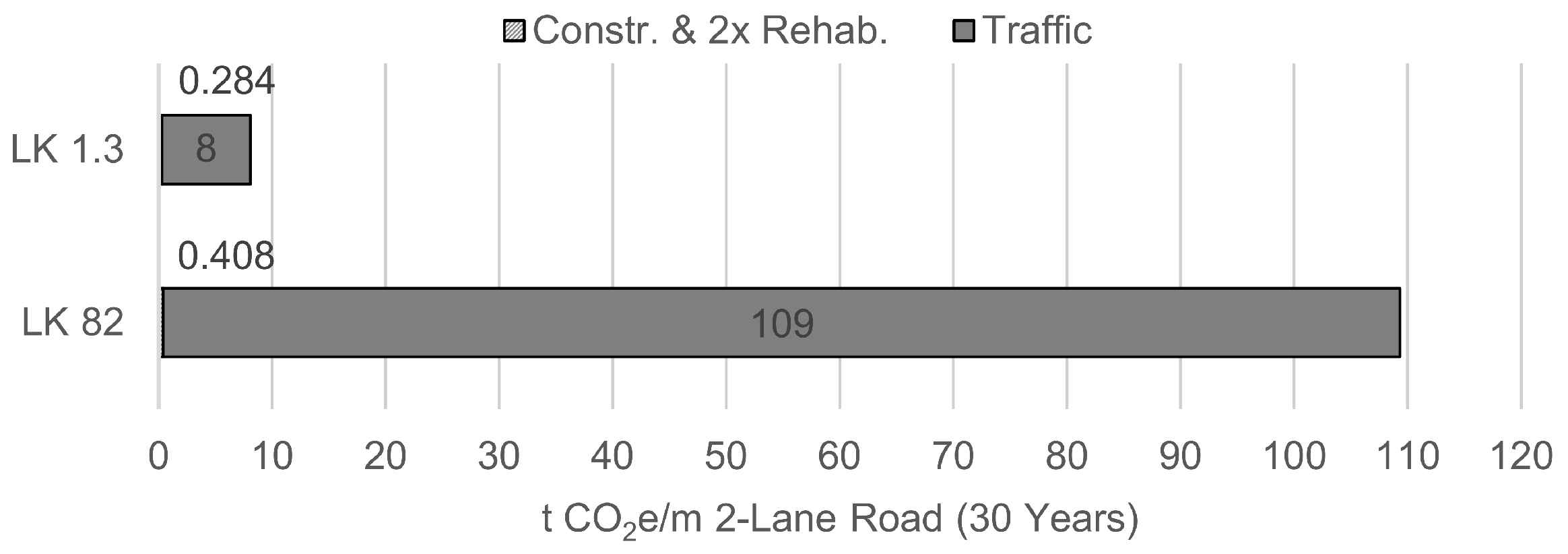
As seen in Figure 6, displaying the GHG emissions for a period of 30 years considering construction of the two-lane road (2 × 3.5 m), rehabilitation, and traffic reveals the enormous share of the latter. In this figure, the construction and rehabilitation category is not visible due to its small proportion, which for LK 82 is 0.408 compared to 109 tons CO₂e and for LK 1.3 is 0.284 compared to 8 tons CO₂e.

5. Conclusions

The aim of this work was to investigate the GHG emissions of asphalt pavement production and the extent of influencing factors during production, as well as to compare GHG emissions for a 30-year lifetime of asphalt pavement in low traffic and high traffic volume road sections (including rehabilitation measures, i.e., complete replacement of the asphalt surface layer every 10 years). In this scenario, ongoing operational measures such as winter maintenance, cleaning, etc., are not considered.

For the first part, the product one ton of asphalt pavement was divided into different stages according to EN 15804: the product stage (including modules A1–A3, representing raw material supply, transport, and manufacturing), construction process stage (modules A4–A5, representing transport and construction), end of life stage (modules C1–C4, representing deconstruction, transport, waste processing, and disposal), and benefits and loads beyond system boundary stage (module D, representing the potential for reuse, recovery, and recycling). For a clear overview, the main results are listed below.

5.1. Production Stage—Modules A1 to A3

• Mix design: 95% mineral aggregates (of which 7 pp are filler) and 5% asphalt binder.
• A1—Raw Material Supply: with average GHG emissions of 2.51 kg CO₂e/t of mineral aggregate and 365 kg CO₂e/t of asphalt binder (note: with high variation of 142 kg CO₂e/t), this module accumulates to 20.6 kg CO₂e/t of asphalt pavement.
• A2—Transport to Manufacturing: transportation of the raw materials to the batch asphalt mixing plant is assumed to involve 25 km from the quarry and 100 km from the asphalt binder supply, and totals 2.2 kg CO₂e/t of asphalt pavement.
• A3—Production: for the above mix design and asphalt pavement temperature of 180 °C, the total GHG emissions are 24.3 kg CO₂e/t when using natural gas as the energy source and accounting for high moisture content of 5% in mineral aggregates (0% moisture: 13.8 kg CO₂e/t). This result includes heating and electrical energy, which contribute as follows:

  –

  Energy demand, and consequently GHG emissions (using natural gas for heating and drying) increase massively, from 0% moisture (47.5 kWh/t, for natural gas: 12.4 kg CO₂e/t) to 5% moisture (88.1 kWh/t, 22.9 kg CO₂e/t).

  –

  The electrical energy required to operate the plant is highly dependent on the production volume, and averages 4 kWh/t (Austrian Energy Mix: 1.4 kg CO₂e/t).

Summarising modules A1 to A3 (cradle-to-gate approach) shows total GHG emissions of 47.1 kg CO₂e/t assuming 5% moisture in natural aggregates (0%: 36.6 kg CO₂e/t).

5.2. Construction Process Stage—Modules A4 to A5

In the construction process stage, a total of 3.3 kg CO₂e/t of GHG emissions are generated, consisting of the following modules:

• A4—Transport: 25 km transportation to the construction site, with 1.9 kg CO₂e/t.
• A5—Construction: paving and compacting on site, generating 1.4 kg CO₂e/t.

5.3. End of Life Stage—Modules C1 to C4

The GHG emissions of the end of life stage amount to 4.1 kg CO₂e/t.

• C1—Deconstruction: milling of asphalt pavement generates 2.09 kg CO₂e/t.
• C2—Transport: a 25 km transport distance to the processing site leads to 1.9 kg CO₂e/t.
• C3—Waste Processing: if hazardously contaminated, which is the case for less than 1% of RAP, landfilling is permitted; emissions are 0 kg CO₂e/t.
• C4—Disposal: on average, 12% of RAP is landfilled, which results in less than 0.1 kg CO₂e/t being generated.

Under these assumptions, the total GHG emissions of one ton of asphalt pavement, including all modules A1–A5 and C1–C4 and without including B1–B7 or D from the use stage, amount to 54.5 kg CO₂e/t with 5% moisture content in the mineral aggregate, and to 44.0 kg CO₂e/t with 0% moisture.

5.4. Variation of the Asphalt Binder Footprint and Mineral Aggregates

Although the asphalt binder typically accounts for about 5% of the mass of asphalt pavement and its footprint (module A1) and deviation are very high at 365 ± 142 kg CO₂e/t (or ±39%), the variation of the footprint accounts for “only” a 13% change in total GHG emissions (54.5 ± 7.1 kg CO₂e/t). In contrast, the mineral aggregates have a small footprint (2.51 ± 0.49 kg CO₂e/t) and a high share of around 95% by mass, affecting only 1% of total GHG emissions (54.5 ± 0.5 kg CO₂e/t).

5.5. Benefits and Loads beyond System Boundary

Finally, module D considers the loads and benefits of RAP by reducing the need for virgin materials. Assuming the addition of 300 kg of RAP (=30% recycling rate), consisting of 97% mineral aggregates (of which are 9 pp filler) and 3% asphalt binder, the GHG emissions to be reduced in module D recycling potential amount to −3.9 kg CO₂e/t asphalt pavement (with 30% RAP). Different shares of RAP show a reduction of 1.3 and 6.5 kg CO₂e/t asphalt pavement for 10% and 50% RAP, respectively.

These results are only valid for the assumed aspects; other scenarios may have different effects on GHG emissions. Therefore, a calculation tool was developed for asphalt production companies to asses their influence on climate change, as well as to be able to earn bonus points in the tendering process for high level network roads if certain emission limits are undershot.

5.6. Comparing Pavement Production (Including Rehabilitation) to Traffic

Furthermore, a portion of the use stage for a period of 30 years was calculated seperately for a high traffic road and a low traffic volume road, including rehabilitation measures (i.e., completely replacing the asphalt surface layer every 10 years). Because only parts of the use stage with modules B1 to B7 are considered (ongoing operational measures such as winter maintenance, cleaning, etc., are not considered), the results are not directly linked to the corresponding stage. Instead, they are presented to help estimate and contrast the orders of magnitude of the production of a two-lane asphalt road (7 m width) and the traffic passing over it.

• A high traffic volume two-lane road (AADT 30,000 with an 2% p.a. increase to 54,000 vehicles in 30 years) accumulates 135 t CO₂e per metre. If an increasing share of electric vehicles over 30 years is additionally assumed, this figure changes to 109 t CO₂e per metre.
• A low traffic volume two-lane road (AADT increase from 2600 to 4700 in 30 years) accumulates GHG emissions of 9.8 t CO₂e per metre in 30 years, or 8 t CO₂e/m with increasing share of electric vehicles.
• In this context, the GHG emissions due to the construction and rehabilitation processes are vanishingly small, with a total of 0.284 t CO₂e per metre of two-lane road for a low traffic volume road (LK 1.3) and 0.408 t CO₂e per metre of two-lane road for a high traffic volume road (LK 82).

In conclusion, this study illustrates the benefits of a structured presentation of the results in order to create comparability and thereby fulfil the objective of EN 15804. As a next step, the theoretical approaches for calculating the energy consumption of drying and heating the material need to be verified or adapted using results from practice. Even though the production process results in relatively low GHG emissions compared to traffic, it nonetheless remains of the utmost importance to reduce those emissions that are within the sphere of the construction industry in order to meet climate goals.