
Wind Effects on Dome Structures and Evaluation of CFD Simulations through Wind Tunnel Testing

Abstract
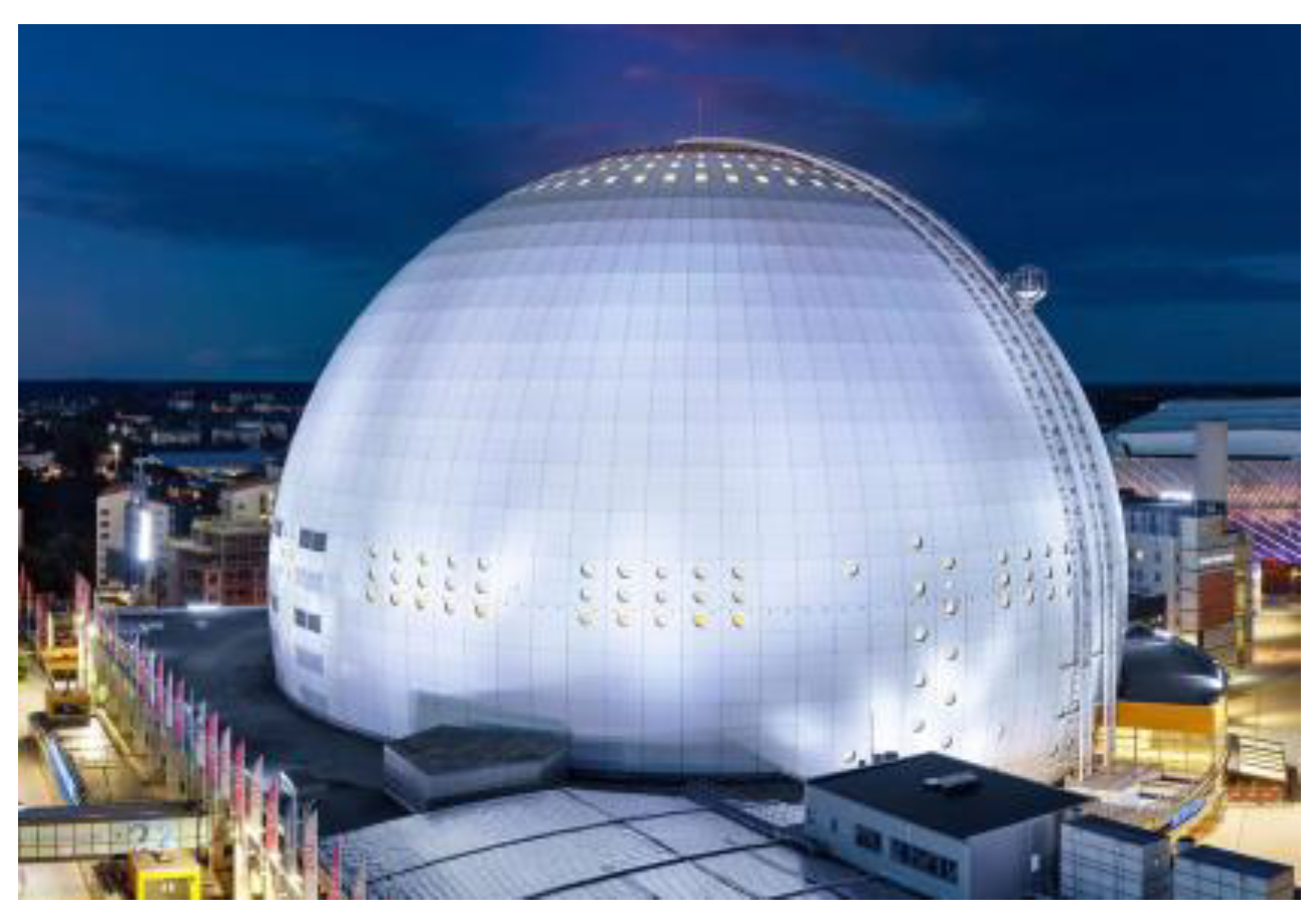
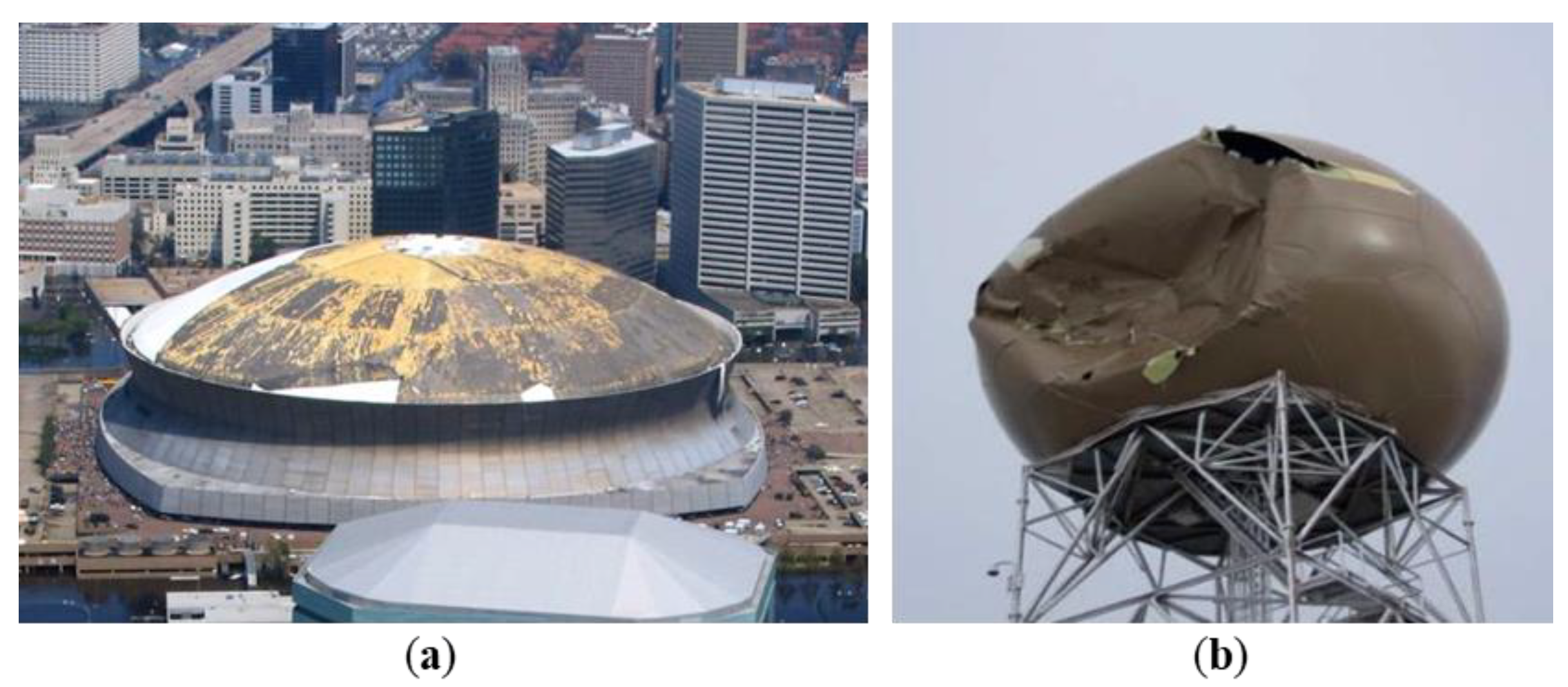
:1. Introduction
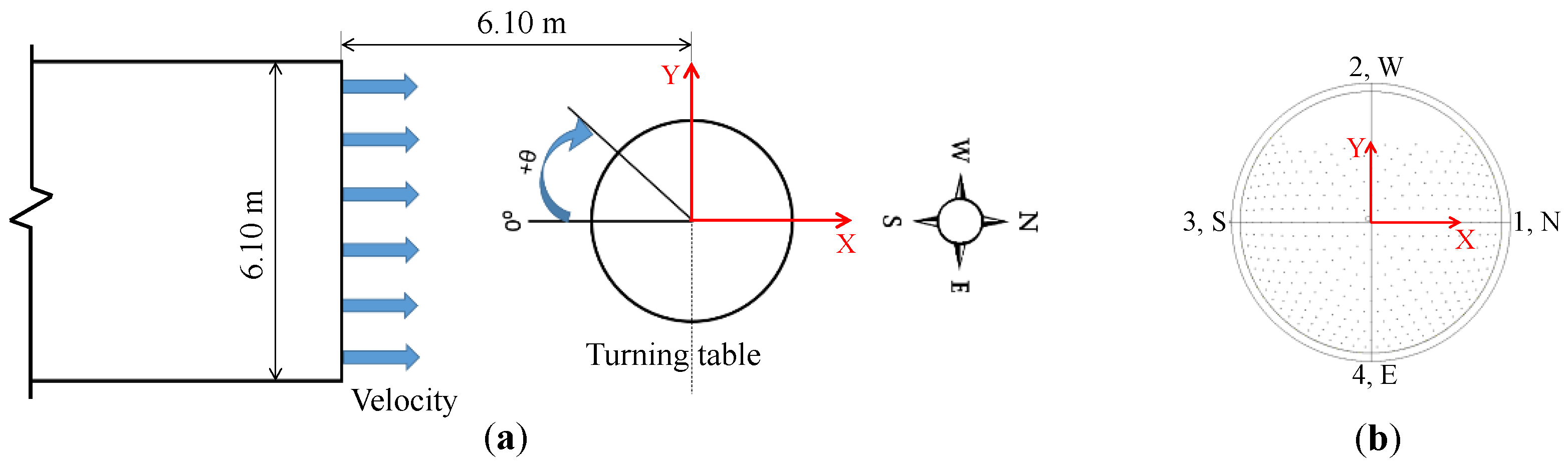
2. Experimental Setup
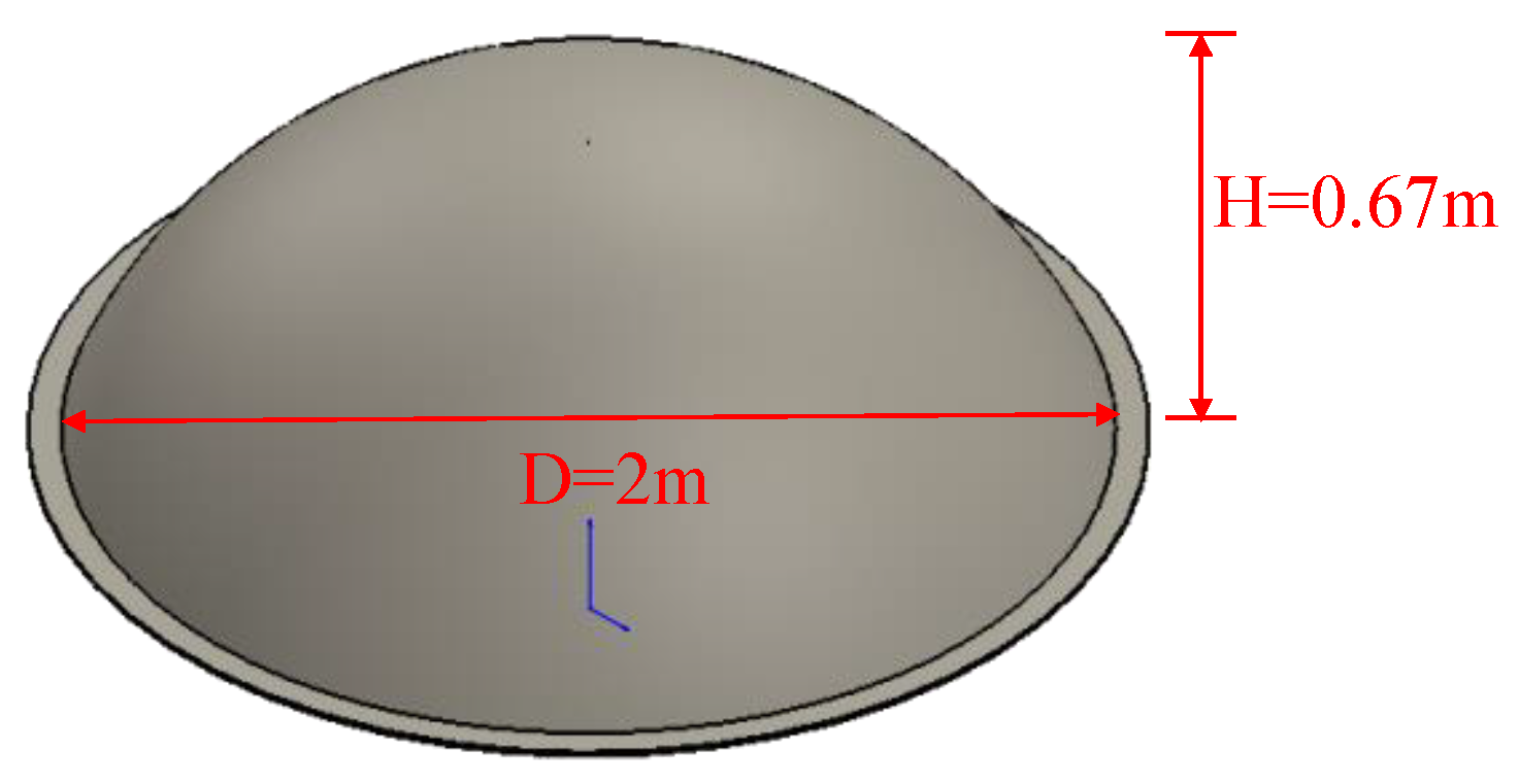
2.1. Dome Geometry
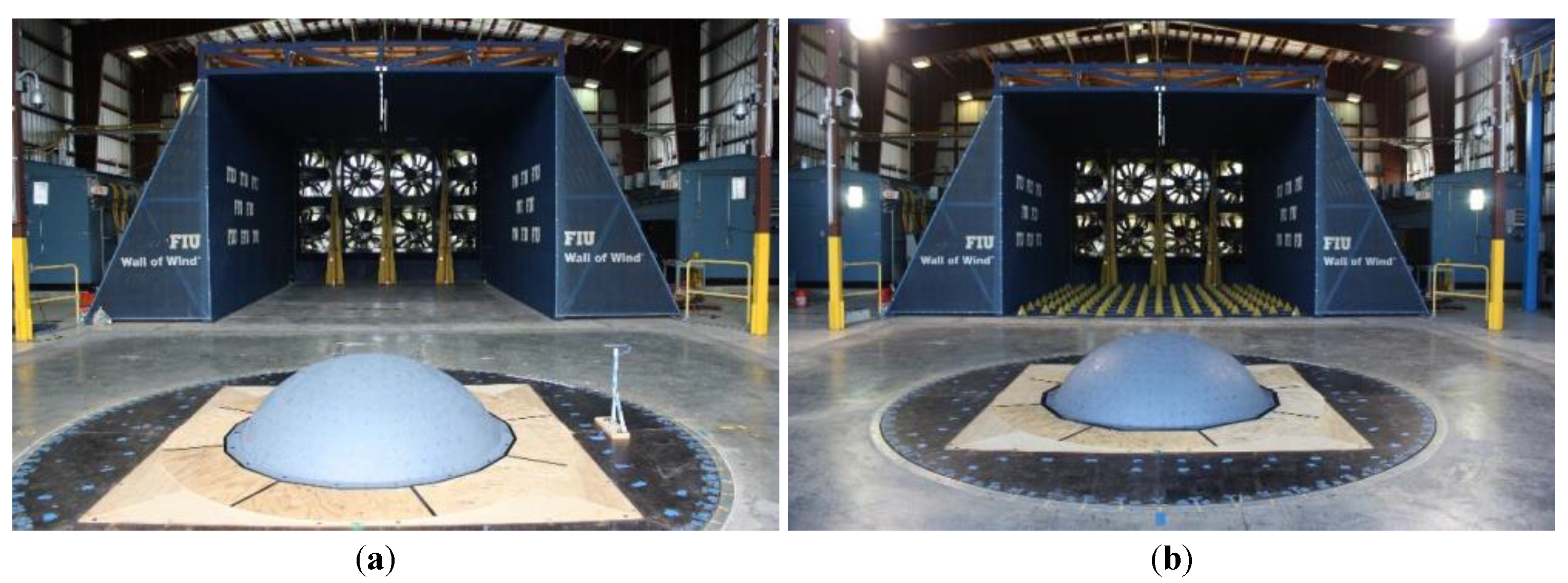
2.2. Introduction of WOW EF
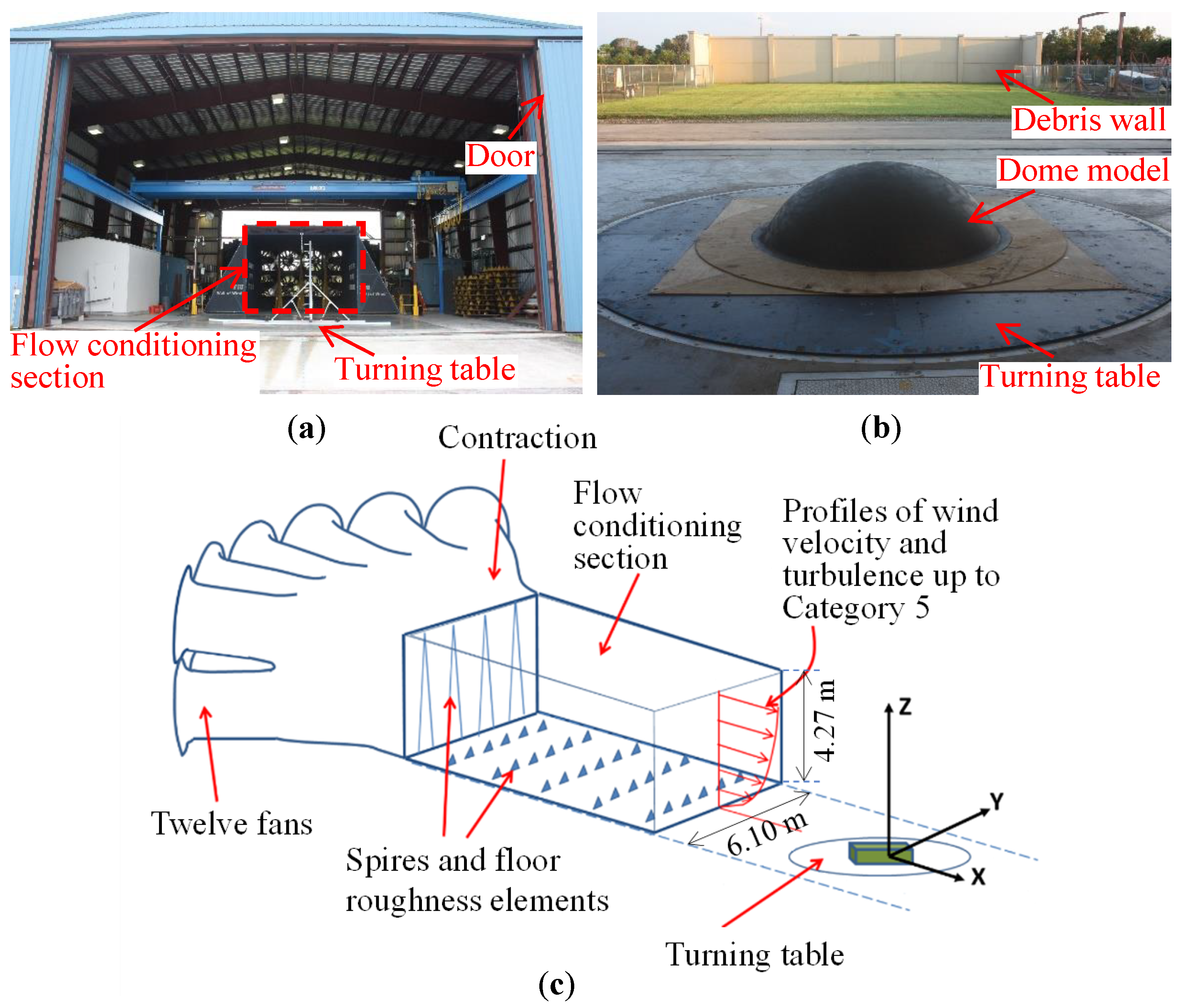
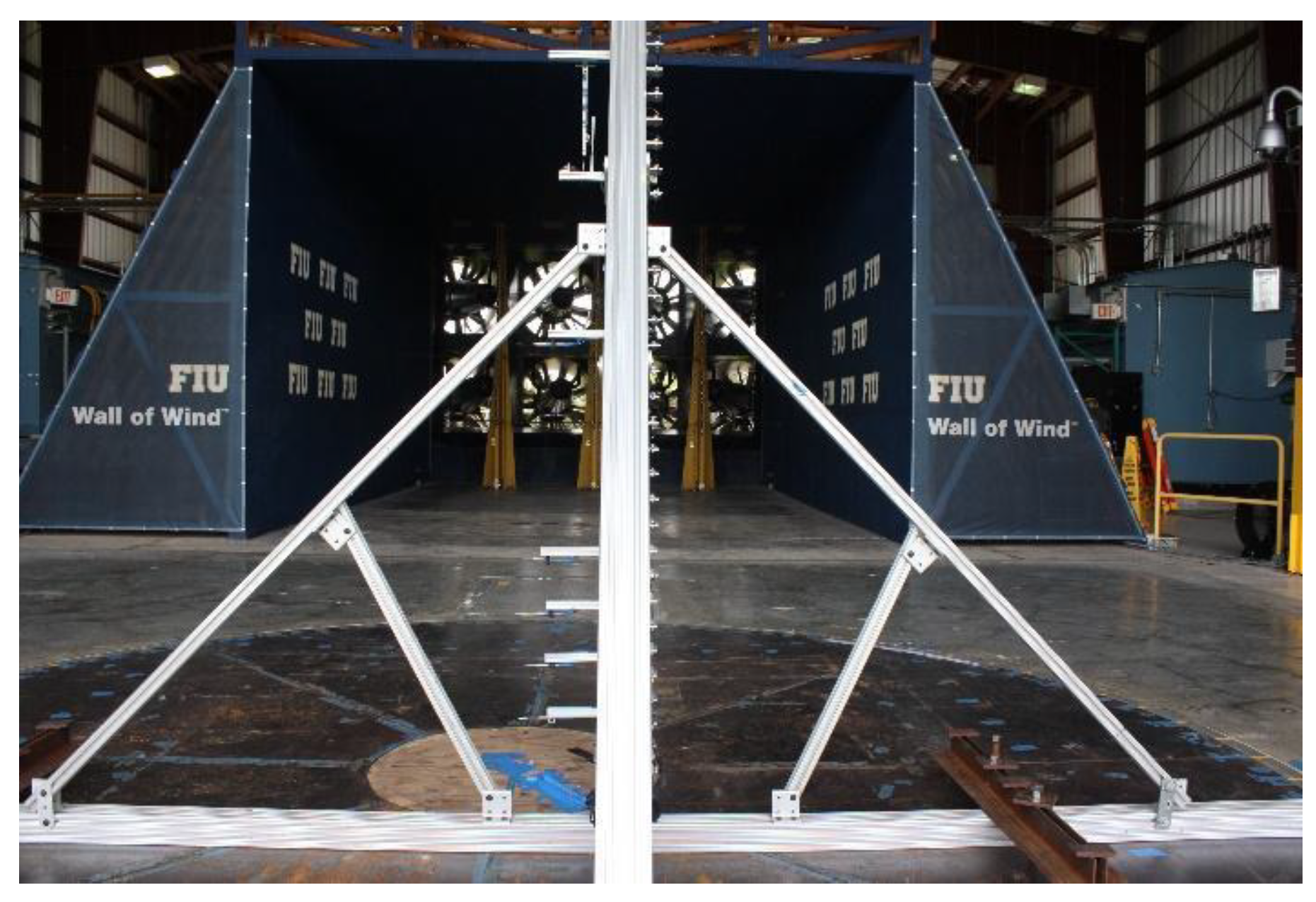
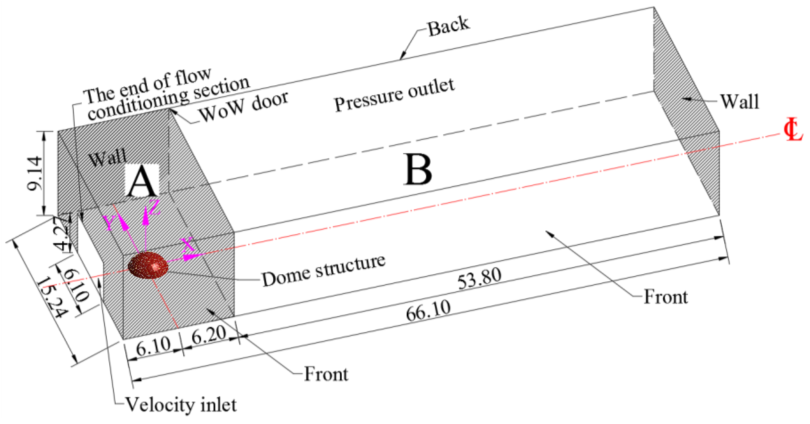
2.3. Experimental Setup
2.4. Testing Cases
3. Experimental Results and Discussion
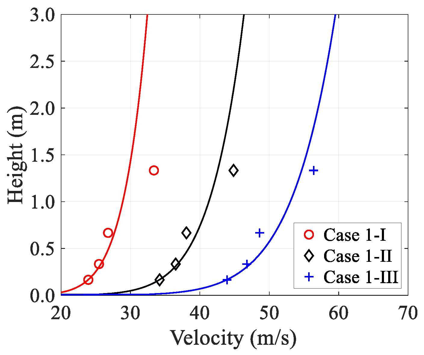
3.1. Mean Velocity Profile
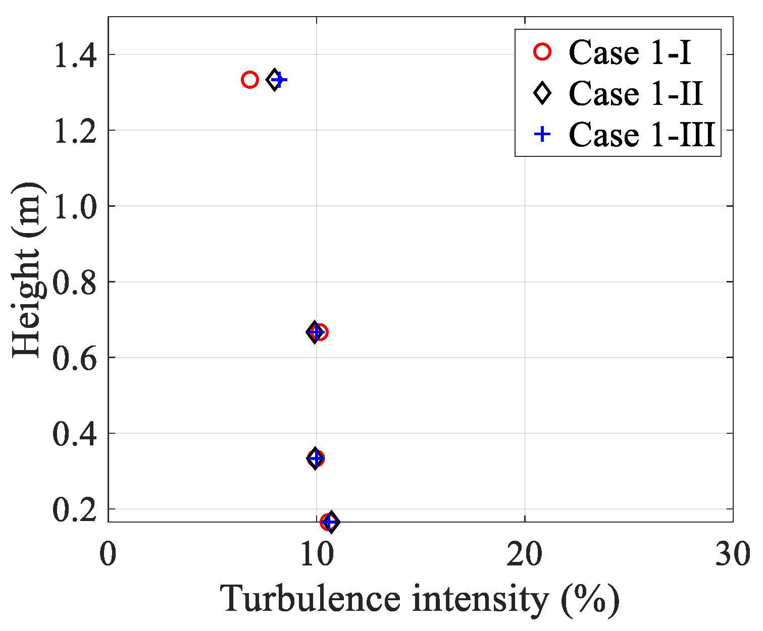
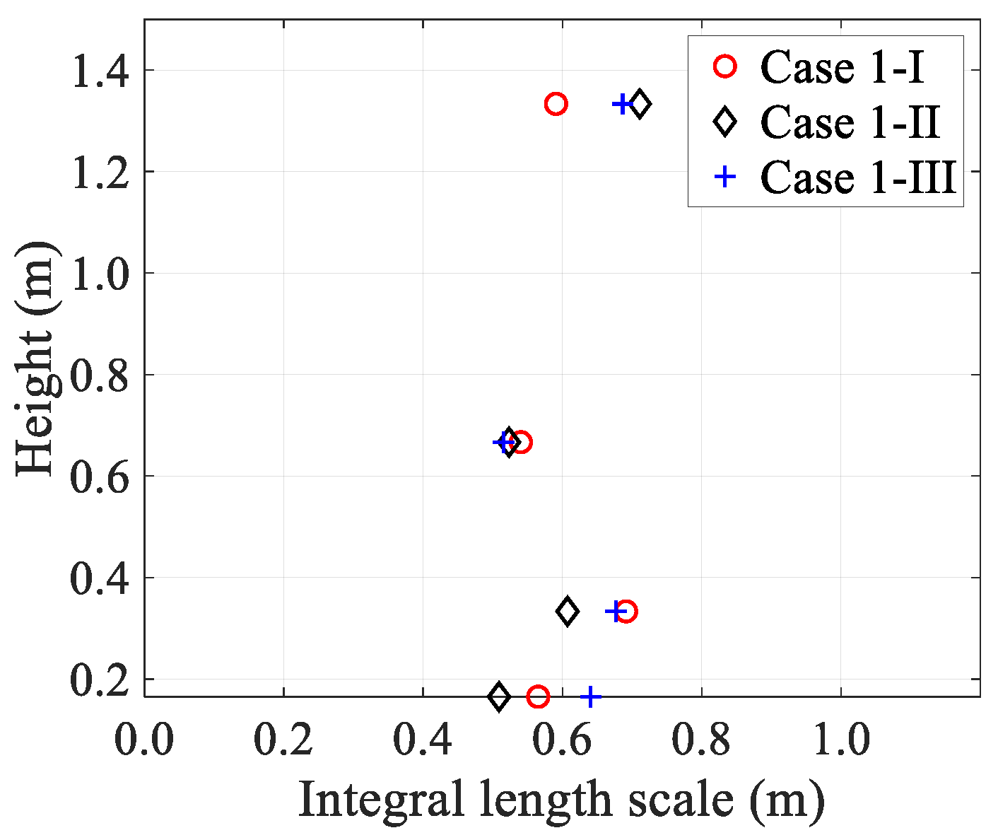
3.2. Turbulence Intensity and Integral Length Scale
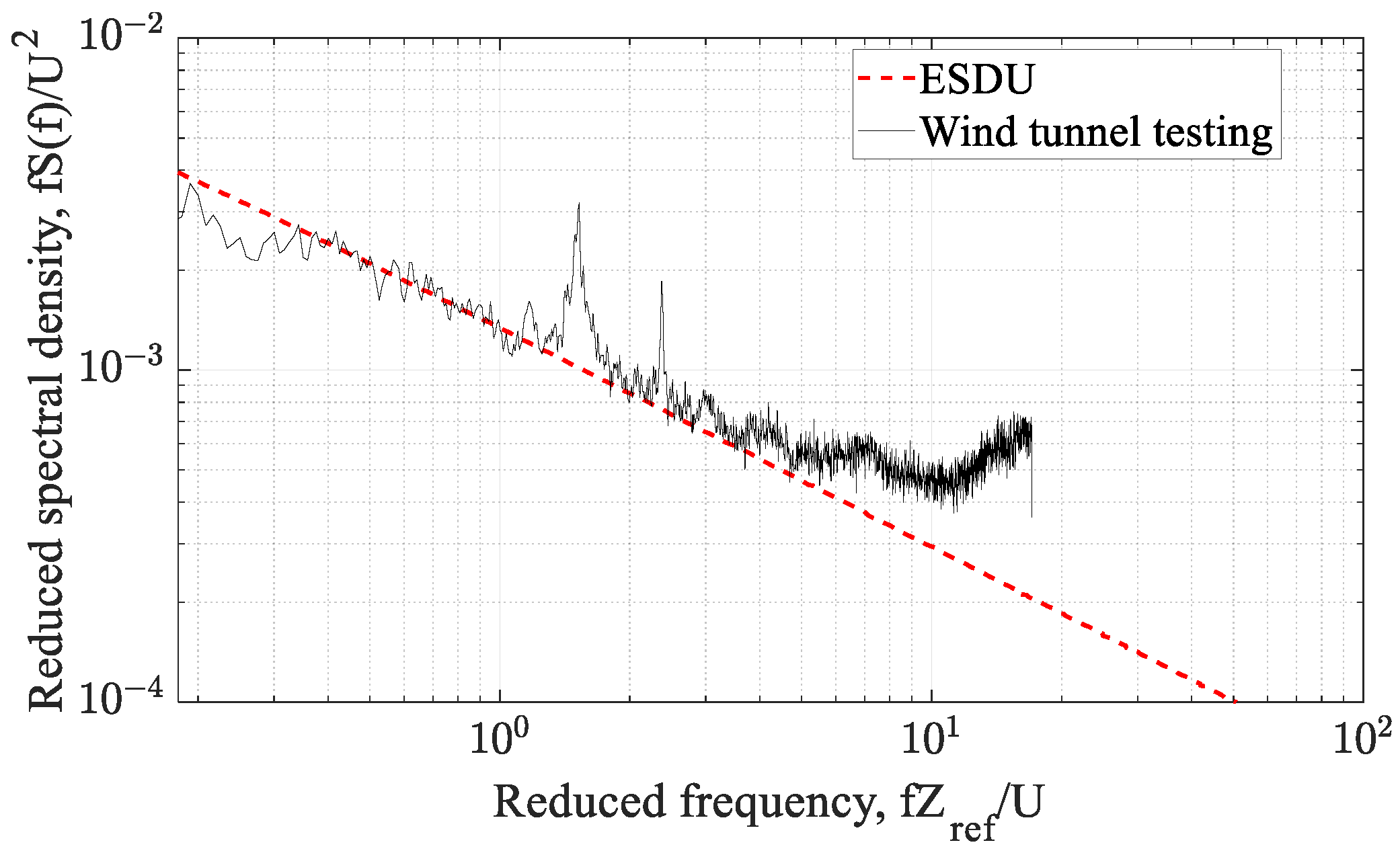
3.3. Power Spectral Density
3.4. Reynolds Number
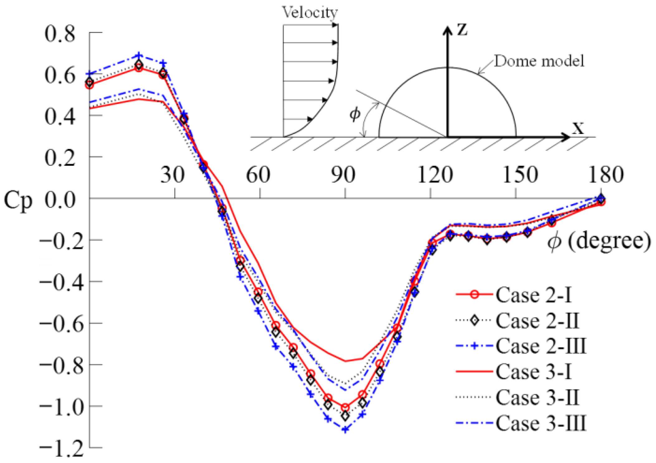
3.5. Mean Pressure Coefficient on the Center Meridian of the Model
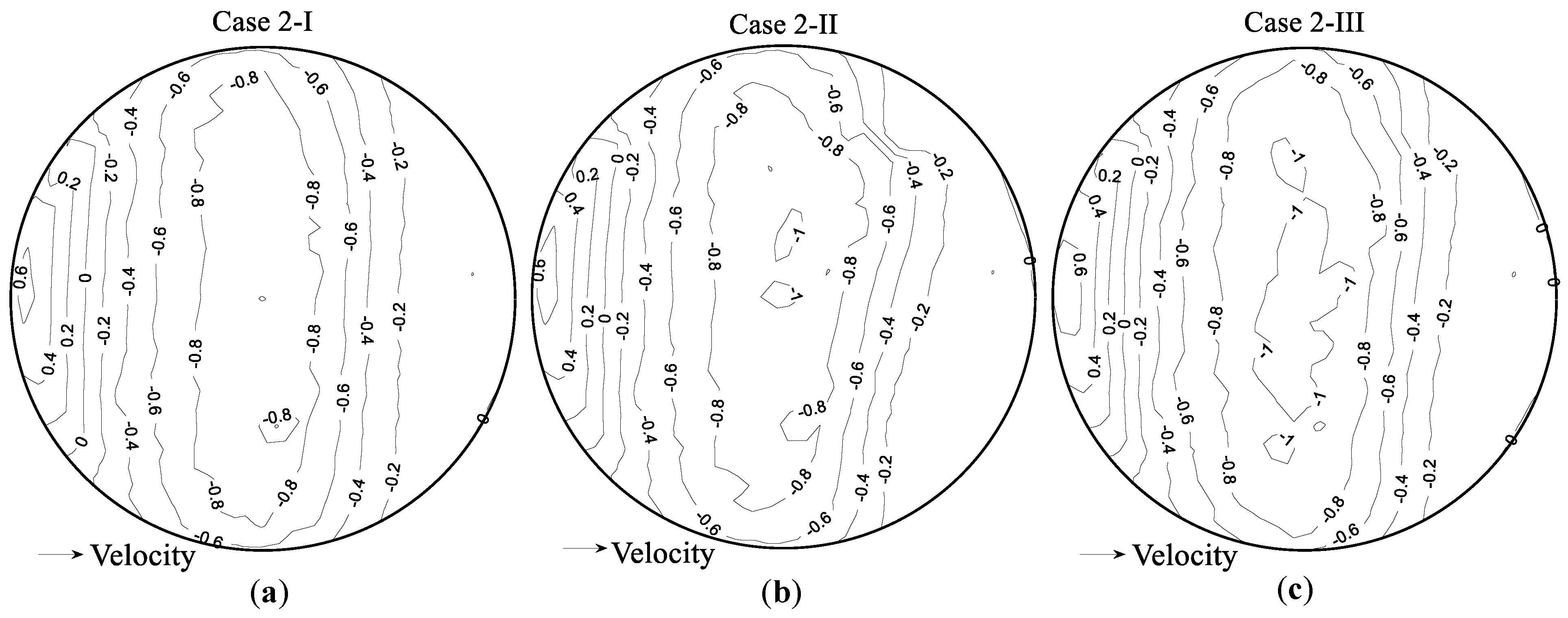
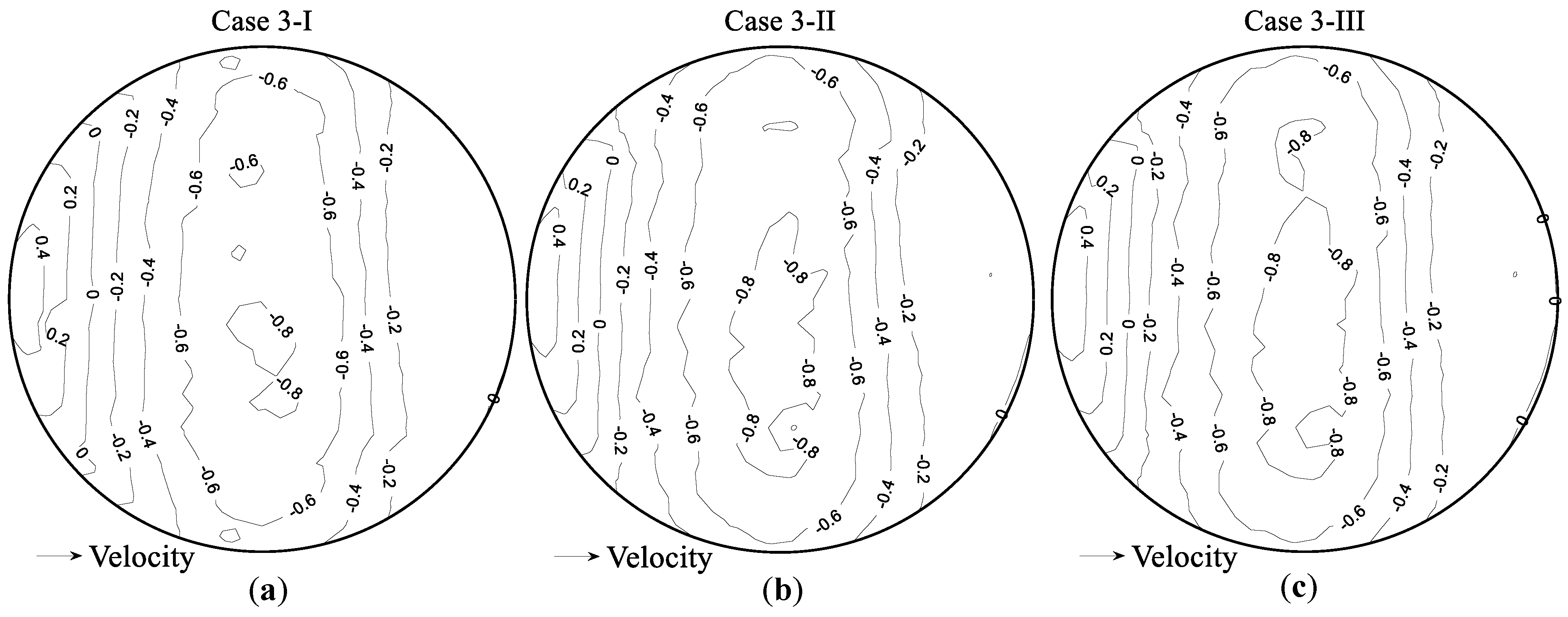
3.6. Wind Pressure Distribution on Dome Surface
3.6.1. Open Terrain
3.6.2. Suburban Terrain
3.7. Force and Moment Coefficient
4. Numerical Simulations and Discussion of Results
4.1. Numerical Simulations of Wind Tunnel Testing
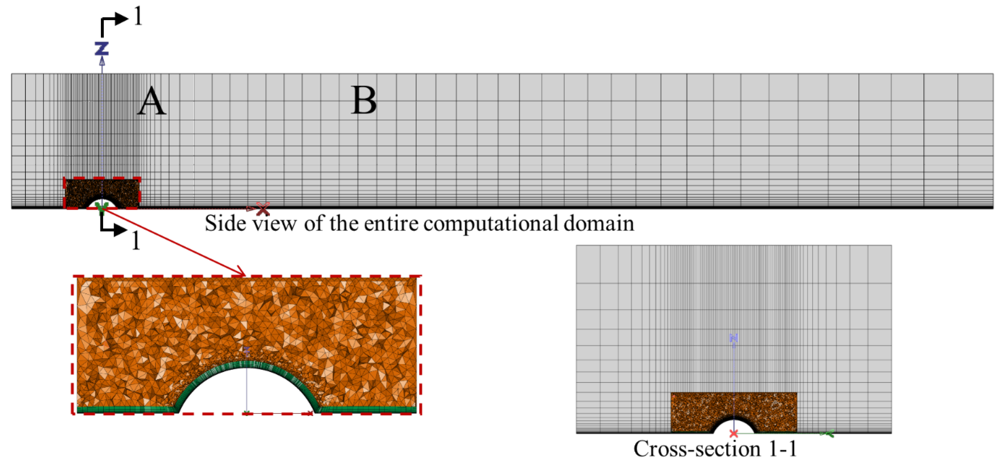
4.1.1. Numerical Model
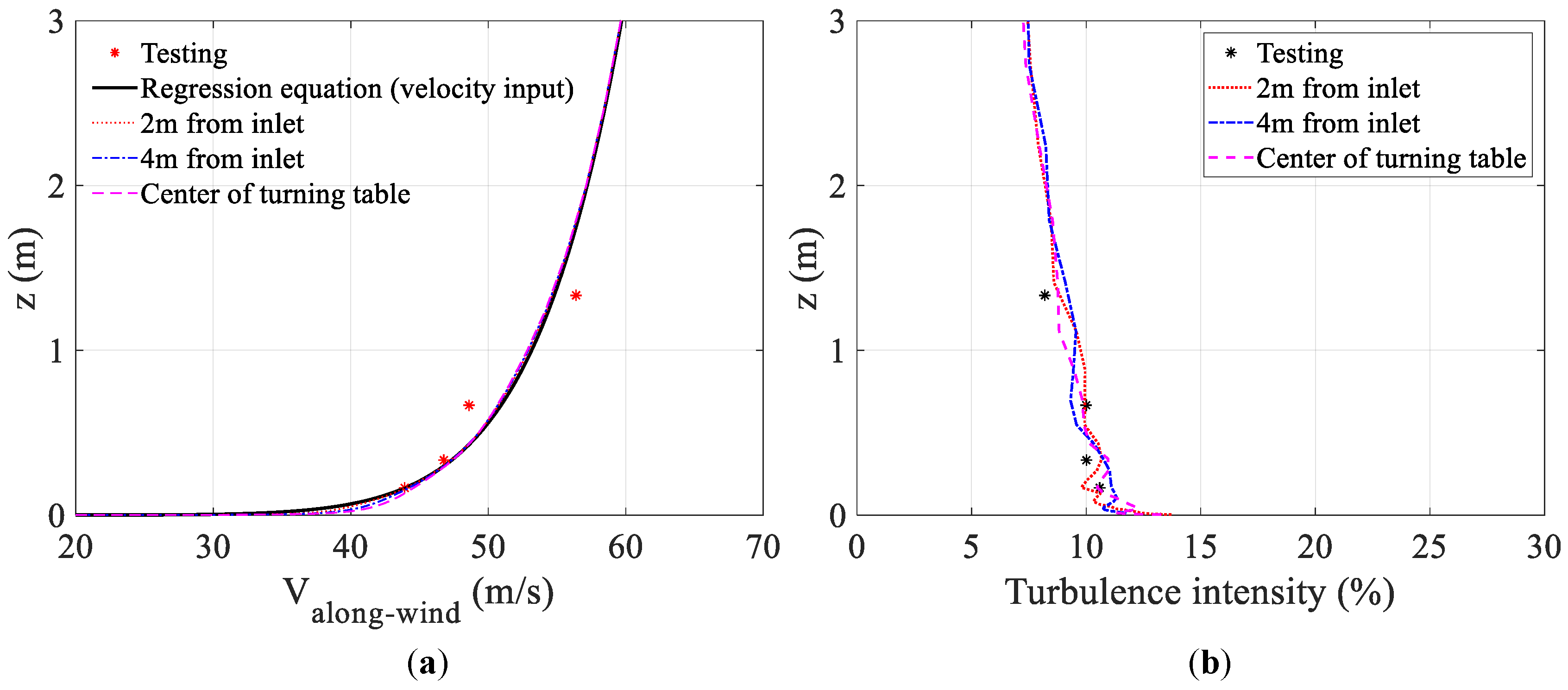
4.1.2. Determination of Velocity Input
4.1.3. CFD Simulation Setup
4.2. Discussion of Results
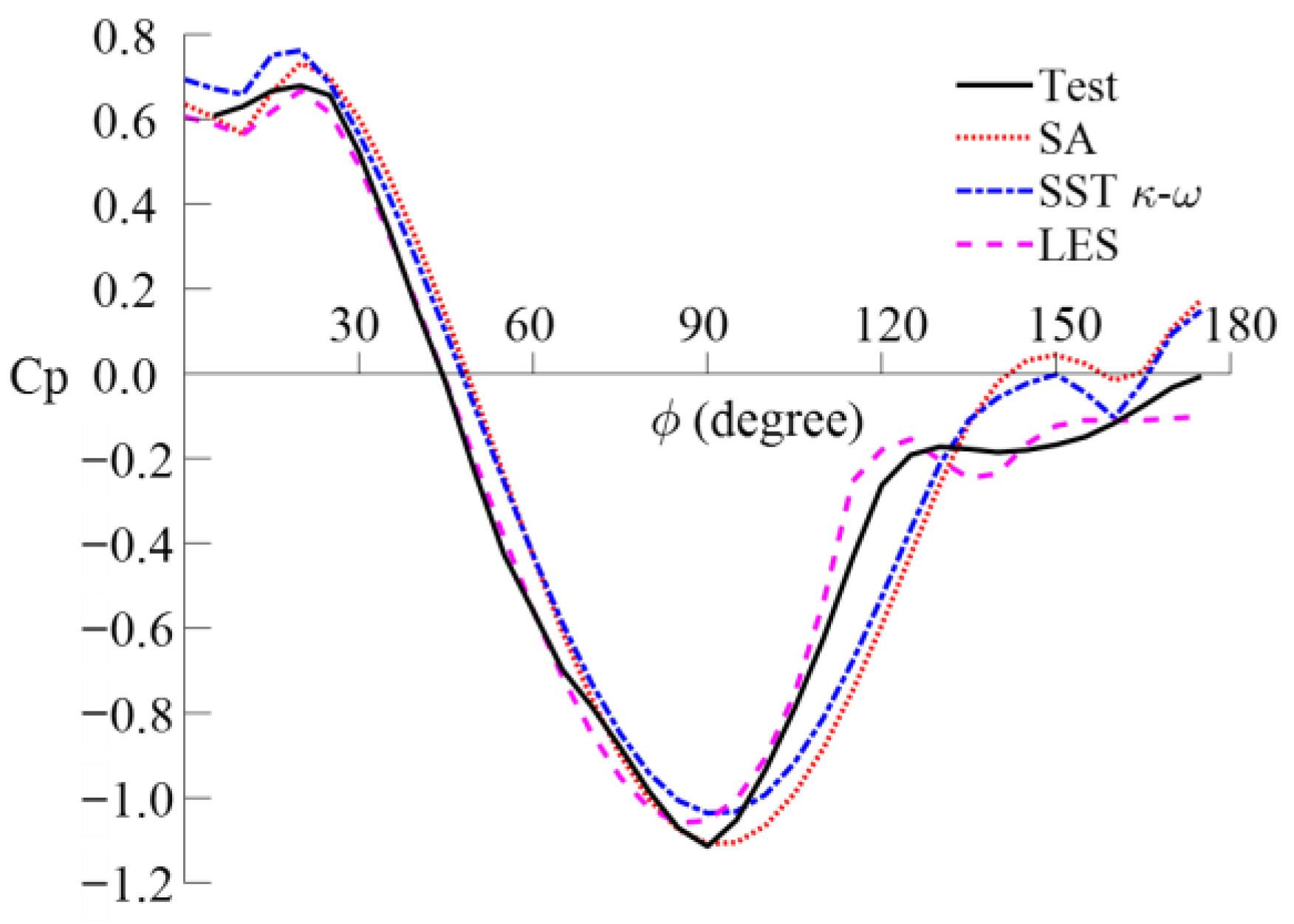
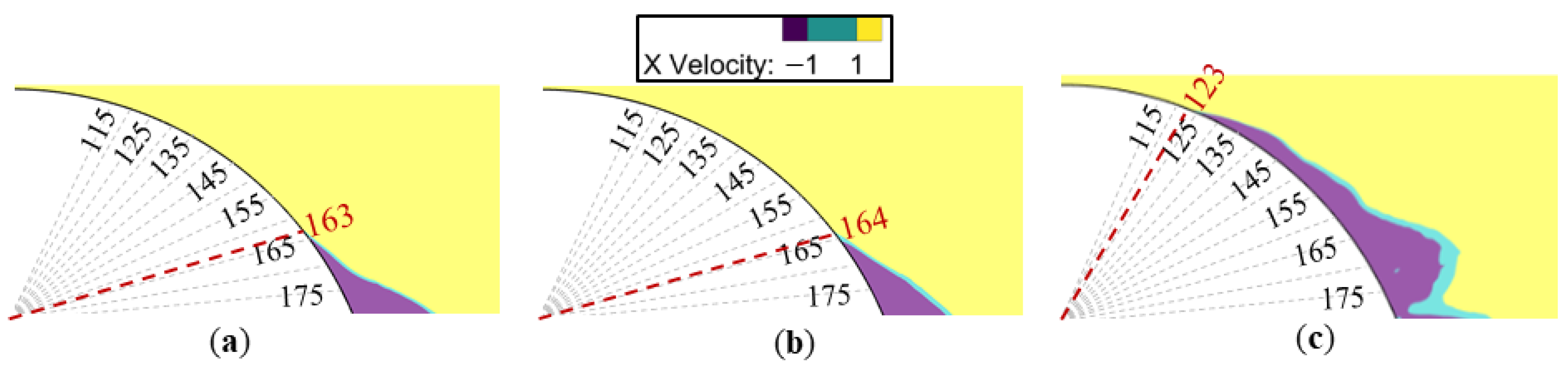
4.2.1. Mean Pressure Coefficient
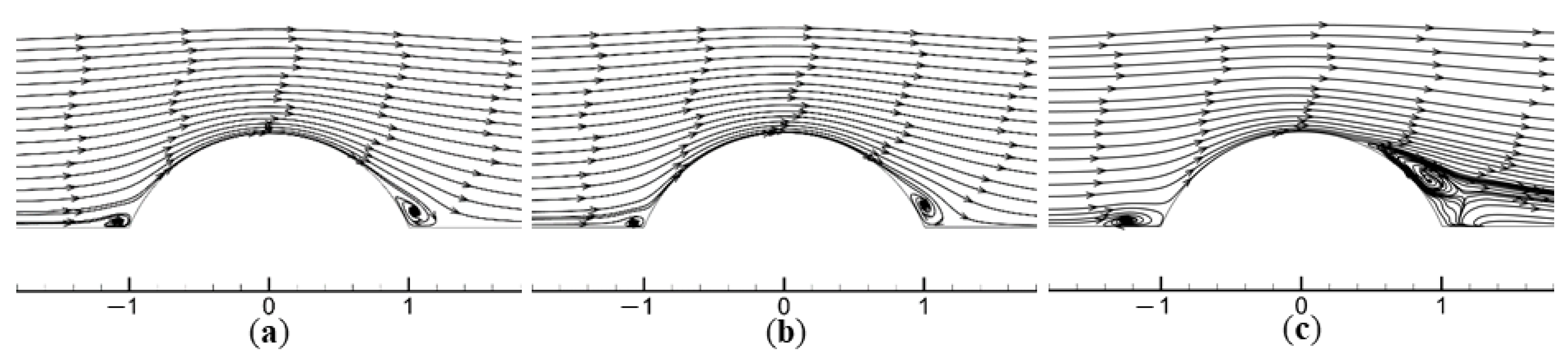
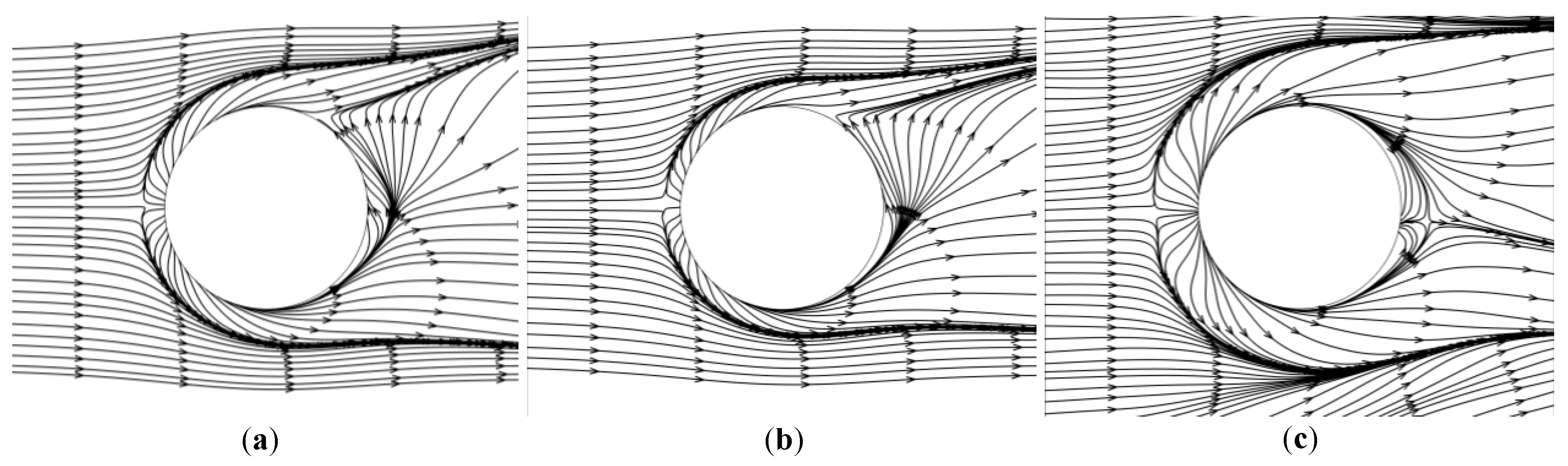
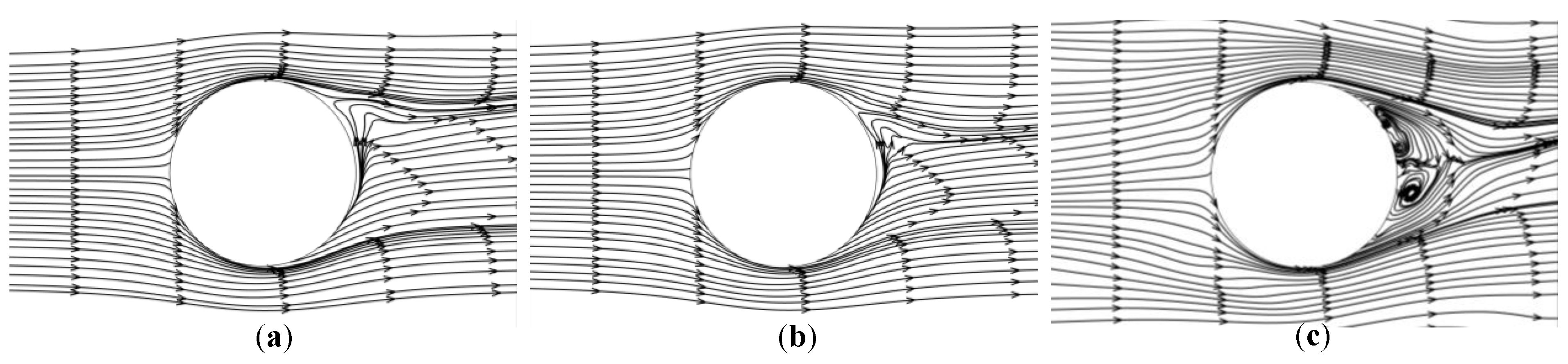
4.2.2. Time Averaged Streamlines
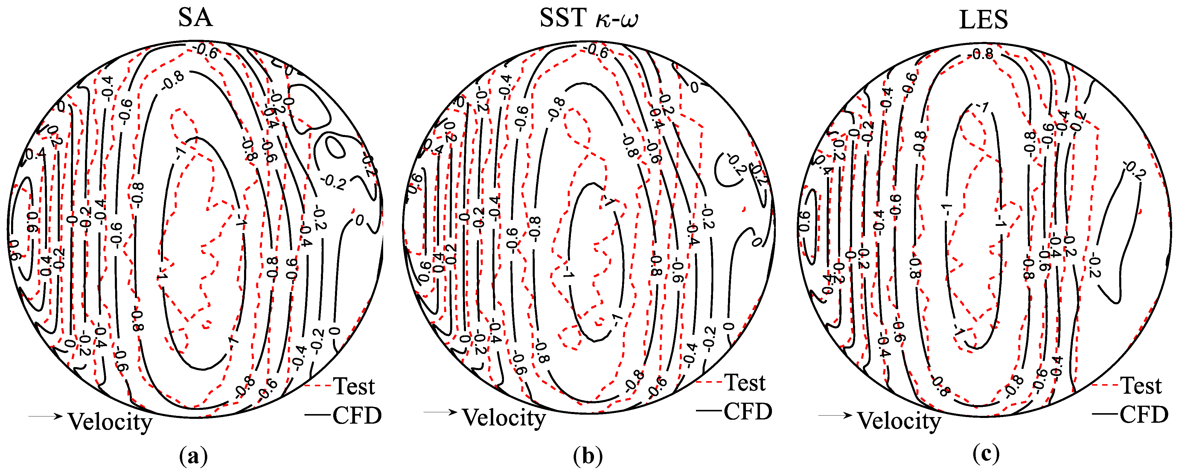
4.2.3. Instantaneous Turbulence Structure
5. Conclusions
Author Contributions
Funding
Institutional Review Board Statement
Informed Consent Statement
Data Availability Statement
Acknowledgments
Conflicts of Interest
References
- Maher, F.J. Wind loads on basic dome shapes. J. Struct. Div. 1965, 91, 219–228. [Google Scholar] [CrossRef]
- Taniguchi, S.; Sakamoto, H.; Kiya, M.; Arie, M. Time-averaged aerodynamic forces acting on a hemisphere immersed in a turbulent boundary. J. Wind Eng. Ind. Aerod. 1982, 9, 257–273. [Google Scholar] [CrossRef]
- Taylor, T.J. Wind pressures on a hemispherical dome. J. Wind Eng. Ind. Aerod. 1992, 40, 199–213. [Google Scholar] [CrossRef]
- Ogawa, T.; Nakayama, M.; Murayama, S.; Sasaki, Y. Characteristics of wind pressures on basic structures with curved surfaces and their response in turbulent flow. J. Wind Eng. Ind. Aerod. 1991, 38, 427–438. [Google Scholar] [CrossRef]
- Savory, E.; Toy, N. Hemisphere and hemisphere-cylinders in turbulent boundary layers. J. Wind Eng. Ind. Aerod. 1986, 23, 345–364. [Google Scholar] [CrossRef]
- Letchford, C.W.; Sarkar, P.P. Mean and fluctuating wind loads on rough and smooth parabolic domes. J. Wind Eng. Ind. Aerod. 2000, 88, 101–117. [Google Scholar] [CrossRef]
- Cheng, C.M.; Fu, C.L. Characteristic of wind loads on a hemispherical dome in smooth flow and turbulent boundary layer flow. J. Wind Eng. Ind. Aerod. 2010, 98, 328–344. [Google Scholar] [CrossRef]
- Chevula, S.; Sanz-Andres, A.; Franchini, S. Aerodynamic external pressure loads on a semi-circular bluff body under wind gusts. J. Fluid Struct. 2015, 54, 947–957. [Google Scholar] [CrossRef]
- Kim, Y.C.; Yoon, S.W.; Cheon, D.J.; Song, J.Y. Characteristics of wind pressures on retractable dome roofs and external peak pressure coefficients for cladding design. J. Wind Eng. Ind. Aerod. 2019, 188, 294–307. [Google Scholar] [CrossRef]
- Lee, J.H.; Kim, Y.C.; Cheon, D.J.; Yoon, S.W. Wind pressure characteristics of elliptical retractable dome roofs. J. Asian Archit. Build. 2022, 21, 1561–1577. [Google Scholar] [CrossRef]
- Tavakol, M.M.; Yaghoubi, M.; Ahmadi, G. Experimental and numerical analysis of airflow around a building model with an array of domes. J. Build. Eng. 2021, 34, 101901. [Google Scholar] [CrossRef]
- Murakami, S. Overview of turbulence models applied in CWE–1997. J. Wind Eng. Ind. Aerod. 1998, 74–76, 1–24. [Google Scholar] [CrossRef]
- Smagorinsky, J. General circulation experiments with the primitive equations: I. The basic experiment. Mon. Weather Rev. 1963, 91, 99–164. [Google Scholar] [CrossRef]
- Nicoud, F.; Ducros, F. Subgrid-scale stress modelling based on the square of the velocity gradient tensor. Flow Turbul. Combust. 1999, 62, 183–200. [Google Scholar] [CrossRef]
- Germano, M.; Piomelli, U.; Moin, P.; Cabot, W.H. A dynamic subgrid-scale eddy viscosity model. Phys. Fluids A-Fluid 1991, 3, 1760. [Google Scholar] [CrossRef] [Green Version]
- Lilly, D.K. A proposed modification of the Germano subgrid-scale closure method. Phys. Fluids A-Fluid 1992, 4, 633–635. [Google Scholar] [CrossRef]
- Spalart, P.; Allmaras, S. A one-equation turbulence model for aerodynamic flows. Rech. Aerospatiale 1994, 1, 5–21. [Google Scholar] [CrossRef]
- Launder, B.E.; Spalding, D.B. Lectures in Mathematical Models of Turbulence; Academic Press: London, UK, 1972. [Google Scholar]
- Wilcox, D.C. Turbulence Modeling for CFD; DCW Industries: La Canada Flintridge, CA, USA, 1998. [Google Scholar]
- Shih, T.H.; Liou, W.W.; Shabbir, A.; Yang, Z.; Zhu, J. A new k-ϵ eddy viscosity model for high reynolds number turbulent flows. Comput. Fluids 1995, 24, 227–338. [Google Scholar] [CrossRef]
- Yakhot, V.S.; Orszag, S.A.; Thangam, S.; Gatski, T.B.; Speziale, C.G. Development of turbulence models for shear flows by a double expansion technique. Phys. Fluids A-Fluid 1992, 4, 1510. [Google Scholar] [CrossRef] [Green Version]
- Menter, F.R. Two-equation eddy-viscosity turbulence models for engineering applications. AIAA J. 1994, 32, 1598–1605. [Google Scholar] [CrossRef] [Green Version]
- Menter, F.R. Eddy viscosity transport equations and their relation to the k-ε model. J. Fluid Eng. 1997, 119, 876–884. [Google Scholar] [CrossRef]
- Menter, F.R.; Kuntz, M.; Langtry, R. Ten years of industrial experience with the SST turbulence model. Turbul. Heat Mass Transf. 2003, 4, 625–632. [Google Scholar]
- Tavakol, M.M.; Yaghoubi, M.; Motlagh, M.M. Air flow aerodynamic on a wall-mounted hemisphere for various turbulent boundary layers. Exp. Therm. Fluid Sci. 2010, 34, 538–553. [Google Scholar] [CrossRef]
- Tavakol, M.M.; Abouali, O.; Yaghoubi, M. Large eddy simulation of turbulent flow around a wall mounted hemisphere. Appl. Math Model 2015, 39, 3596–3618. [Google Scholar] [CrossRef]
- Fu, C.L.; Cheng, C.M.; Lo, Y.L.; Cheng, D.Q. LES simulation of hemispherical dome’s aerodynamic characteristics in smooth and turbulence boundary layer flows. J. Wind Eng. Ind. Aerod. 2015, 144, 53–61. [Google Scholar] [CrossRef]
- Wood, J.N.; De Nayer, G.; Schmidt, S.; Breuer, M. Experimental investigation and large-eddy simulation of the turbulent flow past a smooth and rigid hemisphere. Flow Turbul. Combust. 2016, 97, 79–119. [Google Scholar] [CrossRef] [Green Version]
- Sadeghi, H.; Heristchian, M.; Aziminejad, A.; Nooshin, H. Wind effect on grooved and scallop domes. Eng. Struct. 2017, 148, 436–450. [Google Scholar] [CrossRef]
- Fouad, N.S.; Mahmoud, G.H.; Nasr, N.E. Comparative study of international codes wind loads and CFD results for low rise buildings. Alex. Eng. J. 2018, 57, 3623–3639. [Google Scholar] [CrossRef]
- Khosrowjerdi, S.; Sarkardeh, H.; Kioumarsi, M. Effect of wind load on different heritage dome buildings. Eur. Phys. J. Plus 2021, 136, 1180. [Google Scholar] [CrossRef]
- Franke, J.; Hirsch, C.; Jensen, A.G.; Krüs, H.W.; Schatzmann, M.; Westbury, P.S.; Miles, S.D.; Wisse, J.A.; Wright, N.G. Recommendations on the use of CFD in predicting pedestrian wind environment. In COST Action C14 “Impact of Wind and Storms on City Life and Built Environment”; Von Karman Institute: Rhode-Saint-Genese, Belgium, 2004. [Google Scholar]
- Murakami, S. Setting the scene: CFD and symposium overview. Wind Struct. 2002, 5, 83–88. [Google Scholar] [CrossRef]
- Tominaga, Y.; Stathopoulos, T. Numerical simulation of dispersion around an isolated cubic building: Model evaluation of RANS and LES. Build. Environ. 2010, 45, 2231–2239. [Google Scholar] [CrossRef] [Green Version]
- American Society of Civil Engineers. Minimum Design Loads and Associated Criteria for Buildings and Other Structures; ASCE/SEI 7–16; American Society of Civil Engineers: Reston, VA, USA, 2016. [Google Scholar] [CrossRef]
- Simiu, E.; Scanlan, R.H. Wind Effects on Structures: Fundamentals and Applications to Design, 3rd ed.; John Wiley and Sons, Inc.: New York, NY, USA, 1986. [Google Scholar]
- Kaimal, J.C.; Finigan, J.J. Atmospheric Boundary Layer Flows: Their Structure and Measurement; Oxford University Press: Oxford, UK, 1994. [Google Scholar]
- Pope, S.B. Turbulent Flows; Cambridge University Press: Cambridge, UK, 2000; pp. 182–263. [Google Scholar]
- Blocken, B. Computational Fluid Dynamics for urban physics: Importance, scales, possibilities, limitations and ten tips and tricks towards accurate and reliable simulations. Build. Environ. 2015, 91, 219–245. [Google Scholar] [CrossRef] [Green Version]
- Franke, J.; Hellsten, A.; Schlünzen, H.; Carissimo, B. Best practice guideline for the CFD simulation of flows in the urban environment. In Proceedings of the 11th Conference on Harmonisation within Atmospheric Dispersion Modelling for Regulatory Purposes, Cambridge, UK, 2–5 July 2007. [Google Scholar]
- Savory, E.; Toy, N. The separated shear layers associated with hemispherical bodies in turbulent boundary layers. J. Wind Eng. Ind. Aerod. 1988, 28, 291–300. [Google Scholar] [CrossRef]
- Hunt, J.C.; Wray, A.A.; Moin, P. Eddies, streams, and convergence zones in turbulent flows. In Proceedings of the 1988 Summer Program. Center for Turbulence Research, Buffalo, NY, USA, 20–22 November 1988. [Google Scholar]


| Case 1 | Case 2 | Case 3 | |||||||
|---|---|---|---|---|---|---|---|---|---|
| Dome model present? | No | Yes | Yes | ||||||
| Terrain configuration | Open | Open | Suburban | ||||||
| Wind speed level | I | II | III | I | II | III | I | II | III |
| Open Terrain | Suburban Terrain | |||||
|---|---|---|---|---|---|---|
| Case 2-I | Case 2-II | Case 2-III | Case 3-I | Case 3-II | Case 3-III | |
| (N) | 45.9 | 74.1 | 136.3 | 59.7 | 76.4 | 127.4 |
| (N) | −2.6 | 16.5 | 1.1 | −9.6 | −19.6 | −23.5 |
| (N) | 597.2 | 1188.4 | 2151.8 | 479.2 | 1056.0 | 1764.8 |
| (N·m) | −1.1 | 6.9 | 0.4 | −4.0 | −8.2 | −9.8 |
| (N·m) | −19.1 | −31.0 | −57.0 | −24.9 | −31.9 | −53.2 |
| (N·m) | −0.02 | −0.03 | −0.08 | −0.03 | −0.05 | −0.08 |
| Open Terrain | Suburban Terrain | |||||
|---|---|---|---|---|---|---|
| Case 2-I | Case 2-II | Case 2-III | Case 3-I | Case 3-II | Case 3-III | |
| 0.11 | 0.09 | 0.10 | 0.15 | 0.09 | 0.09 | |
| −0.01 | 0.02 | 0.00 | −0.02 | −0.02 | −0.02 | |
| 1.46 | 1.46 | 1.59 | 1.17 | 1.30 | 1.31 | |
| 0.00 | 0.01 | 0.00 | −0.01 | −0.02 | −0.01 | |
| −0.07 | −0.06 | −0.06 | −0.09 | −0.06 | −0.06 | |
| 0.00 | 0.00 | 0.00 | 0.00 | 0.00 | 0.00 | |
| Testing | SA | Error (%) | SST k-ω | Error (%) | LES | Error (%) | |
|---|---|---|---|---|---|---|---|
| (N) | 136.3 | 123.7 | 9.3 | 114.3 | 16.1 | 145.2 | 6.6 |
| (N) | 2151.8 | 2192.0 | 1.9 | 2065.0 | 4.0 | 2128.0 | 1.1 |
| (N·m) | −57 | −51.1 | 10.4 | −47.2 | 17.2 | −60.0 | 5.2 |
Disclaimer/Publisher’s Note: The statements, opinions and data contained in all publications are solely those of the individual author(s) and contributor(s) and not of MDPI and/or the editor(s). MDPI and/or the editor(s) disclaim responsibility for any injury to people or property resulting from any ideas, methods, instructions or products referred to in the content. |
© 2023 by the authors. Licensee MDPI, Basel, Switzerland. This article is an open access article distributed under the terms and conditions of the Creative Commons Attribution (CC BY) license (https://creativecommons.org/licenses/by/4.0/).
Share and Cite
Li, T.; Qu, H.; Zhao, Y.; Honerkamp, R.; Yan, G.; Chowdhury, A.; Zisis, I. Wind Effects on Dome Structures and Evaluation of CFD Simulations through Wind Tunnel Testing. Sustainability 2023, 15, 4635. https://doi.org/10.3390/su15054635
Li T, Qu H, Zhao Y, Honerkamp R, Yan G, Chowdhury A, Zisis I. Wind Effects on Dome Structures and Evaluation of CFD Simulations through Wind Tunnel Testing. Sustainability. 2023; 15(5):4635. https://doi.org/10.3390/su15054635
Chicago/Turabian StyleLi, Tiantian, Hongya Qu, Yi Zhao, Ryan Honerkamp, Guirong Yan, Arindam Chowdhury, and Ioannis Zisis. 2023. "Wind Effects on Dome Structures and Evaluation of CFD Simulations through Wind Tunnel Testing" Sustainability 15, no. 5: 4635. https://doi.org/10.3390/su15054635