Abstract
The significance of identifying apple orchard land and monitoring its spatial distribution patterns is increasing for precise yield prediction and agricultural sustainable development. This study strived to identify the optimal time phase to efficiently extract apple orchard land and monitor its spatial characteristics based on the random forest (RF) classification method and multitemporal Sentinel-2 images. Firstly, the Normalized Difference Vegetation Index (NDVI), Soil-Adjusted Vegetation Index (SAVI), Ratio Vegetation Index (RVI), and Difference Vegetation Index (DVI) between apple orchard land and other green vegetation (other orchards, forest and grassland) during the growing stage were calculated and compared to identify the optimal time phase for apple orchard land extraction; the RF classifier was then constructed using multifeature variables on Google Earth Engine to efficiently identify apple orchard land, and the support vector machine (SVM) classification results were used as a comparison; GIS spatial analysis, a slope calculation model, and Moran’s I and Getis-Ord GI* analysis were employed to further analyze the spatial patterns of the apple orchard land. The results found the following: (1) April, May, and October were the optimal time phases for apple orchard identification. (2) The RF-based method combining coefficients of indexes, the grayscale co-occurrence matrix, and 70% of the ground reference data can precisely classify apple orchards with an overall accuracy of 90% and a Kappa coefficient of 0.88, increasing by 9.2% and 11.4% compared to those using the SVM. (3) The total area of apple orchard land in the study area was 485.8 km2, which is 0.6% less than the government’s statistical results. More than half (55.7%) of the apple orchard land was distributed on the gentle slope (Grade II, 6–15°) and the flat slope (Grade I, 0–5°); SiKou, Songshan, and Shewopo contained more than 50% of the total orchard land area. (4) The distribution of apple orchard land has a positive spatial autocorrelation (0.309, p = 0.000). High–High cluster types occurred mainly in Sikou (60%), High–Low clusters in Songshan (40%), Low–High clusters in Sikou (47.5%), and Low–Low clusters in Taocun and Tingkou (37.4%). The distribution patterns of cold and hot spots converged with those of the Local Moran Index computation results. The findings of this study can provide theoretical and methodological references for orchard land identification and spatial analysis.
1. Introduction
By the end of 2022, the total area of apple cultivation in China was 1942.5 thousand hectares, with a production of 44.066 million tons, accounting for more than 50% of the world’s planting area and production. The accurate identification of apple orchard land is significant for the long-term development of the land system and governmental management of the fruit industry. However, the conventional methods for collecting apple orchard information are mainly based on field surveys and in situ statistics [1], which are time-consuming and have difficulty achieving a spatial display and representation of apple orchard areas [2,3]. Remote sensing technology, as a cutting-edge information monitoring tool, can efficiently obtain real-time information, which has the potential to accurately and timely monitor the distribution pattern and dynamic changes of apple orchard land [4,5].
Compared to in situ survey methods, remote sensing systems can provide detailed datasets for land surface monitoring [6]. Multispectral, synthetic aperture radar, and hyperspectral data have been used to identify food cropland [7]. For instance, Reuss compared the classification capabilities of Sentinel-1 imagery for Austrian, Dutch, and French crops to ensure future food security and improve agricultural management practices [8]; Meshram and Ray used an optimal combination of Sentinel-1 and Radarsat-2 fine quad-polarization data to classify crops, such as rice and soybeans, using machine learning techniques [9]; Zhang used Landsat 8 and HJ-1CCD data to produce crop maps for rainfall-rich and small plot areas with 80% accuracy [10]; Qiu used MODIS data to map winter wheat in China with an overall accuracy of 89% [11]. These image systems can be applied to crop identification and classification, but the mapping precision does not meet the statistical requirements due to the constraints of spatial resolution.
The development of medium-spatial-resolution (10 m) remote sensing images, such as Sentinel-2 and GF-1/2 images, supports crop classification and mapping, solving the aforementioned issue of the insufficient spatial resolution of images and providing the possibility of crop and orchard land identification [12,13]. For instance, Hunt et al. demonstrated that high-resolution wheat yield maps can be accurately mapped using Sentinel-2 [14], and D’Amico G et al. used Sentinel-2 imagery for the high-precision mapping of poplars [15]. Apple cultivation is greatly affected by climate and planting methods. Compared with food cropland, studies focusing on apple orchard land identification using remote sensing are relatively few. Yue et al. used GF-1 images to extract apple information in the southern Xinjiang Basin in combination with spectral and texture features and proposed that the classification accuracy based on spectral and texture features was significantly higher than that solely using spectral features [16]. Qin et al. extracted the planting area and spatial distribution information of apple trees based on GF-1 images and an object-oriented classification method and found that the introduction of slope information could effectively improve the extraction accuracy [17]. Dai combined texture features of GF-2 images and Sentinel-1 data and used a gray level co-occurrence matrix (GLCM) and decision tree classification method to compare and analyze the influence of different feature combinations on the classification accuracy of apple orchards [18]; the results found that the combination of GLCM and Sentinel-1 in April had the highest identification accuracy.
Multitemporal image datasets can improve the accuracy of crop classification and reduce the interference of crop identification by different growing stages [19]. However, efficiently processing and analyzing the amount of multitemporal images has become challenging. Google Earth Engine (GEE), with its powerful computing power, appears to solve the issue [20]. Currently, GEE archives large amounts of Earth’s observation data, enabling the scientific community to process billions of images in parallel using millions of servers worldwide. Tuvdendorj used time-series remote sensing images in the GEE environment to produce a crop distribution map of northern Mongolia, filling the gap in the crop type map of northern Mongolia [21]; Luo used the GEE platform to process more than 130 k Sentinel-2 images to create an annual distribution map of four major crops in ten EU countries [22]. It has been shown that extracting crop information from GEE and Sentinel images is both feasible and reliable.
The development of cloud-based server services has increased in capability and so has the amount of research into techniques for classifying remote sensing images. In the field of crop identification, random forest (RF) algorithms are widely used. The same features are used to train various combinations of trees for prediction, and different training sets are generated at random from the original dataset. Once the training is complete, each tree assigns class labels to the test data, and, eventually, the results of all the decision trees are combined, and the classification of each land cover is ascertained by the total number of votes [23]. Random forest algorithms have been shown to perform exceptionally well in classification [24,25]. As a common type of nonparametric machine learning algorithm, they have been successfully applied to a variety of remote sensing data for feature information recognition [26,27], agricultural land use classification [28,29], and land use change monitoring [30,31]. However, few relevant studies were found on RF-based apple orchard land identification using GEE and multitemporal Sentinel-2 images.
To address the aforementioned issues, this study strived to identify the optimal time phase for apple orchard land recognition and monitor its spatial distribution patterns using multitemporal Sentinel-2 images and the RF classification method on the GEE platform. The innovation of this study is that a new framework was proposed and examined to extract and monitor apple orchard land using multitemporal Sentinel-2 images and an RF-based method using GEE. The study is expected to provide a reference for precise orchard identification and monitoring.
2. Materials and Methods
2.1. Study Area
The study area (120°33′–121°15′ E, 37°05′–37°33′ N) covers an area of 2016 km2 (Figure 1). It is located in the eastern part of Shandong Province, China. The study area experiences four different seasons with an annual average temperature of 11.6 °C, 2631 h of average annual sunshine, 209 days on average without a frost, 13.6 °C on average for annual temperature, and 640–846 mm of average annual precipitation. Low hills and mountains form the study area’s geography with an altitude range of 9–784 m and a slope from 0 to 63°. The study area contains 12 towns, i.e., Yangchu (YC hereinafter), Guanli (GL), Shewopo (SWP), Tangjiapo (TJP), Cuiping (CP), Taocun (TC), Zhuangyuan (ZY), Sikou (SK), Miaohou (MH), Tingkou (TK), Sujiadian (SJD), and Songshan (SS) (Figure 1). The particular climate and topography make the study area ideal for growing apples. The study area has a history of growing apples for more than 100 years, with a wide application of bioengineering technology and a quality fruit rate of more than 90%, making it known as the “Apple Capital of China”.
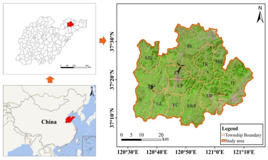
Figure 1.
Location of the study area.
2.2. Data
Sentinel-2 is a high-resolution multispectral imaging satellite carrying a multispectral imager (MSI) with an altitude of 786 km, covering 13 spectral bands with an amplitude of 290 km and ground resolutions of 10 m, 20 m, and 60 m, respectively (Table 1). It is currently the only data containing three bands in the red-edge range, which is effective for monitoring vegetation health [32]. The GEE platform contains two types of Sentinel-2 data: top-of-atmosphere reflectance (TOA) data and surface reflectance (SR) data. The Sentinel-2 L2A-level data in the GEE platform are atmospherically corrected reflectance data, and this study performed mask cloud and cirrus cloud processing for the QA60 band.

Table 1.
Metadata of the Sentinel-2 imagery.
The ground reference data used to train the classification methods and verify the classification results of apple orchard land and other land use types were derived from three sources:
(1) Field survey. The geographical coordinates of each sample point were obtained using handheld GPS (Trimble Geo7x, Sunnyvale, CA, USA), and the corresponding land cover type was recorded in detail. The sample points were evenly distributed throughout the study area, including 40 apple orchard plots, 60 other orchard plots (pear, peach, etc.), and 60 forest and grassland plots. In addition, there are 30 plots of cultivated land, 20 water areas, and 30 construction land plots (Figure 2).
(2) Google Earth images, which have a 2 m spatial resolution.
(3) Auxiliary data. The administrative boundaries of the study area (vector data), land use map and topographic map (raster data), and apple phenology information (Table 2) were obtained from the Qixia government website.
Table 2.
Apple phenology.

Figure 2.
Field sampling distribution.
Figure 2.
Field sampling distribution.

A total of 700 plots were finally collected from the above three sources, including 120 apple orchards, 80 other orchards, 150 cultivated land regions, 150 forest and grassland areas, 100 water areas, and 100 construction land sites.
The DEM data used in basin division and slope analysis were obtained from the Japan Aerospace Exploration Agency’s Advanced Land Observing Satellite-1 (ALOS) topographic data (JAXA). The data were resampled to 10 m from the initial 12.5 m to be consistent with the Sentinel-2 images. The resampled DEM data were then used to extract the basin boundary and slope in the study area.
2.3. Data Processing
The processing flow of the study is shown in Figure 3. All the Sentinel-2 images acquired from 1 March to 30 October were obtained using the GEE platform, and cloud masking was conducted on these data. Four commonly used vegetation indexes, i.e., the Normalized Difference Vegetation Index (NDVI), Soil-Adjusted Vegetation Index (SAVI), Ratio Vegetation Index (RVI), and Difference Vegetation Index (DVI), were then calculated for the feature types in the study area (Table 3), and the optimal temporal phases for identifying apple orchard land were selected based on the variability analysis. After that, the suitable vegetation index, Similar Normalized Difference Building Index (SNDBI), and Similar Normalized Difference Water Index (SNDWI), which can reflect the characteristics of vegetation, artificial surfaces, and water bodies (Table 3), were calculated based on the optimal Sentinel-2 images. All these three indexes, the grayscale co-occurrence matrix, and 70% of the ground reference data were then used as feature variables in the RF classifier for feature information extraction to identify apple orchard land and other feature types, and the SVM extraction results were employed as a comparison.
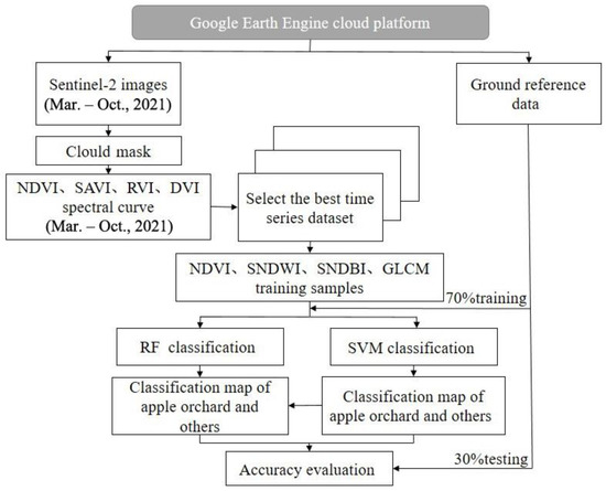
Figure 3.
Workflow of apple orchard land identification.
RF classification is a combination of tree predictors such that each tree depends on the values of a random vector sampled independently and with the same distribution for all trees in the forest [33], which is based on the principles that construct several decision trees. Each decision tree is a classifier, and for an input sample, n trees will have n classification results, and the category with the highest number of votes will be designated as the final output [34]. Among the existing remote sensing classification algorithms, RF information extraction is accurate and efficient, capable of handling input samples with high-dimensional features, and does not require dimensionality reduction to assess the importance of individual features on the classification problem [35]. As a typical nonparametric machine learning algorithm, RF has been successfully applied to crop information identification and mapping for a variety of remote sensing data. In this study, the RF classification was implemented in GEE (ee.Classifier.smileRandomForest). The initial number of trees in the random forest classification model was set to 10. With the increase in the number of trees, the classification accuracies were measured and compared to find the most appropriate number of trees. In this study, 1703 was the optimal number of trees used to identify apple orchard land.
Based on the spectral information of the Sentinel-2 images, the supervised Support Vector Machine (SVM) classification method, a common conventional classification strategy for multispectral images, was used as a comparison to separate the apple orchard areas. It uses hyperplanes to divide pixels into two groups to optimize the distance between the hyperplanes and the closest pixel in each of the two groups [36,37]. The SVM classification algorithms are conducted until a pair of pixels has the closest distance across all classes. In this study, the SVM classification was also implemented in GEE (ee.Classifier.libsvm) using the same training data, the kernelType was RBF, the gamma was set to 0.5, and the cost was 10.
Table 3.
Indexes used in this study.
Table 3.
Indexes used in this study.
| Index | Equation | Reference |
|---|---|---|
| NDVI (Normalized Difference Vegetation Index) | (B8−B4)/(B8 + B4) | [38] |
| SAVI (Soil-Adjusted Vegetation Index) | (1 + L)(B8−B4)/(B8 + B4 + L) L = 0.5 | [39] |
| DVI (Difference Vegetation Index) | B8−B4 | [40] |
| RVI (Ratio Vegetation Index) | B8/B4 | [39] |
| SNDBI (Similar Normalized Difference Building Index) | (B11−B8)/(B11 + B8) | [41] |
| SNDWI (Similar Normalized Difference Water Index) | (B4−B8A)/(B4 + B8A) | [42] |
B11: SWIR 1 band; B8: NIR band; B4: R band.
2.4. Verification
The accuracy of apple orchard land identification can be assessed by a confusion matrix [43]. The proportion of correctly categorized pixels to all pixels is known as the overall accuracy (OA); the user’s accuracy (UA) indicates how many pixels accurately reflect a given class; the producer’s accuracy (PA) indicates how many portions of a given class were correctly represented in the categorized image [44]. Along with the overall consistency between the reference and classified images, the Kappa coefficient () also considers incorrectly classified pixels from the error matrix [45].
where represents the number of rows and columns in the confusion matrix, is the total number of elements, is the elements in row and column , is the marginal total of row , and is the marginal total of column . The Kappa coefficient, which typically ranges from 0 to 1, can be divided into five groups to represent various degrees of consistency: 0.0–0.20 for very low consistency, 0.21–0.40 for average consistency, 0.41–0.60 for moderate consistency, 0.61–0.80 for high consistency, and 0.81–1 for almost perfect consistency.
2.5. Spatial Analysis Methods
The verified apple orchard land results were spatially analyzed using GIS spatial analysis, a slope calculation model, and Moran’s I and Getis-Ord GI* analysis.
The basins and slopes of the study area were calculated using the DEM data (Figure 4a). The study area can be divided into six basins, i.e., the BY (Baiyang River Basin hereinafter), HS (Huangshui River Basin), XH (Xuan River Basin), QY (Qingyang River Basin), QS (Qingshui River Basin), and YC (Yangchu River Basin), based on the hydrology analysis. The slope was classified into six levels, namely, flat slope (Grade I, 0–5°), gentle slope (Grade II, 6–15°), moderate slope (Grade III, 16–25°), steep slope (Grade IV, 26–35°), sharp slope (Grade V, 36–45°), and dangerous slope (Grade VI, >46°), regarding the Second National Land Survey Technical Regulations of China (Figure 4b). The study first converted the apple orchard raster based on RF extraction to vector data, intersected the vector data converted from the slope raster for calculation, and counted the distribution range of apple orchard land with different slopes by basin for spatial mapping and display.
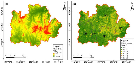
Figure 4.
DEM (a) and slope gradation (b) in the basins of the study area.
Moran’s I and Getis-Ord GI* analysis were employed to analyze the spatial distribution patterns of the apple orchard land in the study area. The Global Moran Index is a measure of the overall clustering of the spatial data [46], and the Local Moran Index calculates the spatial correlation degree between each spatial object in the analysis region and its neighboring objects, analyzes the local characteristic differences in the distribution of spatial objects, and reflects the spatial heterogeneity and instability in the local region [47]. The Global and Local Moran Indexes are defined as:
where is the Global Moran Index measuring global autocorrelation, and is the Local Moran Index; is the number of spatial units indexed by and ; is the variable of interest; is the mean of ; is a matrix of spatial weights with zeroes on the diagonal; and is the sum of all .
The hot spot analysis tool calculates the Getis-Ord Gi* statistic for each feature in a dataset. It is an effective means to explore the characteristics of local spatial clustering distribution, which can distinguish the degree of clustering of variable spatial distribution by cold and hot spots [48]. The Gi* statistic returned for each feature in the dataset is a z-score. For statistically significant positive z-scores, the larger the z-score is, the more intense the clustering of high values (hot spots); the lower the z-score is less than 0, the more intense the clustering of low values (cold spots).
The Getis-Ord local statistic is given as follows:
where is the attribute value for feature , is the spatial weight between feature and , and is the total number of features.
3. Results
3.1. Optimal Time Phase Selection
The NDVI, DVI, RVI, and SAVI for the six land use types (apple orchards, other orchards, cultivated land, construction land, water, and forest and grassland) in the study area during the growing stage of apples (March to October) were depicted in Figure 5. The six land use types can be distinguished using the following time phases.
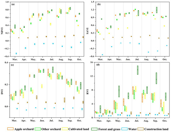
Figure 5.
Vegetation index curves of apple orchard land and other features during the growing stage: (a), NDVI; (b) SAVI; (c) DVI; (d) RVI.
The vegetation index values of water were all less than zero, except the RVI, which was the only land type among the six ones to have index values below zero. For instance, the NDVI value of water in October was the highest among the months, which was from −0.03 to −0.05; the SAVI value of the NDVI in May was −0.08 to −0.09; and the DVI value in May was from −0.008 to −0.01. Similar to the changing pattern of water, the construction land’s NDVI value (less than 0.1), SAVI value (less than 0.14), and DVI value (less than 0.1) in each month were considerably different from those of other land use types. Therefore, it is feasible to distinguish water and construction land from vegetation using the three vegetation indexes.
The vegetation indexes of forest and grassland have the highest values in the majority of the months (Figure 5). Although the SAVI and DVI in each month have obvious overlaps with apple orchard land and other orchard lands, the NDVI values of forest and grassland in March, April, May, and October are distinguishable from them.
For cultivated land, the NDVI and SAVI in April (0.21–0.24, 0.28–0.3), May (0.62–0.65, 0.45–0.48), July (0.4–0.45, 0.97–1.16), and October (0.38–0.4, 0.56–0.59) have clear low values that can be used to recognize it.
To separate apple orchards and other orchards, the ranges of NDVI values in April (0.3–0.33, 0.25–0.295), May (0.52–0.58, 0.43–0.48), June (0.6–0.7, 0.52–0.55), and October (0.61–0.66, 0.5–0.53) have few overlaps; it was more likely to correctly identify apple orchard land during these four months.
In summary, April, May, and October were the optimal time phases for apple orchard land identification, and the NDVI can classify different types of land cover more accurately than other indexes. Therefore, the Sentinel-2 images and NDVI results acquired in these three months were subsequently processed and analyzed.
3.2. Verification of Apple Orchard Land Identification
Figure 6 displays the results of the land system in the study area based on the RF and SVM methods. The confusion matrix was constructed using the ground reference set to verify the extraction results of the RF and SVM methods, which were shown in Table 4 and Table 5.
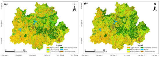
Figure 6.
Classification map based on the RF (a) and SVM (b) classification methods.
Table 4.
Confusion matrix of the RF method using 210 verification plots.
Table 5.
Confusion matrix of the SVM method using 210 verification plots.
The overall accuracy (90%) of the RF classification results was 9.2% higher than that of the SVM extraction results and so was the Kappa coefficient (0.88, increased by 11.4%). The lowest production accuracy of the SVM method was 56.5% for the other orchard, and the lowest production accuracy of the RF method also occurred in the other orchard extraction (77.8%), which may be related to the fact that spectral and texture information were inconsistent among the other orchards within the land class; the production accuracy of apple orchard land identification (93.1%) was improved by 25.6% compared with that extracted by the SVM method (74.2%). Overall, the producer’s and user’s accuracies of the RF method were all higher than those of the SVM method; RF is more suitable for apple orchard land identification than the generic SVM classification method.
3.3. Spatial Distribution of Apple Orchard Land
The distribution of apple orchard land in the study area obtained based on the RF classification method is shown in Figure 7. The total distribution of apple orchard land in the study area is 485.8 km2 (Table 6), which is 0.6% less than the 488.6 km2 in the government statistical yearbook from the field survey [49].
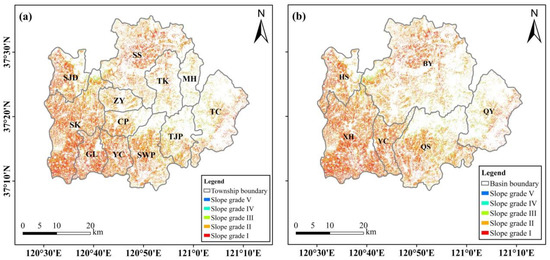
Figure 7.
Spatial distribution of apple orchard land in the study area by township and slope (a) and basin and slope (b).
Table 6.
Area of the apple orchard in different towns and slope grades.
The distribution patterns of apple orchard land in the study area varied across slope grades. Similar to the pattern found in the field investigation, there was no apple orchard land distributed on the dangerous slope (Grade VI, >46°). More than half (55.7%) of the apple orchard land was located on the gentle slope (Grade II, 6–15°) and 35.3% on the flat slope (Grade I, 0–5°), which supported more than 90% of the apple orchards. Only 8.2% was distributed on the moderate slope (Grade III, 16–25°), as shown in Figure 8a. A total of 4.2 km2 (0.9%) of apple orchard land was distributed on the steep slope (Grade IV, 26–35°) and sharp slope (Grade V, 36–45°), as shown in Figure 8b.
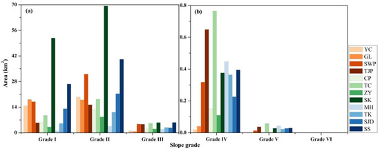
Figure 8.
(a,b) Patterns of apple orchards by township and slope. YC: Yangchu (hereinafter), GL: Guanli, SWP: Shewopo, TJP: Tangjiapo, CP: Cuiping, TC: Taocun, ZY: Zhuangyuan, SK: Sikou, MH: Miaohou, TK: Tingkou, SJD: Sujiadian, SS: Songshan.
At the township scale, SK occupied the highest area proportion of apple orchard land (127.2 km2), accounting for 26.2% of the total area in the study area, then SS (72.9 km2, 15.0%) and SWP (54.2 km2, 11.2%). These three towns contained more than 50% of the total orchard area. The ratios of the other 12 towns were all lower than 10%, and the lowest proportion was 1.4% (6.9 km2) in MH (Figure 8 and Table 6). At different slope grades, the spatial distribution of apple orchard land in each basin was consistent with the overall characteristics: there were no apple orchards distributed on the dangerous slope (Grade VI, >46°). On the sharp slope (Grade V, 36–45°), all the towns have little distribution. Apple orchards were mainly distributed on the gentle slope (Grade II, 6–15°), with the highest percentage of apple orchard land in SK (25.6%) and the lowest in MH (1.3%); on the flat slope (Grade I, 0–5°), the highest percentage of apple orchard land was distributed in SK (30.2%) and the lowest in MH (0.6%).
At the basin scale, the XH had the largest apple orchard area (152.5 km2), then the BY (128 km2) and the QS (92.3 km2); the QY had the smallest apple orchard area (Table 7). At different slope grades, the spatial distribution of apple orchard land in each basin was consistent with the overall characteristics: there was no apple orchard distributed on the dangerous slope (Grade VI, >46°). On the sharp slope (Grade V, 36–45°), QH has the smallest apple orchard land distribution, and the other basins have very little distribution (Figure 9 and Table 7). Apple orchard land was mainly distributed on the gentle slope (Grade II, 6–15°), with the highest percentage of apple orchards in the QS (58.5%) and the lowest in the XH, but still higher than 50% (52.7%); on the flat slope (Grade I, 0–5°), the highest percentage of apple orchards was distributed in the QH (44.1%) and the lowest in the QS (29.3%).
Table 7.
Area of the apple orchard land in different basins and slope grades.
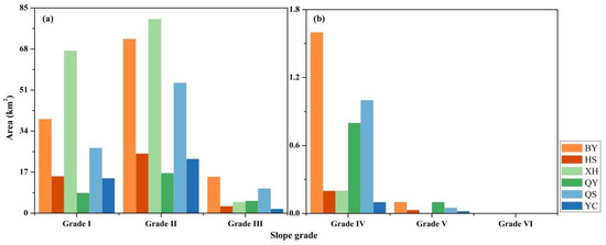
Figure 9.
(a,b) Patterns of apple orchard land by basin and slope. BY: Baiyang River Basin, HS: Huangshui River Basin), XH: Xuan River Basin, QY: Qingyang River Basin, QS: Qingshui River Basin, YC: Yangchu River Basin.
3.4. Moran’s I and Getis-Ord GI* Analysis
Moran’s I and Getis-Ord GI* analysis were applied to the apple orchard areas in 954 counties of the 12 towns in the study area (Table 8), as they were not applicable at the township scale. Global Moran’s I computation results demonstrated that the distribution of apple orchard land has a positive spatial autocorrelation (0.309, p = 0.000). Local Moran’s I analysis showed that not-significant cluster types prevailed in the study area (467 of 954), which were in all the towns. A total of 130 counties exhibited a High–High cluster type, which were located in SK, YC, SWP, GL, SJD, TJP, and SS, from high to low. Among these seven towns, SK contained 60% of the High–High cluster counties, which was the most; SS only contained one High–High cluster county. A total of 25 counties in seven 7 towns (SS, TC, ZY, TK, MH, TJP, and CP) showed a High–Low cluster type, which was the lowest account among the five cluster types. In this category, SS contained the most counties (10), and TJP, CY has 1 county, respectively. A total of 59 counties in seven towns (SK, GL, SJD, YC, SWP, CP, and SS) displayed a Low–High cluster type, in which SK ranked first with 28 counties. Different from the other three types, 273 counties showed a Low–Low type in eight towns (TC, TK, CP, TJP, SS, ZY, MH, and SWP), and TC and TK ranked the first and second, respectively (Figure 10a).
Table 8.
Cluster types using Local Moran’s I in the study area.
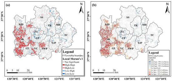
Figure 10.
Local Moran’s I (a) and Getis-Ord GI* (b) of apple orchard land in the study area.
The Getis-Ord GI* analysis was used to detect cold and hot spots of apple orchard land areas in the study area. Figure 10b showed whether the spatial clustering of the sampling sites was significant and, if so, at what level (0.01, 0.05, and 0.1 levels). The spatial weight matrix was calculated based on the Euclidean distance between sampling sites, and the distance threshold was 3140.682 m. The spatial heterogeneity analysis found that 243 hot spots were mainly located in SK, SJD, GL, YC, SWP, and TJP; 293 cold spots were distributed in ZY, CP, TJP, TC, TK, MH, and SS. The distribution patterns of cold and hot spots converged with those of the Local Moran Index computation results.
4. Discussion
This is the first study that combined multitemporal Sentinel-2 images and the RF classification method to explore a new framework to efficiently identify and monitor apple orchard land. The results found that April, May, and October were the optimal time phases for apple orchard identification, the RF-based method can accurately identify apple orchard land with high accuracies, apple orchard land showed diverse distribution patterns in different towns and basins, and the distribution of apple orchard land has a positive spatial autocorrelation. The distribution patterns of cold and hot spots converged with those of the Local Moran Index computation results.
Compared to single-temporal images, multitemporal images can provide more spectral information about crops in different growth stages [50], which can help reduce classification errors and improve the accuracy of crop identification. In this study, the values of vegetation indexes of all the land types were high (e.g., 0.78 for apple orchard land and 0.75 for other orchard lands) in summer (Figure 5), but they overlapped and overwhelmed each other; in spring and autumn, the land types overlapped less and were highly distinguished. Therefore, this study proposed that Sentinel-2 images based on April, May, and October are suitable to identify apple orchard land from other vegetation areas. Among the existing studies, Dai used multitemporal high-resolution remote sensing images to identify apple orchard land in northwest China and proposed that April was the best time phase for identifying apple orchard land [18]; Dong proposed that apple orchard land be identified in April and May during the flowering period [51]; Xu presented that apple orchard land identification accuracy was the highest in October [52]. The temporal stages involved in these studies are consistent with the findings of this study.
The top fifteen characteristics in terms of feature relevance were chosen for the RF classification procedure and ranked according to the magnitude of contribution. Different from the results found in existing studies (e.g., [16,18]), the texture information did not contribute prominently compared to the indexes and band spectral information. As shown in Figure 11, the first place among the top fifteen characteristics was taken by the NDVI contribution of Sentinel-2 images in October. It can be found in Figure 5 that the NDVI of each land use type overlapped each other in October. The NDVI is a crucial indicator reflecting orchard growth: the more lush the orchard, the higher the NDVI value. In contrast to other orchards, apple orchard land in the study area was in the maturation stage in October. Cultivated land was in the sowing stage, and the NDVI was at a low value. Forest and grassland began to shed their leaves at this time. Thus, during this time, apple orchard land can be distinguished by the NDVI. Other significant identification features are the NDVI in April, SNDWI in May, SNDWI, and SNDBI in October. Considering the band information, the green light band (B3) of the images in April also had a high contribution. In April, apple orchard land and other orchards were in the blossoming stage, which could be recognized from other feature types. In addition, the blue (B2) and red-edge bands (B6, B7, Table 1) also contributed to apple orchard land identification. This is because the Sentinel-2 image is currently the sole data form that has three red-edge bands, which is effective for vegetation health monitoring. This implies that the Sentinel-2 image is the optimal data for apple orchard land identification and monitoring.
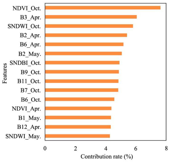
Figure 11.
Contribution of each feature in the RF method.
The identification accuracy of apple orchard land based on the RF classifier was acceptable in this study, while the production accuracy and user accuracy of other orchards were relatively low (77.8%). There are pear orchards, peach orchards, cherry orchards, and vineyards, in addition to walnut and chestnut orchards planted in the study area [53]. The types of these orchards are complex and influenced by topographic and slope factors, which are prone to be confused with cultivated and forest and grassland types (Table 4). Therefore, the accuracy of extracting structures by combining them with other orchards is not that high. The production and user accuracies of other feature types, such as watershed, construction land, and forest grassland are around 90%, indicating that the proposed algorithm has a high recognition rate for spectrally stable and uniform texture features.
The spatial analysis found that more than half (55.7%) of the apple orchard land was distributed on the gentle slope (Grade II, 6–15°). However, 171.5 km2 (35.3%) of apple orchards were found to distribute on the flat slope (Grade I, 0–5°). According to China’s policy on cultivated land protection, the flat slope areas should be given primary priority for cultivating arable land and grain crops. However, to generate a scale effect and boost the annual income, more farmers are converting cultivated land into apple orchard land, which induced the decropping of cultivated land [54,55]. As the spatialized data of cultivated land decropping are temporally lacking, the results obtained from this study can serve as a reference for policymakers to form more targeted regulations and policies.
In this study, an apple orchard land identification method was explored using multitemporal Sentinel-2 images, while this study has limitations. Firstly, there have been studies on the use of new methods, such as artificial neural network particle swarm optimization [56], machine learning with an empirical Bayesian Kriging interpolation method [57], and deep learning methods, such as MANet [58] and MLNet [59], for the extraction of land use types. Further study can be conducted to explore the feasibility of these methods to identify apple orchard land. Secondly, accurate ground reference data are crucial for training and validating the classification algorithm [60]. Due to the lockdown policy during the COVID-19 epidemic period and the topographical impact in the study area, they were temporally unavailable to collect more field reference data. As most of the training data were obtained from Google Earth images based on visual interpretation, uncertainty may be introduced in the final classification results. More field surveys will be conducted in the future study to cover the entire study area. Thirdly, the historical data of GEE data are temporarily unavailable in some regions (e.g., mainland China), and one-year images were used in this study for exploratory research. In the future study, more data sources, such as UAV images and WorldView historical images, will be combined to analyze the time-series change patterns of apple orchard land.
5. Conclusions
Using multitemporal Sentinel-2 images and the RF classification method on the GEE platform, this study investigated the optimal identification time phases and spatial distribution monitoring of apple orchard land. The findings showed that the Sentinel-2 images acquired in April, May, and October were suitable for accurate information extraction regarding apple orchard land using the vegetation, building, and water indexes, which can maximize the advantages of Sentinel-2 images’ band setting. The identification accuracies are high with the overall accuracy and Kappa coefficient reaching 90% and 0.88, increased by 9.2% and 11.4%, respectively, compared to the results using the SVM method. The distribution patterns of apple orchard land varied in townships and on slopes, as well as in basins and on slopes. More than 90% of apple orchards were spread on the gentle slope (Grade II, 6–15°) and flat slope (Grade I, 0–5°). The distribution of apple orchard land has a positive spatial autocorrelation (0.309, p = 0.000). High–High, High–Low, Low–High, and Low–Low cluster types occurred mainly in Sikou (60%), (47.5%), Taocun, and Tingkou (37.4%), respectively. The distribution patterns of cold and hot spots converged with those of the Local Moran Index computation results. More field measurement data will be incorporated in future studies to increase the extraction accuracy of apple orchard land and more image data sources will be combined to fully detect time-series changes in apple orchards. The findings can be utilized as references for future orchard information extraction and monitoring.
Author Contributions
Conceptualization, X.Z. and X.Y.; software, X.T.; validation, Y.Y.; field investigation, Y.Y. and X.T.; writing—original draft, X.Y. and X.T.; writing—review and editing, X.Y. and X.Z. All authors have read and agreed to the published version of the manuscript.
Funding
This study was supported by the National Natural Science Foundation of China (grant No. 42171378 and 41671346), and the National Key Research and Development Program of China (2022YFC3204404). The supporters had no role in the study design, data collection, analysis, decision to publish, or preparation of the manuscript.
Data Availability Statement
Data used in this study are available under request.
Acknowledgments
We would like to thank the kind help of the editor and the reviewers to improve the manuscript.
Conflicts of Interest
The authors declare no conflict of interest.
References
- Frolking, S.; Qiu, J.; Boles, S.; Xiao, X.; Liu, J.; Zhuang, Y.; Li, C.; Qin, X. Combining remote sensing and ground census data to develop new maps of the distribution of rice agriculture in China. Glob. Biogeochem. Cycles 2002, 16, 38-1–38-10. [Google Scholar] [CrossRef]
- Nabi, F.; Jamwal, S.; Padmanbh, K. Wireless sensor network in precision farming for forecasting and monitoring of apple disease: A survey. Int. J. Inf. Technol. 2020, 14, 769–780. [Google Scholar] [CrossRef]
- Wang, J.; Xiao, X.; Liu, L.; Wu, X.; Qin, Y.; Steiner, J.L.; Dong, J. Mapping sugarcane plantation dynamics in Guangxi, China, by time series Sentinel-1, Sentinel-2 and Landsat images. Remote Sens. Environ. 2020, 247, 111951. [Google Scholar] [CrossRef]
- Ruscica, R.C.; Polcher, J.; Salvia, M.M.; Sörensson, A.A.; Piles, M.; Jobbágy, E.G.; Karszenbaum, H. Spatio-temporal soil drying in southeastern South America: The importance of effective sampling frequency and observational errors on drydown time scale estimates. Int. J. Remote. Sens. 2020, 41, 7958–7992. [Google Scholar] [CrossRef]
- Ballesteros, R.; Ortega, J.F.; Hernandez, D.; del Campo, A.; Moreno, M.A. Combined use of agro-climatic and very high-resolution remote sensing information for crop monitoring. Int. J. Appl. Earth Obs. Geoinf. 2018, 72, 66–75. [Google Scholar] [CrossRef]
- Ghamisi, P.; Rasti, B.; Yokoya, N.; Wang, Q.; Hofle, B.; Bruzzone, L.; Benediktsson, J.A. Multisource and multitemporal data fusion in remote sensing: A comprehensive review of the state of the art. IEEE Geosci. Remote Sens. Mag. 2019, 7, 6–39. [Google Scholar] [CrossRef]
- Ghorbanian, A.; Ahmadi, S.A.; Amani, M.; Mohammadzadeh, A.; Jamali, S. Application of Artificial Neural Networks for Mangrove Mapping Using Multi-Temporal and Multi-Source Remote Sensing Imagery. Water 2022, 14, 244. [Google Scholar] [CrossRef]
- Reuß, F.; Greimeister-Pfeil, I.; Vreugdenhil, M.; Wagner, W. Comparison of long short-term memory networks and random forest for sentinel-1 time series based large scale crop classification. Remote Sens. 2021, 13, 5000. [Google Scholar] [CrossRef]
- Meshram, P.; Ray, S.S. Field-level crop classification using an optimal dataset of multi-temporal sentinel-1 and polarimetric RADARSAT-2 SAR data with machine learning algorithms. J. Indian Soc. Remote Sens. 2021, 49, 2945–2958. [Google Scholar]
- Zhang, X.; Xiong, Q.; Di, L.; Tang, J.; Yang, J.; Wu, H.; Qin, Y.; Su, R.; Zhou, W. Phenological metrics-based crop classification using HJ-1 CCD images and Landsat 8 imagery. Int. J. Digit. Earth 2018, 11, 1219–1240. [Google Scholar] [CrossRef]
- Qiu, B.; Luo, Y.; Tang, Z.; Chen, C.; Lu, D.; Huang, H.; Chen, Y.; Chen, N.; Xu, W. Winter wheat mapping combining variations before and after estimated heading dates. ISPRS J. Photogramm. Remote. Sens. 2017, 123, 35–46. [Google Scholar] [CrossRef]
- Moumni, A.; Oujaoura, M.; Ezzahar, J.; Lahrouni, A. A new synergistic approach for crop discrimination in a semi-arid region using Sentinel-2 time series and the multiple combination of machine learning classifiers. J. Physics Conf. Ser. 2021, 1743, 012026. [Google Scholar] [CrossRef]
- Pluto-Kossakowska, J.; Pilarska, M.; Bartkowiak, P. Automatic detection of dominant crop types in poland based on satellite images. Artif. Satell. 2020, 55, 185–208. [Google Scholar] [CrossRef]
- Hunt, M.L.; Blackburn, G.A.; Carrasco, L.; Redhead, J.W.; Rowland, C.S. High resolution wheat yield mapping using Sentinel-2. Remote Sens. Environ. 2019, 233, 111410. [Google Scholar] [CrossRef]
- D’Amico, G.; Francini, S.; Giannetti, F.; Vangi, E.; Travaglini, D.; Chianucci, F.; Mattioli, W.; Grotti, M.; Puletti, N.; Corona, P.; et al. A deep learning approach for automatic mapping of poplar plantations using Sentinel-2 imagery. GIScience Remote Sens. 2021, 58, 1352–1368. [Google Scholar] [CrossRef]
- Yue, J.; Wang, Z.; Feng, Z. Remote sensing identification of fruit tree species in Southern Xinjiang Basin based on spectral and texture characteristics. J. Xinjiang Agric. Univ. 2015, 38, 326–333. [Google Scholar]
- Qin, Q.; Wang, B.; Li, F.; Wang, H.; Zhao, H.; Shu, M. Object-oriented Remote sensing extraction of apple tree planting area from GF-1 satellite image: A case study of Qixia City in hilly region. Meteorol. Desert Oasis 2020, 2, 129–136. [Google Scholar]
- Dai, J. Apple orchard extraction based on high score and multi-temporal image segmentation. Agric. Resour. Reg. China 2022, 8, 140–148. [Google Scholar]
- Paul, S.; Kumar, D.N. Evaluation of feature selection and feature extraction techniques on multi-temporal landsat-8 images for crop classification. Remote Sens. Earth Syst. Sci. 2019, 2, 197–207. [Google Scholar] [CrossRef]
- Chen, B.; Xiao, X.; Li, X.; Pan, L.; Doughty, R.; Ma, J.; Giri, C. A mangrove forest map of China in 2015: Analysis of time series Landsat 7/8 and Sentinel-1A imagery in Google Earth Engine cloud computing platform. ISPRS J. Photogramm. Remote Sens. 2017, 131, 104–120. [Google Scholar] [CrossRef]
- Tuvdendorj, B.; Zeng, H.; Wu, B.; Elnashar, A.; Zhang, M.; Tian, F.; Natsagdorj, N. Performance and the optimal integration of sentinel-1/2 time-series features for crop classification in northern mongolia. Remote Sens. 2022, 14, 1830. [Google Scholar] [CrossRef]
- Luo, Y.; Zhang, Z.; Zhang, L.; Han, J.; Cao, J.; Zhang, J. Developing high-resolution crop maps for major crops in the european union based on transductive transfer learning and limited ground data. Remote Sens. 2022, 14, 1809. [Google Scholar] [CrossRef]
- Bangira, T.; Alfieri, S.M.; Menenti, M.; van Niekerk, A. Comparing thresholding with machine learning classifiers for mapping complex water. Remote Sens. 2019, 11, 1351. [Google Scholar] [CrossRef]
- Rani, A.; Kumar, N.; Sinha, N.K.; Kumar, J. Identification of salt-affected soils using remote sensing data through random forest technique: A case study from India. Arab. J. Geosci. 2022, 15, 381. [Google Scholar] [CrossRef]
- Hamimeche, M.; Niculescu, S.; Billey, A.; Moulaï, R. Identification and mapping of Algerian island vegetation using high-resolution images (Pléiades and SPOT 6/7) and random forest modeling. Environ. Monit. Assess. 2021, 193, 617. [Google Scholar] [CrossRef]
- Wang, Y.; Li, Y.; Song, Y.; Rong, X. Facial expression recognition based on random forest and convolutional neural network. Information 2019, 10, 375. [Google Scholar] [CrossRef]
- Zhao, W.-F.; Xiong, L.-Y.; Ding, H.; Tang, G.-A. Automatic recognition of loess landforms using Random Forest method. J. Mt. Sci. 2017, 14, 885–897. [Google Scholar] [CrossRef]
- Lebourgeois, V.; Dupuy, S.; Vintrou, É.; Ameline, M.; Butler, S.; Bégué, A. A combined random forest and OBIA classification scheme for mapping smallholder agriculture at different nomenclature levels using multisource data (simulated Sentinel-2 time series, VHRS and DEM). Remote Sens. 2017, 9, 259. [Google Scholar] [CrossRef]
- Ok, A.O.; Akar, O.; Gungor, O. Evaluation of random forest method for agricultural crop classification. Eur. J. Remote Sens. 2012, 45, 421–432. [Google Scholar] [CrossRef]
- Zhou, L.; Dang, X.; Sun, Q.; Wang, S. Multi-scenario simulation of urban land change in Shanghai by random forest and CA-Markov model. Sustain. Cities Soc. 2020, 55, 102045. [Google Scholar] [CrossRef]
- Wu, H.; Lin, A.; Xing, X.; Song, D.; Li, Y. Identifying core driving factors of urban land use change from global land cover products and POI data using the random forest method. Int. J. Appl. Earth Obs. Geoinf. 2021, 103, 102475. [Google Scholar] [CrossRef]
- Drusch, M.; Del Bello, U.; Carlier, S.; Colin, O.; Fernandez, V.; Gascon, F.; Bargellini, P. Sentinel-2: ESA’s optical high-resolution mission for GMES operational services. Remote Sens. Environ. 2012, 120, 25–36. [Google Scholar] [CrossRef]
- Breiman, L. Random forests. Mach. Learn. 2001, 45, 5–32. [Google Scholar] [CrossRef]
- Belgiu, M.; Drăguţ, L. Random forest in remote sensing: A review of applications and future directions. ISPRS J. Photogramm. Remote Sens. 2016, 114, 24–31. [Google Scholar] [CrossRef]
- Teluguntla, P.; Thenkabail, P.S.; Oliphant, A.; Xiong, J.; Gumma, M.K.; Congalton, R.G.; Huete, A. A 30-m landsat-derived cropland extent product of Australia and China using random forest machine learning algorithm on Google Earth Engine cloud computing platform. ISPRS J. Photogramm. Remote Sens. 2018, 144, 325–340. [Google Scholar] [CrossRef]
- Ding, S.; Zhang, X.; Yu, J. Twin support vector machines based on fruit fly optimization algorithm. Int. J. Mach. Learn. Cybern. 2016, 7, 193–203. [Google Scholar] [CrossRef]
- Vapnik, V. The Nature of Statistical Learning Theory; Springer Science & Business Media: Berlin, Germany, 1999. [Google Scholar]
- Xue, J.; Su, B. Significant remote sensing vegetation indices: A review of developments and applications. J. Sens. 2017, 2017, 1353691. [Google Scholar] [CrossRef]
- Huete, A.R. A soil-adjusted vegetation index (SAVI). Remote Sens. Environ. 1988, 25, 295–309. [Google Scholar] [CrossRef]
- Perry, C.R., Jr.; Lautenschlager, L.F. Functional Equivalence of Spectral Vegetation Indices; Johnson Space Center: Houston, TX, USA, 1983. [Google Scholar]
- Zha, Y.; Gao, J.; Ni, S. Use of normalized difference built-up index in automatically mapping urban areas from TM imagery. Int. J. Remote Sens. 2003, 24, 583–594. [Google Scholar] [CrossRef]
- DeMets, S.A.; Ziemann, A.; Manore, C.; Russell, C. Too Big, too Small, or just Right? The influence of multispectral image size on mosquito population predictions in the greater Toronto area. In Proceedings of the Algorithms, Technologies, and Applications for Multispectral and Hyperspectral Imagery XXVI, Online, 12–16 May 2020; SPIE: Bellingham, WA, USA, 2020; Volume 11392, pp. 224–231. [Google Scholar]
- Gongal, A.; Silwal, A.; Amatya, S.; Karkee, M.; Zhang, Q.; Lewis, K. Apple crop-load estimation with over-the-row machine vision system. Comput. Electron. Agric. 2016, 120, 26–35. [Google Scholar] [CrossRef]
- Tung, F.; LeDrew, E. The determination of optimal threshold levels for change detection using various accuracy indexes. Photogramm. Eng. Remote Sens. 1988, 54, 1449–1454. [Google Scholar]
- Rosenfield, G.H.; Fitzpatrick-Lins, K. A coefficient of agreement as a measure of thematic classification accuracy. Photogramm. Eng. Remote Sens. 1986, 52, 223–227. [Google Scholar]
- Moran, P.A. Notes on continuous stochastic phenomena. Biometrika 1950, 37, 17–23. [Google Scholar] [CrossRef] [PubMed]
- Anselin, L. Local indicators of spatial association—LISA. Geogr. Anal. 1995, 27, 93–115. [Google Scholar] [CrossRef]
- Getis, A.; Ord, J.K. The Analysis of Spatial Association by Use of Distance Statistics. In Perspectives on Spatial Data Analysis; Springer: Berlin/Heidelberg, Germany, 2009; pp. 127–145. [Google Scholar]
- Qixia Municipal Bureau of Statistics. Qixia Statistical Yearbook for the Year 2021; Qixia Bureau of Statistics: Qixia, China, 2022.
- Vuolo, F.; Neuwirth, M.; Immitzer, M.; Atzberger, C.; Ng, W.-T. How much does multi-temporal Sentinel-2 data improve crop type classification? Int. J. Appl. Earth Obs. Geoinf. 2018, 72, 122–130. [Google Scholar] [CrossRef]
- Dong, F.; Zhao, G.; Wang, L.; Zhu, X.; Lei, T. Remote sensing extraction technique for apple orchards based on hybrid image element decomposition of measured spectra. J. Appl. Ecol. 2012, 23, 3361–3368. [Google Scholar]
- Xu, L.; Lv, J. Recognition method for apple fruit based on SUSAN and PCNN. Multimed. Tools Appl. 2018, 77, 7205–7219. [Google Scholar] [CrossRef]
- Wei, S.; Wang, S. Effects of bagging on aroma of qixia pear fruit. Agric. Sci. Technol. 2015, 16, 1676. [Google Scholar]
- Liu, Z.; Ma, P.; Zhai, B.; Zhou, J. Soil moisture decline and residual nitrate accumulation after converting cropland to apple orchard in a semiarid region: Evidence from the loess plateau. Catena 2019, 181, 104080. [Google Scholar] [CrossRef]
- Wang, J.; Liu, Y.; Liu, Z. Spatio-temporal patterns of cropland conversion in response to the “grain for green project” in China’s loess hilly region of Yanchuan County. Remote Sens. 2013, 5, 5642–5661. [Google Scholar] [CrossRef]
- Alizamir, M.; Sobhanardakani, S. An artificial neural network-particle swarm optimization (ANN-PSO) approach to predict heavy metals contamination in groundwater resources. Jundishapur J. Health Sci. 2018, 10, e67544. [Google Scholar] [CrossRef]
- Senoro, D.B.; de Jesus, K.L.M.; Mendoza, L.C.; Apostol, E.M.D.; Escalona, K.S.; Chan, E.B. Groundwater quality monitoring using in-situ measurements and hybrid machine learning with empirical bayesian kriging interpolation method. Appl. Sci. 2021, 12, 132. [Google Scholar] [CrossRef]
- Chen, B.; Xia, M.; Qian, M.; Huang, J. MANet: A multi-level aggregation network for semantic segmentation of high-resolution remote sensing images. Int. J. Remote Sens. 2022, 43, 5874–5894. [Google Scholar] [CrossRef]
- Gao, J.; Weng, L.; Xia, M.; Lin, H. MLNet: Multichannel feature fusion lozenge network for land segmentation. J. Appl. Remote Sens. 2022, 16, 016513. [Google Scholar] [CrossRef]
- Jin, Z.; Azzari, G.; You, C.; Di Tommaso, S.; Aston, S.; Burke, M.; Lobell, D.B. Smallholder maize area and yield mapping at national scales with Google Earth Engine. Remote Sens. Environ. 2019, 228, 115–128. [Google Scholar] [CrossRef]


Disclaimer/Publisher’s Note: The statements, opinions and data contained in all publications are solely those of the individual author(s) and contributor(s) and not of MDPI and/or the editor(s). MDPI and/or the editor(s) disclaim responsibility for any injury to people or property resulting from any ideas, methods, instructions or products referred to in the content. |
© 2023 by the authors. Licensee MDPI, Basel, Switzerland. This article is an open access article distributed under the terms and conditions of the Creative Commons Attribution (CC BY) license (https://creativecommons.org/licenses/by/4.0/).