Abstract
The flood peak is commonly estimated using the rational method for the design of hydraulic structures. The method is mainly used in a deterministic context. However, there is often uncertainty in flood predictions, which should be incorporated in the design of mitigation schemes. This research proposes a methodology to cope with uncertainty in the rational method via the application of a stochastic framework. Data from 158 storms, recorded in the period 1984–1987 in 19 subbasins in the southwestern part of Saudi Arabia, were used to implement the proposed methodology. A tri-variate log-normal probability density function was used to model the joint relationship between the rational method parameters. The model considered the parameters as random variables. The uncertainty in the rainstorms was represented by intensity or depth; the uncertainty in basin delineation (due to the use of different digital elevation model resolution) was represented by the basin area; and the uncertainty in the land use/land cover was represented by the runoff coefficient. The Monte Carlo method was used to generate realizations of the peak flow and runoff volume with 95% and 99% confidence levels from the input parameters. Although the correlation between the parameters was weak, the model was capable of simulating the rational model parameters and estimating the peak flow and runoff volume relatively well, and the generated realizations fell within the confidence levels, except for a few marginal cases. The model can be used to generate peak flows and the associated confidence limits in ungauged basins from the statistics of the input parameters using the equations developed in this study.
1. Introduction
Climate change in the Kingdom of Saudi Arabia (KSA) has been reflected in terms of the frequency and severity of flooding [1]. These changes have resulted in massive floods that have caused a great loss of property and human lives despite the improved infrastructure, the installed forecasting systems, and new urban planning and management. The magnitude of recent floods has impacted the society and led to an urgent need to address flood hazards using an integrated approach. On the other hand, extensive, rapid, and intense development is currently underway in the KSA as a result of Version 2030. New major cities and expansion areas have been and are being developed in flood-prone areas. As a result, the government has mandated flood studies as a requirement for all construction projects, regardless of size.
In addition, Saudi Arabia is located in arid areas. It is well-known that arid areas suffer from variable rainfall and losses, a decline in vegetation, and a high rate of erosion. Zero flows prevail in stream networks most days of the year [2,3]. Infrequent flooding usually occurs as a result of high-intensity storms in a smaller portion of the watershed. The variability of flooding varies greatly from year to year and from site to site.
Moreover, there is a lack of high-quality runoff data and broad-based flood estimation methods in these regions [4,5]. Therefore, the use of simple design methods has become necessary for estimating floods, as the use of design methods that require a large amount of data is not feasible and impractical [6,7]. Many studies have used the rational method because of its simplicity and reliance on a few data.
The rational formula dates back to the 1850s [8]. Because of its simplicity and limited data requirements, the method is still widely applied in estimating the peak runoff discharge of a small watershed responding to a storm [9]. The rational method (RM) is the most commonly used technique to determine the maximum runoff volumes for the design of urban drainage infrastructure [10]. The method was developed under the assumption that rainfall intensity is uniformly distributed in time and space, and so are the losses or infiltration losses. The traditional rational method is generally used, provided that the duration of the precipitation storm, D, is equal to or greater than the concentration–time, tc, to obtain the design peak discharge with design frequency [11].
The literature review shows that there are large number of studies that have investigated this method. Titmarsh et al. [12] studied the values of the main parameter of two simple flood estimation models, the runoff coefficient in the rational method and the curve number in the Soil Conservation Service (SCS) method. Both parameters were derived from 105 small agricultural catchments in Australia. The results show that the values from the conventional manual differed from the derived values as the former yielded inaccurate estimates of runoff volume and flood peaks. In addition, the average recurrence interval and method of estimating the design rainfall period were found to have a greater influence on the derived values than the land use and soil type. Chin [13] used the rational method based on intensity–duration–frequency (IDF) curves to assess the hypothesis that the maximum peak runoff discharge occurs as the duration of constant rainfall intensity is equal to the concentration time. Their results showed that the peak runoff discharge was underestimated when the constant rainfall intensity was estimated by a duration equal to the concentration time.
In applying the traditional rational method, only the peak runoff discharge (Qp) is obtained. However, in many cases, not only is the Qp needed, but the volume and the runoff hydrograph for design are also required. Therefore, many modifications have been made to the rational method to produce runoff hydrographs such as revisiting the rational method for flood estimation in the Saudi Arabian environment to investigate the validity of applying the method in large catchments in arid regions [14]. The authors in [14] extended the method to capture not only Qp, but also the runoff volume. A total of 160 storms recorded during the period 1984–1987 were analyzed in 19 sub-catchments ranging in size from 170 to 4930 km2 in southwestern Saudi Arabia. It was found that the rational method is not only limited to estimating the peak flows for small catchments (less than 5 km2), as mentioned in the literature, but also provides very good matches with the observations of peak discharges and volumes for larger catchments.
Dhakal et al. [15] applied the modified RM method to 90 catchments in Texas. It was found that the method could be applied to catchments that exceeded the classical limit of a few hundred acres. The method also obtained results not far from other unit hydrograph methods. However, the application of the RM, in a deterministic sense, needs the prerequisites of great experience and engineering judgment when applying this simple method.
Young, et al. [16] investigated the dependence of the runoff coefficient, C, on the recurrence interval. The C values for 72 gauged rural Kansas catchments with areas in the range between 0.45 and 76.6 km2 were tested using the common frequency approach. They showed a dependence of C on the recurrence interval, however, there was no dependence on the drainage area, indicating that the method can be used for much larger catchments.
There is substantial uncertainty in the results of the rational method, which is due to inherent uncertainties in the estimation of the input parameters [17], therefore, in this research, we targeted this point.
The general objective of this study was to quantify the uncertainty that exists in the modeling of hydrological basins while applying the simplest hydrological model, namely, the rational method. The more specific objectives are: (1) to formulate the rational method in a stochastic context rather than in the traditional deterministic one using the tri-variate log-normal distribution of the rational method parameters (rainfall intensity or rainfall depth, basin area, and runoff coefficient); (2) to apply the Monte Carlo (MC) method to quantify the uncertainty in the rational method (i.e., estimation of the variance of the peak flow and volume as a function of the variance of the rational method parameters); and (3) to compare the results of the MC method with the analytical method based on the first-order second-moment (FOSM) for the rational method developed by the authors in [14]. The main novelty of this work resides in the quantification of uncertainty on flood peaks by means of a Monte Carlo procedure in general, and the application in arid regions in particular. To the best of the authors’ knowledge, this is the first attempt to consider the stochastic approach of the rational method with a tri-variate joint probability density function.
The results of this research can be used to generate peak flows and volumes and their uncertainties in ungauged basins in the Saudi arid environment using the formulas that are developed in this research.
2. Study Area
Kottek et al. [18] classified the climate in Saudi Arabia as an arid environment. It is characterized by very high temperatures in summer (>45 °C) and moderate temperatures in winter (>25 °C). In most arid and semi-arid regions, rainfall is usually infrequent and uneven, both spatially and temporally [19]. Therefore, prolonged rainfall–runoff measurements are not inaccessible in most regions. Nevertheless, in 1983, the Ministry of Environment, Water, and Agriculture (MEWA) in Riyadh, in cooperation with the company Dames and Moore, selected five representative basins in southwestern Saudi Arabia to collect extensive hydrologic data. Most hydrologic parameters such as precipitation, runoff, groundwater, and climate and soil properties were measured. Our interest in this paper was restricted to the rainfall–runoff data. Saudi Arabian company Dames and Moore [20] installed hydrologic stations to measure the precipitation and resulting surface runoff in five main basins including their sub-basins. The locations of the five representative watersheds and sub-watersheds are shown in Figure 1. The areas of the major basins ranged from 2277 to 4944 km2. Subbasin areas ranged from 2206.1 km2 in the Habawnah Basin to 106.7 km2 in the Liyyah Basin. Three of these large basins drain into the Red Sea to the west: the Al-Lith, Yiba, and Liyyah Basins. However, the rest drain eastward toward the Empty Quarter or Rub al Khali, namely, the Habawnah and Tabalah Basins. Between 1984 and 1987, numerous rain gauges (100 gauge) and extensive water level recorders (19 units) were installed at these basins.
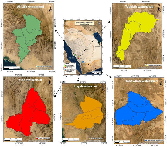
Figure 1.
Map of the basins and their subbasins at the runoff stations. Middle image is Saudi Arabia and the geographic locations of the basins, going clockwise starting from the top right image: Tabalah, Habawnah, Liyyah, Yiba, and Al-Lith Basins.
Figure 2 shows a sample of rainfall and runoff events in the study area. Most of the data regarding the basins such as basin areas, recorded events period, and date of recorded events, number of records, and peak discharge (Qp) can be found in Ewea et al. [21,22]. The figure shows the features of the hydrographs in this arid basin. It has a steep limb rise to the peak and a sudden drop with a recession limb that is also steep but can sometimes have a long tail. These features are due to the high transmission losses in the ephemeral streams, which have been indicated by some studies [23,24] as well as the water losses in the fractured rocks in the mountainous area in the upstream region of the basins [25].
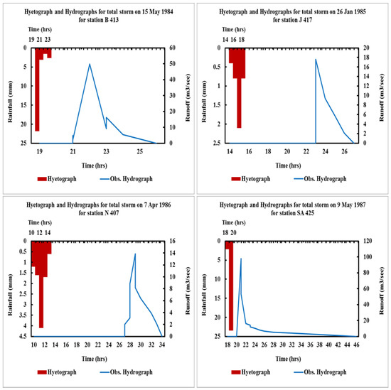
Figure 2.
Sample data of the rainfall and runoff events in the studied basins. (Top left) Hyetograph and hydrograph of the storm on 15 May 1984 for station B 413; (top right) hyetograph and hydrograph of the storm on 26 January 1985 for station J 417; (bottom left) hyetograph and hydrograph of the storm on 7 April 1986 for station N 407; (bottom right) hyetograph and hydrograph of the storm on 9 May 1987 for station SA 425.
Geologically, the Asir Cliff is part of the Arabian Shield. They are Precambrian rocks that are volcanic and metamorphic [26]. These rocks are characterized by their rigidity and resistance to erosion and absorb rainwater. The slope of the Asir Cliff is steep toward the west (Red Sea) and gradually descends toward the east (Rub al Khali). Such topography likely has a significant influence on the precipitation patterns. Wheater et al. [27] assert that annual rainfall in this area is closely related to elevation.
Examination of the rainfall data in the KSA shows that rainfall occurs in most months of the year, but with varying intensity and frequency. However, three main periods showed the highest intensity and frequency of occurrence. In winter (November/December), then in spring (April/May), and in autumn (September). Most storms are characterized by the features of convective storms: short duration, great depth, and a high degree of spatial variability. Analysis of the precipitation data shows that most thunderstorms are localized and consistent with the characteristics of thunderstorms noted by Eagleson et al. [28]. Most rainstorms lasted 1 h or less according to Wheater et al. [27,29]. In some cases, the duration of the rain increased to more than an hour and occasionally ranged from 1 to 3 h. However, in most cases, it did not exceed 4 h, except in rare cases. In Wadi Habawnah, heavier rainfall sometimes occurs (once or twice a year).
Figure 3 shows the data of the storms in the basins during the recorded period. Figure 3A is the total rainfall depth of each event in mm. Figure 3B shows the average rainfall intensity over the storm duration in mm/h. Figure 3C shows the peak discharge in m3/s, and Figure 3D shows the runoff volume in million m3. It is worth mentioning that an extreme event that produced a peak flood of 3219.65 m3/s in the Yiba Basin was omitted from the graph to visualize other data and considered as an outlier so that it did not influence the analysis. Although only 4 years of data are available for the five representative basins, a dataset of 158 was collected.
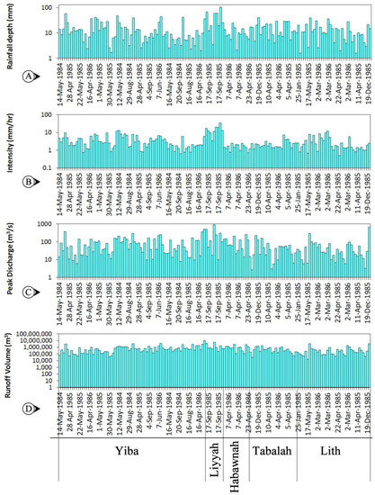
Figure 3.
Data of the storms in the basins in the recorded period: (A) rainfall depth in mm, (B) average rainfall intensity over the storm duration in mm/h, (C) peak discharge in m3/s, and (D) runoff volume in m3. Note: An extreme value of 3219.65 m3/s in the Yiba Basin was omitted from the graph to visualize other data. Note that the units of the parameters in the figure is different from the units in Table 1. This is because in the figure, they are used to present the values in the traditional way, however, in the table, they are used for the computations since they are going to transfer to logarithms.
Table 1 shows the summary statistics of the observed data of the storms required for the rational method calculations. The statistics were made in the units given in the table to be used directly in the rational method equation so that it produced the peak flow in m3/s and the runoff volume in m3, so there was no need for unit conversion.

Table 1.
Summary statistics of the observed parameters of the rational method from the storms. Note that the units of the parameters in the table is different from the units in Figure 3.
Since in the current methodology, the correlation coefficient (CC) between the parameters is required, the CC was estimated and presented in Table 1. The CC indicates weak negative correlations (CC < −0.5) for all parameters, except between the runoff coefficient and the rainfall intensity, which showed a weak positive correlation. The low correlation may be an indication of the small amount of data that we always face in arid regions. Figure 4 shows the observed relationship between the logarithms of the parameters in the rational method equation (i.e., basin area, rainfall intensity, runoff coefficient, and total storm rainfall depth). These correlations were used later in the analysis.
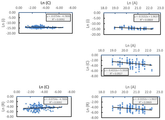
Figure 4.
The observed relationship between the logarithms of the parameters in the rational method. (Top left) Relationship between Ln (C) and Ln (i); (top right) is the relationship between Ln (A) and Ln (i); (middle) relationship between Ln (A) and Ln (C); (bottom right) is the relationship between Ln (R) and Ln (C), and (bottom right) is the relationship between Ln (A) and Ln (R).
3. Methodology
3.1. Rational Method
The rational method formula [30] reads:
where
- A = the basin area;
- C = the runoff coefficient;
- i = the intensity of the rainfall; and
- Q = the peak flood.
Al-Amri et al. [14] derived a formula for the runoff volume, V, from the peak flow of the rational method. The volume can be estimated as:
He proved that the lognormal distribution is the best to fit the variability in the rational method parameters, therefore, taking the logarithms of the equation reads:
Consequently, the runoff volume reads:
The following analysis will use the logarithm transformation of the parameters and in the end, the anti-logarithm was used to transform back to the original parameters.
3.2. Joint Probability Distribution of the Rational Method Parameters
In the current study, we considered the logarithm of the parameters of the rational method as a multi-variate normal distribution since it has been proven by Al-Amri et al. [14] that the marginal distribution of the parameters follows a lognormal distribution.
The p-variate probability density function is given by Mood and Graybill [31]:
where
- X = the p-vector of variables;
- = the vector of the mean of the variables;
- = the covariance matrix of the variables;
- p = the number of variables; and
- T = transpose operation of the matrix.
In the case of tri-variate distribution (ln(A), ln(C), and ln(i)) for the rational method of the peak flow or (ln(A), ln(C), and ln(R)) for the rational method of the runoff volume, we can use the following notations: X1 for ln(A), X2 for ln(C), and X3 for ln(i) or ln(R), depending on which equation (Equation (1) or (2)) is under study.
Therefore, we shall have:
where
- = the mean of the variable Xj and j = 1, 2, and 3;
- = the variance of the variable Xj;
- = the covariance between variables Xj and Xk where k = 1, 2, and 3.
The correlation coefficient between variables Xj and Xk is defined as:
For the tri-variate system, as in the current study, there are three correlation coefficients: ρ12 = ρ23, ρ13 = ρ31, and ρ23 = ρ32.
3.3. Uncertainty Quantification
Two uncertainty quantification methods were implemented, namely: the first-order second-moment (FOSM) and Monte Carlo Simulation (MC).
The FOSM is based on Taylor series expansion, which is truncated at the second-order term. The variance of the output variable is related to the standard deviation of the uncertain input parameters.
The FOSM was applied by Al-Amri et al. [14] to the rational method formulas for both the peak flow and runoff volume and produced the following relationships:
where
- = variance of the logarithms of the peak discharge;
- = variance of the logarithms of the runoff coefficient;
- = variance of the logarithms of the rainfall intensity;
- = variance of the logarithms of the area;
- = covariance of the logarithms of runoff coefficient and the logarithms of the rainfall intensity;
- = covariance of the logarithms of runoff coefficient and the logarithms of the area; and
- = covariance of the logarithms of the area and the logarithms of the rainfall intensity.
Additionally, the variance for the volume is expressed as:
- = variance of the logarithms of the runoff volume;
- = variance of the logarithms of the rainfall depth;
- = covariance of the logarithms of runoff coefficient and the logarithms of the rainfall depth; and
- = covariance of the logarithms of the area and the logarithms of the rainfall depth.
It can be noticed from Equations (6) and (7) that the variance in the logarithm of the discharge or the logarithm of the volume is the sum of the variance of the logarithms of the parameters C, i, R, and A and their covariances.
The probabilistic MC method is based on many random experiments. Concerning the chosen distribution, the uncertain parameters are randomized and for each realized parameter of the inputs (the rainfall intensity or depth, the basin area, and the runoff coefficient), the corresponding output variables (the peak discharge and the volume) are estimated; therefore, a set of output variables are generated. The ensemble mean, the ensemble standard deviation of the realized input parameters and the generated output variables can be estimated. Additionally, a complete statistical analysis of the model results is performed (such as the distribution percentiles, and upper and lower uncertainty bounds at 95% and 99% confidence). The number of experiments must be sufficiently large to ensure reliable results (1000 realizations are obtained).
The generation process follows the steps below [31]:
The first step is the generation of the realization of the basin area from the normal distribution, N (μ, σ), of the logarithm of the basin area from the formula:
The second step is the generation of the realization of the runoff coefficient from the normal distribution of the logarithm of the runoff coefficient from the formula:
where a and b are given by:
The third step is the generation of the realization of the rainfall intensity or rainfall depth from the normal distribution of the logarithm of the rainfall intensity or rainfall depth from the formula:
where c and d are given by:
Therefore, the generation of the peak flow and the runoff volumes are estimated by the anti-logarithms for the peak flow as:
and for the runoff volume:
Since we obtained 1000 realizations in the MC simulations, the mean, variance, and percentiles of the generated realizations in the log transformation are related to the original mean, M, variance, Var, and percentiles, Xp by:
where is the inverse of the error function and p is the percentile (0.01, 0.02, …, and 0.99).
3.4. Uncertainty Analysis
The uncertainty analysis was performed based on the probabilistic forecast technique described in the previous section. The generated realizations of the input and the predicted outputs were plotted with the data to test the consistency of the model. Data visualization as scatterplots offers the possibility to show the distribution of all random experiments to examine the behavior of the model. Additionally, quantile plots of the data and the generated realizations with the line of perfect fit showed the goodness-of-fit of the distributions of both the data and the realizations.
4. Results and Discussion
The following sections show the results of the study represented in some graphs, a summary table, and discussion of the outcomes.
4.1. Comparison between the Data and the Generated Realizations of the Rational Method Input Parameters
Figure 5 shows both the data of the parameters of the rational method and the corresponding realizations generated by the Monte Carlo method. Figure 5A is the basin area, Figure 5B is the runoff coefficient, Figure 5C is the rainfall intensity, and Figure 5D is the runoff depth. It should be mentioned that the generated realizations are not a time series; these were projected for each basin for the same event. This was meant to show the variability and it is assumed that the variability was the same over all the basins since we had a limited number of events. Additionally, the confidence interval for each parameter was plotted at both 95% and 99%. The stochastic model represents the variability reasonably well, since both the data and the generated realizations fell within the confidence limits. Even though there were some extreme data outside the confidence limits, a similar observation was noticed with the simulation, which confirms the statistical similarity between the data and the simulation.

Figure 5.
Comparison between the data and the generated realizations of the rational method input parameters with 95% and 99% confidence: (A) Basin area, (B) runoff coefficient, (C) average rainfall intensity, and (D) runoff depth.
4.2. Comparison between the Data and the Generated Realizations of the Rational Method Output Variables
Figure 6 shows a comparison between the data and the simulation of the output variables of the rational method. Figure 6A shows the peak discharge. The runoff volume is presented in Figure 6B. The confidence intervals for both the peak flow and runoff volume are also presented at the 95% and 99% confidence levels. The results show that the simulations fell within the 95% and 99% confidence levels for both Qp and V. Only limited simulations were outside the limits. This was expected since the generation process can produce some extreme events that go out of bounds. However, the majority were within the bounds.
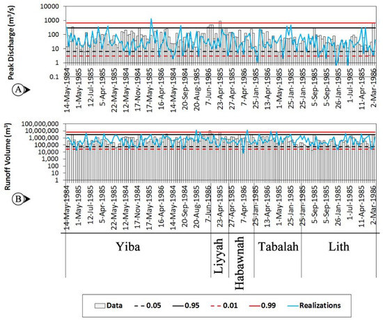
Figure 6.
Comparison between the data and the generated realizations of the rational method output variables with 95% and 99% confidence levels: (A) Peak discharge, and (B) runoff volume.
4.3. Comparison between the Correlation of the Parameters in the Rational Method and the Generated Realizations
Figure 7 shows a comparison between the correlation of the parameters of the rational method, in a log-transformation format, and the generated realizations. The blue dots are the data, and the orange dots are the generated realizations. It can be seen that both the data and simulations were pretty close to each other. Additionally, the trending lines for both data (black line) and the realizations (green line) coincided with each other with some marginal deviations and slightly different inclinations, which was due to the randomness in the generated realizations. However, they provided reasonably good results.
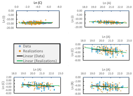
Figure 7.
Comparison between the correlation of the parameters from the data and the generated realizations in a logarithmic scale. (Top left) Relationship between Ln (C) and Ln (i); (top right) relationship between Ln (A) and Ln (i); (middle right) is the relationship between Ln (A) and Ln (C); (bottom right) relationship between Ln (R) and Ln (C); and (bottom right) relationship between Ln (A) and Ln (R).
4.4. Comparison between Probability Distributions of the Peak Flow, Runoff Volumes, and the Realizations
Figure 8 (top) shows a comparison between the probability distribution of the peak flow data, the theoretical log-normal distribution, and the probability distribution of the MC realizations generated by three estimation methods of rainfall intensity, namely: (1) the average intensity of the storms (i.e., the total rainfall divided by the rainfall duration); (2) the maximum intensity within the storm; and (3) the intensity calculated by the total rainfall of the storm divided by the time of concentration [32]:
where is in hours; is the length of the channel from headwater to the outlet in km; and is the average watershed slope.
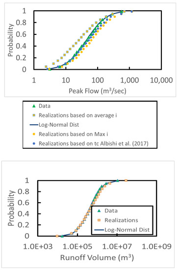
Figure 8.
Comparison between the probability distributions of the data and the realizations. (Top) Peak flow, (bottom) runoff volume. The top image shows the comparison for the peak flow with a different estimation of intensity (average intensity of the storm, maximum intensity of the storm, and intensity calculated by the time of concentration of the basin based on [32]).
The results show that the probability distribution of the peak flow data and the theoretical log-normal distribution matched well. This was confirmed by the earlier study of Al-Amri et al. [14]. The probability distribution of the MC realizations generated by the time of concentration estimated by Albishi et al. [32] also matched very well with both the data and the theoretical log-normal distribution, however, the probability distribution of the MC realizations generated by the maximum intensity within the storm showed an overestimation of the probability distribution and in contrast, the MC realizations generated by the average intensity showed an underestimation of the probability distribution. Therefore, the use of the equation of the time of concentration estimated by Albishi et al. [32] is good for simulating the peak flow in the rational methods in ungauged basins in the Saudi arid environment.
Figure 8 (bottom) shows a comparison between the probability distribution of the data of the runoff volume and the theoretical log-normal distribution and the probability distribution of the MC realizations of the runoff volume. Both the data and the MC realizations matched well with the theoretical distribution, which means that log-normal distribution can be used to generate runoff volumes in ungauged basins.
4.5. Comparison between the Quantiles of the Data and the Realizations
Figure 9 shows the quantile plots between the rational method parameters (C, i, A, and R), peak flow, runoff volume, and the corresponding generated realizations. The figure shows the quantiles of the data (on the y-axis) and the realizations (on the x-axis). Additionally, a line of perfect model fit (1:1) is presented. The figure showed good agreement between the data and the realizations for the parameters. However, one may note that some very extreme values in the realizations may occur. This is due to the tail of the long-normal distribution, since a value of a very low probability of occurrence (i.e., at the tail of the distribution) may be realized in the generation process, leading to what is sometimes called an “outlier”. However, the majority of the data fell on line 1:1. This gives confidence to the model, and therefore, the model can be used for predictions of ungauged basins that have similar characteristics to these basins.
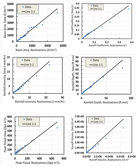
Figure 9.
Quantile plots of the data and the realizations of the rational method parameters (first row: basin area and runoff coefficient; second row: rainfall intensity and rainfall depth; and last row: peak flow, and runoff volumes).
4.6. Comparison between Statistics of the Data and the Statistics of FOSM and MC
Table 2 shows a comparison between the statistics of the data and the statistics of the FOSM and MC simulations. The table shows that the FOSM and the MC based on the average intensity underestimated the mean peak flow by 14 m3/s and 9 m3/s, respectively, however, the MC based on the time of concentration (tc) estimated by Albishi et al. [32] and the maximum intensity of the storm overestimated the mean peak flow in the data by 34 m3/s and 37 m3/s, respectively. This indicates that the use of the MC method is better than the use of FOSM for the estimation of the mean peak flow since FOSM is a linearized approach and MC is a generalized one. However, for the standard deviation (SD) of the peak flow, both FOSM and MC at various intensities overestimated the SD of the peak flow in the data. The lowest overestimation was obtained by FOSM, and the highest overestimation was obtained by MC based on the intensity estimated by the maximum intensity. Regarding the coefficient of variation (CV), the MC with intensity based on [32] had a CV = 1.6, which was closest to the CV in the data (CV = 1.4), indicating that the generated values were in good agreement with the data, although the mean of the MC overestimated the data. This was also confirmed by Figure 8 (top), where the distribution of data almost coincided with the distribution based on intensity. This led to the conclusion that the estimation of the time of concentration in these wadis by Albishi et al. [32] is appropriate for peak flow estimation. This result confirms the earlier study by Al-Amri et al. (2022) [14]. The CV of FOSM was 2.2, which provides the highest overestimation among the MC with different intensities. Therefore, it is preferable to use MC rather than FOSM. The FOSM can only produce a quick overview of the uncertainty before performing MC simulations.
Table 2.
Comparison between the statistics of the data and statistics of the FOSM and MC.
Regarding the runoff volume, the FOSM still provided an underestimation of both the mean and SD, however, the MC method proved values in almost the same range of the data. However, the CV of the FOSM (2.1) was relatively close to the CV of the data (2.4), while for MC, the CV was 1.9, which was slightly lower than the FOSM. This means that both the FOSM and MC methods provide the same order of magnitude of the CV of the data. Therefore, both of them provide an acceptable estimation from a practical point of view.
5. Summary and Conclusions
In this paper, we analyzed the rational method equation in a stochastic context in which the input parameters of the method (basin area, runoff coefficient, rainfall intensity, and rainfall depth) were treated as stochastic variables described by a joint probability distribution (tri-variate log-normal distribution) defined by the mean, variance of the input parameters, and the covariance between the input parameters or their correlation coefficient. The MC method was used to generate realizations of the input parameters, and the output variables (peak flow and runoff volume) were estimated by the rational method equations. Statistical analysis was performed between the data and the generated realizations, and the following conclusions were drawn from the study:
- The correlation coefficient between the rational method parameters (C, A, i, and R) was relatively weak; it also showed a negative correlation except between C and i. The correlation coefficient between A and i was the strongest (0.46), while that between C and R was the weakest.
- Although the correlation between the parameters was weak, the model was capable of simulating the rational model parameters and estimating the Qp and V reasonably well. The reason is that the relations for the generation process do not depend only on the correlations, but also depend on the mean and variance of the parameters.
- The log-normal distribution fit both the data and the generated peak flow well using the rainfall intensity generated from the time of concentration equation developed by some researchers in the literature. Furthermore, the log-normal distribution fit both the data and the generated runoff volumes well. Therefore, the log-normal distribution can be used as a model for the generation of the peak flow and runoff volume in ungagged basins.
- The use of the FOSM method underestimates the data in comparison with the MC method. Therefore, we recommend using the MC method with an intensity calculated with the tc equation [32], since the CV = 1.6, which was the closest to the data (CV = 1.4). However, in terms of runoff volume, FOSM and MC provided a CV = 2.1 and 1.9, respectively, which were in the order of magnitude of the CV of the data (2.4). Therefore, both methods provide an acceptable estimation from a practical point of view.
- The generated realizations fell within the confidence levels, except for a few marginal cases, which are expected due to the long tail of the log-normal distribution, and consequently, an extreme event may occur.
- The model can be used to generate peak flows and the associated confidence limits in ungagged basins from the statistics of the rainfall, basin area, and runoff coefficient based on the equations developed in this study.
Author Contributions
Conceptualization, A.M.E. and N.S.A.-A.; Methodology A.M.E. and H.A.E.; Software, A.M.E.; Validation, A.M.E., N.S.A.-A. and H.A.E.; Formal analysis, N.S.A.-A., A.M.E. and H.A.E.; Investigation, N.S.A.-A., A.M.E. and H.A.E.; Resources, A.M.E. and H.A.E.; Writing original draft preparation, A.M.E.; Writing—review and editing, A.M.E., N.S.A.-A. and H.A.E.; Visualization, A.M.E., H.A.E. and N.S.A.-A.; Project administration, N.S.A.-A. All authors have read and agreed to the published version of the manuscript.
Funding
This work was funded by the Deanship of Scientific Research (DSR), King Abdulaziz University, Jeddah, under grant no. (G-336-155-1441).
Institutional Review Board Statement
Not applicable.
Informed Consent Statement
Not applicable.
Data Availability Statement
The authors have no permission to submit the data since it belongs to the Ministry.
Acknowledgments
This work was supported by the Deanship of Scientific Research (DSR), King Abdulaziz University, Jeddah, under grant no. (G-336-155-1441). The authors, therefore, gratefully acknowledge the DSR technical and financial support.
Conflicts of Interest
The authors declare that they have no known competing financial interest or personal relationships that could have appeared to influence the work reported in this paper.
References
- Almazroui, M. Simulation of present and future climate of Saudi Arabia using a regional climate model (PRECIS). Int. J. Clim. 2013, 33, 2247–2259. [Google Scholar] [CrossRef]
- Farquharson, F.; Meigh, J.; Sutcliffe, J. Regional flood frequency analysis in arid and semi-arid areas. J. Hydrol. 1992, 138, 487–501. [Google Scholar] [CrossRef]
- Cordery, I.; Fraser, J. Theme 4-6-Some Hydrological Characteristics of the Australian Arid Zone; National Institute of Hydrology: Roorkee, India, 2000. [Google Scholar]
- Nemec, J.; Rodier, J.A. Streamflow characteristics in areas of low precipitation (with special reference to low and high flows). In The Hydrology of Areas of Low Precipitation; International Association of Hydrological Sciences: Paris, France, 1979; pp. 125–140. [Google Scholar]
- McMahon, T. Hydrological characteristics of arid zones. In The Hydrology of Areas of Low Precipitation; International Association of Hydrological Sciences: Paris, France, 1979; pp. 105–123. [Google Scholar]
- Pilgrim, D.H.; Chapman, T.G.; Doran, D.G. Problems of rainfall-runoff modelling in arid and semiarid regions. Hydrol. Sci. J. 1988, 33, 379–400. [Google Scholar] [CrossRef]
- Majone, B.; Avesani, D.; Zulian, P.; Fiori, A.; Bellin, A. Analysis of high streamflow extremes in climate change studies: How do we calibrate hydrological models? Hydrol. Earth Syst. Sci. 2022, 26, 3863–3883. [Google Scholar] [CrossRef]
- Bedient, P.B.; Huber, W.; Vieux, B. Hydrology and Floodplain Analysis; Pearson: New York, NY, USA, 2008; Volume 816. [Google Scholar]
- Hua, J.; Liang, Z.; Yu, Z. A modified rational formula for flood design in small basins 1. JAWRA J. Am. Water Resour. Assoc. 2003, 39, 1017–1025. [Google Scholar] [CrossRef]
- Wang, S.; Wang, H. Extending the Rational Method for assessing and developing sustainable urban drainage systems. Water Res. 2018, 144, 112–125. [Google Scholar] [CrossRef]
- Pilgrim, D.; Cordery, I. Flood runoff. In Handbook of Hydrology; Chapter 9; Maidment, D., Ed.; McGraw-Hill, Inc.: New York, NY, USA, 1993. [Google Scholar]
- Titmarsh, G.W.; Cordery, I.; Pilgrim, D.H. Calibration Procedures for Rational and USSCS Design Flood Methods. J. Hydraul. Eng. 1995, 121, 61–70. [Google Scholar] [CrossRef]
- Chin, D.A. Estimating Peak Runoff Rates Using the Rational Method. J. Irrig. Drain. Eng. 2019, 145, 04019006. [Google Scholar] [CrossRef]
- Al-Amri, N.S.; Ewea, H.A.; Elfeki, A.M. Revisit the rational method for flood estimation in the Saudi arid environment. Arab. J. Geosci. 2022, 15, 532. [Google Scholar] [CrossRef]
- Dhakal, N.; Fang, X.; Cleveland, T.G.; Thompson, D.B. Revisiting modified rational method. In World Environmental and Water Resources Congress 2011: Bearing Knowledge for Sustainability; American Society of Civil Engineers: Reston, WV, USA, 2011; pp. 751–762. [Google Scholar]
- Young, C.B.; McEnroe, B.M.; Rome, A.C. Empirical Determination of Rational Method Runoff Coefficients. J. Hydrol. Eng. 2009, 14, 1283–1289. [Google Scholar] [CrossRef]
- Efstratiadis, A.; Koussis, A.D.; Koutsoyiannis, D.; Mamassis, N. Flood design recipes vs. reality: Can predictions for ungauged basins be trusted? Nat. Hazards Earth Syst. Sci. 2014, 14, 1417–1428. [Google Scholar] [CrossRef]
- Kottek, M.; Grieser, J.; Beck, C.; Rudolf, B.; Rubel, F. World map of the Köppen-Geiger climate classification updated. Meteorol. Z. 2006, 15, 259–263. [Google Scholar] [CrossRef] [PubMed]
- Sharon, D. The spottiness of rainfall in a desert area. J. Hydrol. 1972, 17, 161–175. [Google Scholar] [CrossRef]
- Dames, M. Representative Basins Study for Wadi: Yiba, Habwnah, Tabalah, Liyyah and Al-Lith (Main Report) Kingdom of Saudi Arabia, Ministry of Agriculture and Water; Water Resource Development Department: Riyadh, Saudi Arabia, 1988. [Google Scholar]
- Ewea, H.A.; Elfeki, A.; Al-Amri, N. Development of intensity–duration–frequency curves for the Kingdom of Saudi Arabia. Geomat. Nat. Hazards Risk 2017, 8, 570–584. [Google Scholar] [CrossRef]
- Ewea, H.A.; Al-Amri, N.S.; Elfeki, A.M. Analysis of maximum flood records in the arid environment of Saudi Arabia. Geomat. Nat. Hazards Risk 2020, 11, 1743–1759. [Google Scholar] [CrossRef]
- Abdulrazzak, M.J.; Sorman, A.U. Transmission Losses from Ephemeral Stream in Arid Region. J. Irrig. Drain. Eng. 1994, 120, 669–675. [Google Scholar] [CrossRef]
- Elfeki, A.M.M.; Ewea, H.A.R.; Bahrawi, J.A.; Al-Amri, N.S. Incorporating transmission losses in flash flood routing in ephemeral streams by using the three-parameter Muskingum method. Arab. J. Geosci. 2015, 8, 5153–5165. [Google Scholar] [CrossRef]
- Farran, M.M.; Elfeki, A.; Elhag, M.; Chaabani, A. A comparative study of the estimation methods for NRCS curve number of natural arid basins and the impact on flash flood predications. Arab. J. Geosci. 2021, 14, 121. [Google Scholar] [CrossRef]
- Al-Shanti, A.; El-Mahdy, O.; Hassan, M.; Hussein, A. A Comparative Study of Five Volcanic-Hosted Sulfide Mineralizations in the Arabian Shield. Earth Sci. 1993, 6, 1–33. [Google Scholar] [CrossRef]
- Wheater, H.; Butler, A.; Stewart, E.; Hamilton, G. A multivariate spatial-temporal model of rainfall in southwest Saudi Arabia. I. Spatial rainfall characteristics and model formulation. J. Hydrol. 1991, 125, 175–199. [Google Scholar] [CrossRef]
- Eagleson, P.S.; Fennessey, N.M.; Qinliang, W.; Rodriguez-Iturbe, I. Application of spatial Poisson models to air mass thunderstorm rainfall. J. Geophys. Res. Atmos. 1987, 92, 9661. [Google Scholar] [CrossRef]
- Wheater, H.; Onof, C.; Butler, A.; Hamilton, G. A multivariate spatial-temporal model of rainfall in southwest Saudi Arabia. II. Regional analysis and long-term performance. J. Hydrol. 1991, 125, 201–220. [Google Scholar] [CrossRef]
- Chow, V.; Maidment, D.; Mays, L. Applied Hydrology; International Editions; McGraw-Hill: New York, NY, USA, 1988. [Google Scholar]
- Mood, A.M. Introduction to the Theory of Statistics; McGraw-Hill: New York, NY, USA, 1950. [Google Scholar]
- Albishi, M.; Bahrawi, J.; Elfeki, A. Empirical equations for flood analysis in arid zones: The Ari-Zo model. Arab. J. Geosci. 2017, 10, 51. [Google Scholar] [CrossRef]


Disclaimer/Publisher’s Note: The statements, opinions and data contained in all publications are solely those of the individual author(s) and contributor(s) and not of MDPI and/or the editor(s). MDPI and/or the editor(s) disclaim responsibility for any injury to people or property resulting from any ideas, methods, instructions or products referred to in the content. |
© 2023 by the authors. Licensee MDPI, Basel, Switzerland. This article is an open access article distributed under the terms and conditions of the Creative Commons Attribution (CC BY) license (https://creativecommons.org/licenses/by/4.0/).