Optimal Model Predictive Control for Virtual Inertia Control of Autonomous Microgrids

Abstract

For the time being, renewable energy source (RES) penetration has significantly increased in power networks, particularly in microgrids. The overall system inertia is dramatically decreased by replacing traditional synchronous machines with RES. This negatively affects the microgrid dynamics under uncertainties, lowering the microgrid frequency stability, specifically in the islanded mode of operation. Therefore, this work aims to enhance the islanded microgrid frequency resilience using the virtual inertia frequency control concept. Additionally, optimal model predictive control (MPC) is employed in the virtual inertial control model. The optimum design of the MPC is attained using an optimization algorithm, the African Vultures Optimization Algorithm (AVOA). To certify the efficacy of the proposed controller, the AVOA-based MPC is compared with a conventional proportional–integral (PI) controller that is optimally designed using various optimization techniques. The actual data of RES is utilized, and a random load power pattern is applied to achieve practical simulation outcomes. Additionally, the microgrid paradigm contains battery energy storage (BES) units for enhancing the islanded microgrid transient stability. The simulation findings show the effectiveness of AVOA-based MPC in improving the microgrid frequency resilience. Furthermore, the results secure the role of BES in improving transient responses in the time domain simulations. The simulation outcomes are obtained using MATLAB software.

1. Introduction

Integrating RES into electric grids is gaining more interest for generating electric power since it is considered a great solution for overcoming the environmental issues and problems of energy shortage [1]. Thus, RES is a significant part of small energy systems, which are microgrids. A microgrid is identified as a small power system in which RES, small generating power plants, power storage elements, residential, and industrial loads are connected [2,3]. Nevertheless, RES is connected to microgrids through power electronic converters for power exchange. Therefore, the microgrid dynamic stability is negatively affected due to the decrease in microgrid inertia provoked by power electronic converters’ interface-based RES [4,5]. Thus, the high-level utilization of RES in microgrids lowers the overall grid inertia compared to conventional synchronous generating units [6]. Furthermore, regarding the operation of the microgrids, a microgrid may operate in one of two modes: grid-connected or islanded mode of operation [7,8,9]. In islanded operation, power is not exchanged between the islanded microgrid and the grid power network [10,11]. This makes islanded microgrid frequency control more challenging, especially in uncertainties, such as the high-level deployment of RES [12,13].

To overcome the drawback driven by the reduction in the microgrid inertia, a frequency control model depends on emulating the inertia behavior produced by synchronous generators, thus enhancing the microgrid frequency resilience [14]. This control concept is a virtual synchronous machine or generator (VSG, VSG) [15]. A VSG is provided to imitate the physical characteristics of conventional synchronous generators virtually to increase the overall microgrid inertia leading to enhancement in the transient stability of the system frequency [16]. The concept of virtual inertial control is regarded as a particular portion of VSM implementation that depends on mimicking prime move properties to deliver the inertial power needed by microgrids for frequency stability support [17]. The proposed control strategy supplies the microgrid with the necessary active power through energy storage systems (ESS) and inverters by measuring the rate of frequency change (RFC) and hence reduces the microgrid frequency fluctuations during the system transients [18].

In recent years, various control strategies have been developed for dealing with the high penetration of RES into the virtual inertial control loop for frequency stability enhancement [19,20,21,22,23,24]. In [19,20], a virtual inertia control model with an enhanced strategy based on a derivative technique was utilized to provide the damping and inertial characteristics to enhance the microgrid frequency resilience. In [21], fuzzy logic control was implemented with virtual inertial control to adjust the virtual inertial gain based on the system input signals, RES penetration level, and load disturbances. In [22], a control strategy based on the coefficient diagram method (CDM) was developed in the virtual inertia model to alleviate the frequency fluctuations during high-RES integration in an islanded microgrid. In [23], the H-infinite control method was introduced into the virtual inertia model for the frequency enhancement of the islanded microgrid dynamic performance against contingencies. Furthermore, in [24], an optimal CDM was developed with the virtual inertial control to improve the dynamic performance of a two-area interconnected microgrid, including RES penetration and electric vehicles (EV). Despite the decent dynamic performance of the aforementioned control strategies [21,22,23,24], they suffer from drawbacks such as long computational time, reliance on the control designer’s experience, and the need for order reduction. In [25,26], a virtual inertia control model based on superconducting magnetic energy storage (SMES) technology was implemented to support low-inertia microgrids. In [27,28], a conventional PI controller was implemented in an islanded microgrid’s virtual inertial dynamic model to obtain the optimum controller parameters for microgrid frequency stability enhancement. Although PI controllers in [27,28] provided decent performance considering the frequency stability issues in microgrids, they have some drawbacks, such as sensitivity to controller gains, low performance to handle strong non-linearities, and sluggish response to abrupt disruptions [29].

On the other hand, the model predictive control (MPC) offers the best performance against system uncertainties and load disturbances, such as high robustness, quick response based on predictions, and fast optimization. MPC is a robust advanced control approach that depends on calculating the optimum control input signals to drive the expected outputs to the reference subjected to the system constraints. It can control systems with numerous inputs and outputs that may interact with each other [30]. MPC has been extensively used in the processing, automotive, and aerospace industries [31,32]. Furthermore, MPC can be applied to the frequency and voltage regulation of islanded and interconnected microgrids [33,34]. In [35], MPC was applied to regulate the islanded microgrid frequency considering EV and ESS. In [36], robust MPC was utilized in a two-area interconnected power system’s load frequency control (LFC). In [37], a virtual-inertia-control-based MPC was developed for the frequency control support of an isolated microgrid considering wind energy variations and load fluctuations. On the other hand, the previously mentioned works did not consider the optimal selection of MPC parameters depending on the microgrid parameters, system uncertainties, and random load fluctuations for the frequency stabilization during contingencies. According to the previous observations, this work proposes an optimal MPC-based virtual inertial control of an isolated microgrid. The optimal design of the MPC is attained using an optimization technique, the African Vultures Optimization Algorithm (AVOA). The AVOA is a recent metaheuristic technique motivated by the foraging and navigation behavior of African vultures [38]. This algorithm is easy to execute and offers excellent capability for numerous applications in many engineering design disciplines [39,40].

This article introduces an application of AVOA to obtain the MPC’s optimal design in an islanded microgrid’s virtual inertial control loop, including RES and load fluctuations. Real system uncertainties and random load fluctuations are implemented to check the microgrid performance under various scenarios. To ensure real uncertainties, actual wind power patterns are utilized and extracted from Al-Zaafrana wind power plant in Egypt, real solar power patterns are implemented from field tests, and random load fluctuations are applied. The criterion of integral square error (ISE) is utilized to define the optimization problem for the optimum design of MPC [28]. The effectiveness of the AVOA-based MPC is investigated by making a comparison to optimal conventional PI controllers that are optimally designed using various optimization algorithms, such as particle swarm optimization (PSO), genetic algorithm (GA), and manta ray foraging optimization (MRFO) algorithm [27]. Moreover, BES systems are introduced to show the considerable role of the energy storage units in improving the frequency transient stability of isolated microgrids. MATLAB software checks the suggested controller performance through real-time domain simulations.

The rest of the article is arranged as follows: Section 2 demonstrates the islanded microgrid paradigm and structure with the virtual inertia control. Section 3 presents the optimal MPC-based virtual inertia control, including formulating the optimization problem. Section 4 introduces the AVOA. The time-domain simulation outcomes are presented and discussed in Section 5. Lastly, the paper is summarized in Section 6.

2. System Modeling

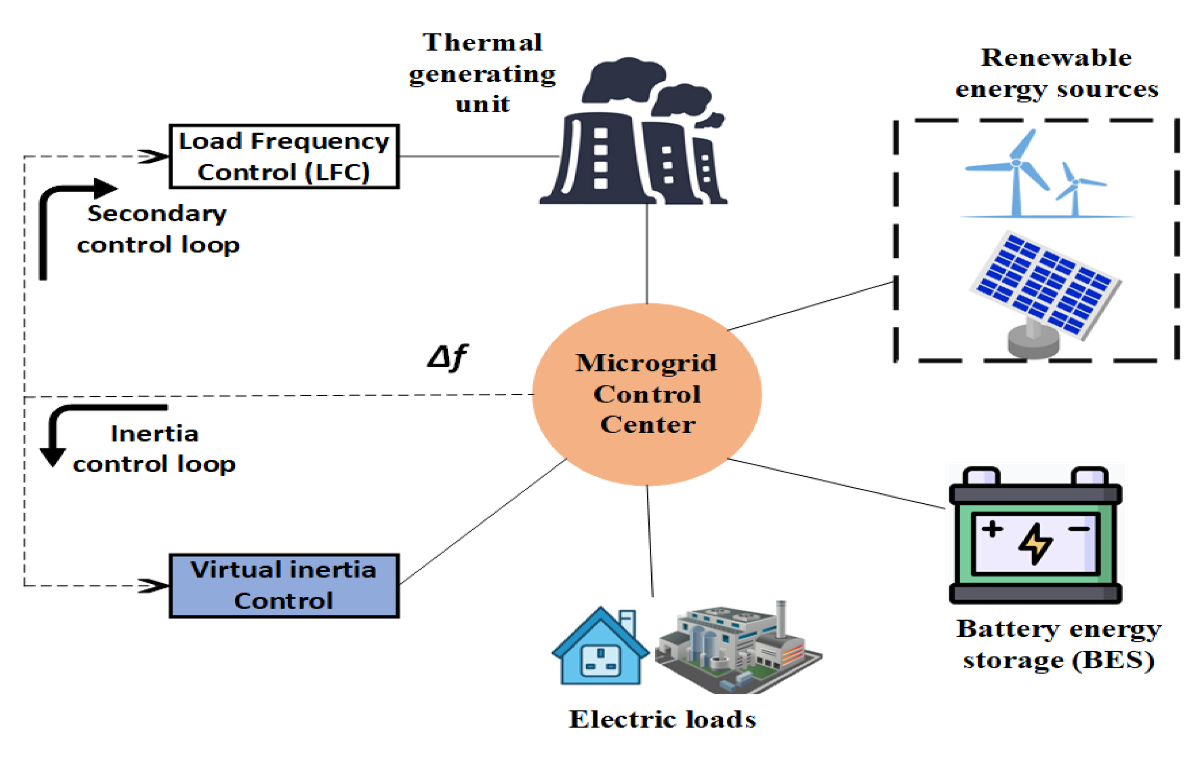
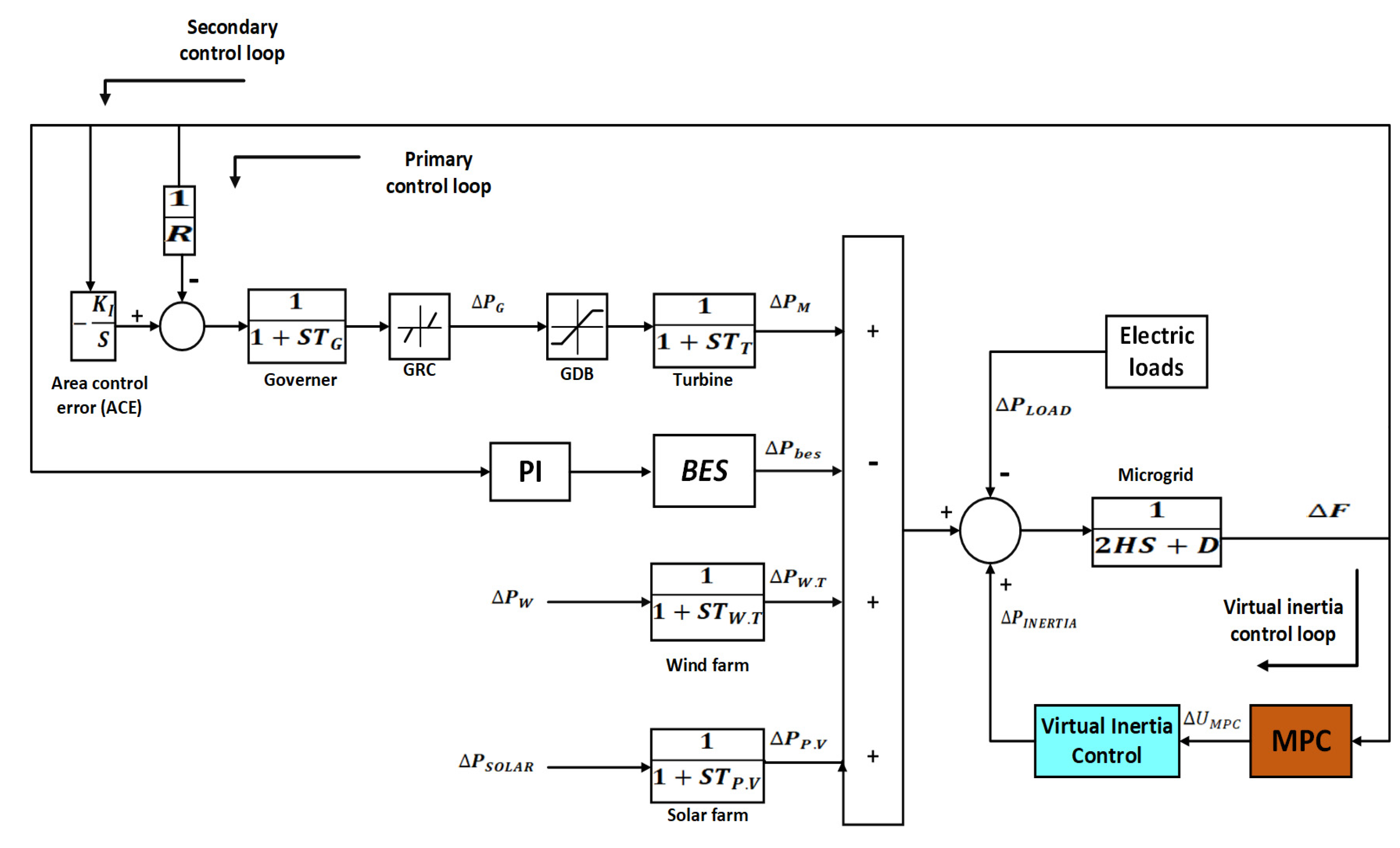
2.1. Microgrid Structure

The studied microgrid system utilized in this article is depicted in Figure 1. The islanded microgrid includes a non-reheat small thermal power station; energy storage units; electric loads with RES penetration, such as wind and PV farms; electric loads with RES penetration, such as wind; and PV farm penetration such as wind and PV farms.

For frequency control analysis, the dynamic paradigm of the investigated microgrid is depicted in Figure 2. This figure demonstrates the proposed optimal MPC in the loop of the virtual inertial control, including RES penetration (solar and wind farms), conventional thermal power unit, domestic loads, and BES units. Additionally, Figure 2 presents the modeling of the primary and secondary frequency control loops in the microgrid paradigm. Replacing many conventional synchronous generators in the microgrid with high levels of RES leads to a significant decrease in the rotating masses that are considered the main source of inertia in microgrids. Therefore, the overall system inertia is notably reduced due to the high integration of RES into the microgrid, leading to frequency stabilization issues. Thus, the primary control and load frequency control are insufficient to lessen the mismatch between the generated and demand power during contingencies [41]. Therefore, virtual inertia control is introduced to compensate for the active power mismatch and the frequency control areas. The disturbances to the microgrid system are solar/wind power and load power demand. These works use the first-order transfer functions of RES. Based on articles [23,28], it is assumed that the low-order dynamic model of RES is adequate for frequency control analysis. This work considers the essential inherent requirements and significant thermal and mechanical constraints enjoined by the dynamic actions of the thermal power unit to obtain an actual perception of the microgrid paradigm. The power generation change rate is an essential dynamic constraint of conventional thermal power units due to thermal and mechanical limitations. Two physical constraints of the thermal power unit are imposed in this paper. The first is the generation rate constraint (GRC) of conventional generating units, which is specified as 20% per minute [42]. The second constraint is the maximum/minimum values (Vu, Vl) of the steam turbine governor dead band (GDB), which are specified as 0.3 and −0.3 p.u, respectively. Furthermore, focusing on the studied microgrid dynamics, the control equations of the microgrid components are presented as follows [23,28]:

$$\Delta P_M=\frac{1}{1+S{T}_T}\Delta P_G$$

(1)

$$\Delta P_G=\frac{1}{1+S{T}_G}\left(\Delta P_C-\frac{1}{R}\Delta F\right)$$

(2)

$$\Delta P_C=\frac{K_I}{S}\Delta F$$

(3)

$$\Delta P_{W.T}=\frac{1}{1+S{T}_{W.T}}\Delta P_W$$

(4)

$$\Delta P_{P.V}=\frac{1}{1+S{T}_{P.V}}\Delta P_{SOLAR}$$

(5)

where $\Delta P_M$ is the deviation in the thermal generating unit power, $\Delta P_G$ is the deviation in the generated power from the governor unit of the thermal generating station, $\Delta P_C$ represents the deviation in the control signal of the secondary control, $\Delta F$ is the microgrid frequency deviation, $\Delta P_{W.T}$ is the deviation in the wind power plant’s active power, $\Delta P_{P.V}$ is the real generated power deviation from the solar power plant, $\Delta P_W$ represents wind power change, and $\Delta P_{SOLAR}$ is the solar power change. Furthermore, the deviation in the microgrid frequency with the effect of the primary control and secondary frequency control, as well as the inertial control loop, can be obtained as:

$$\Delta F=\frac{1}{2HS+D}\left(\Delta P_M+\Delta P_{W.T}+\Delta P_{P.V}+\Delta P_{INERTIA}-\Delta P_{LOAD}\right)$$

(6)

where $\Delta P_{INERTIA}$ is the inertial power change and $\Delta P_{LOAD}$ is the load power variation.

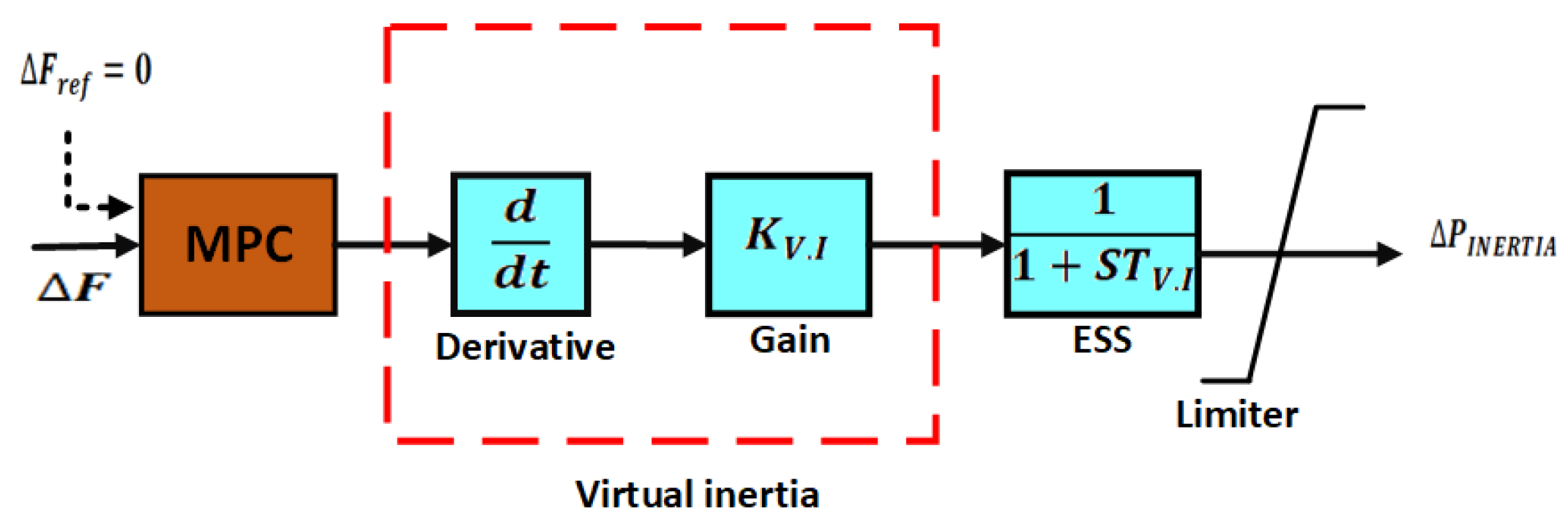
2.2. Virtual Inertia Control Modeling

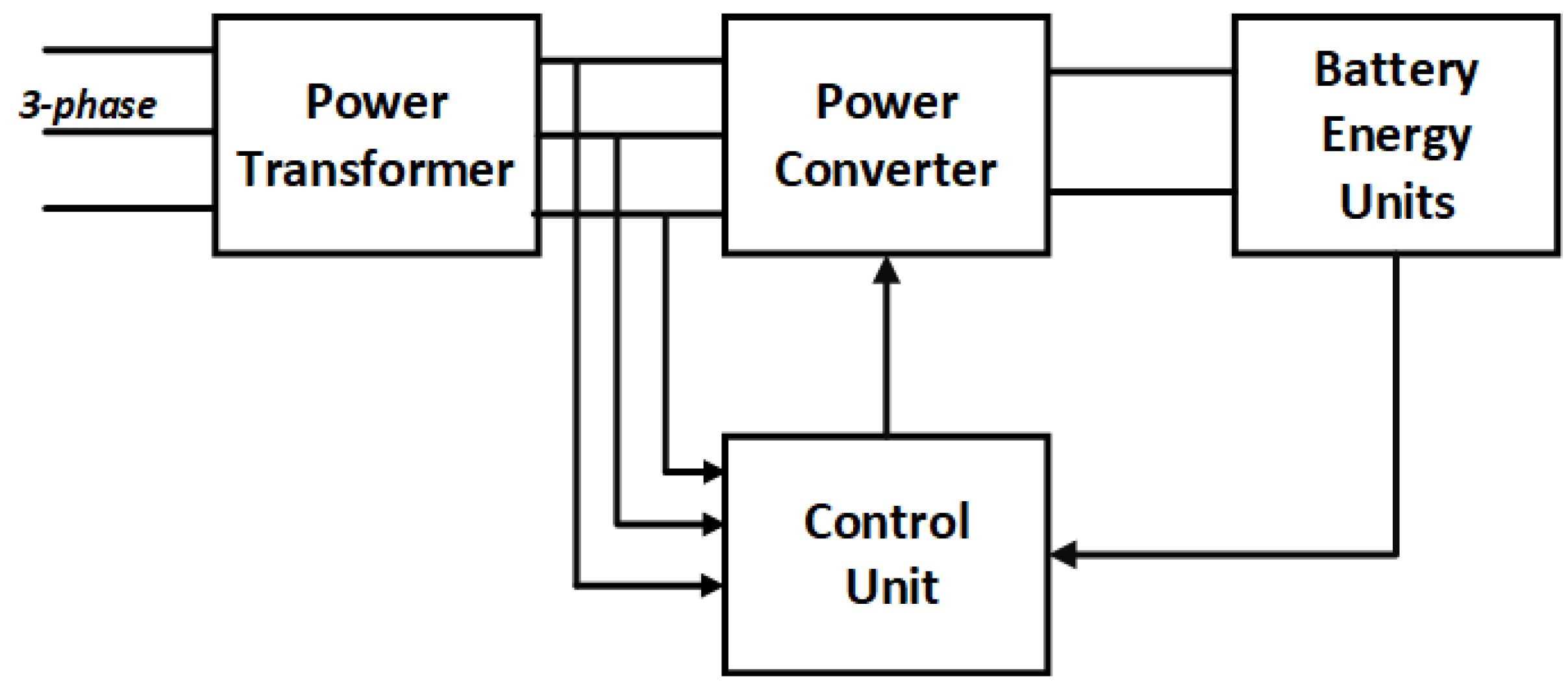
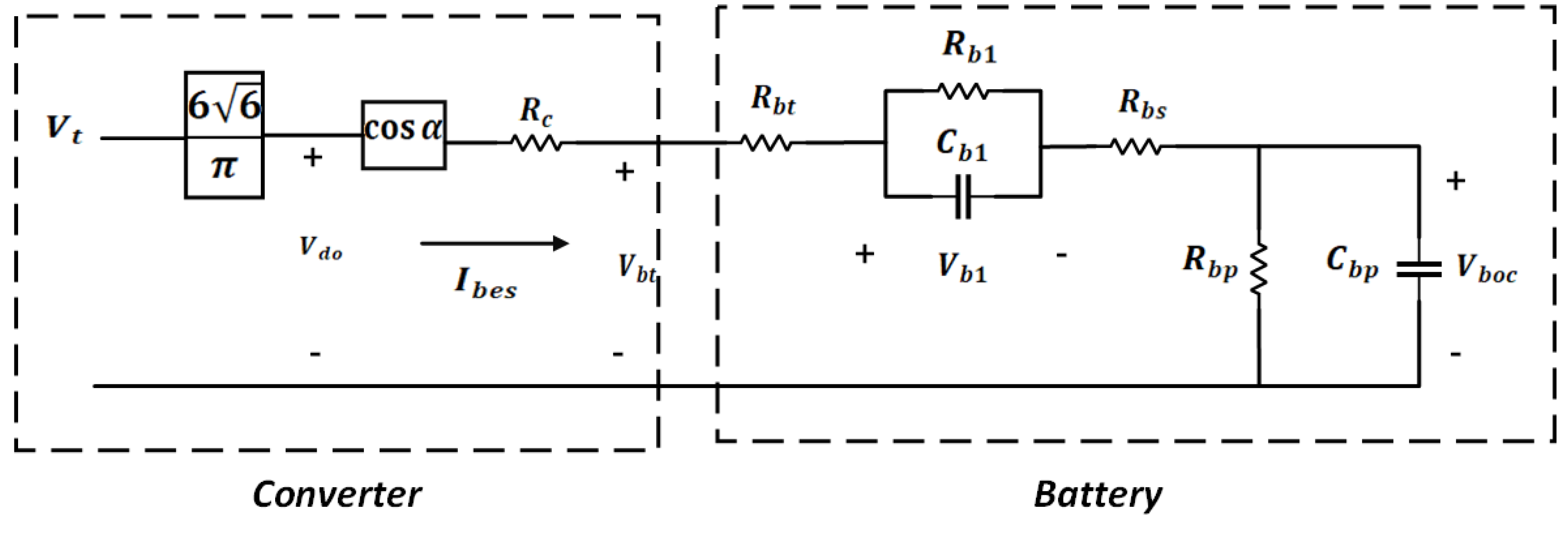
This study employs three frequency-regulating methods (i.e., inertia control, primary and secondary control processes) to maintain desirable frequency stability during high-RES penetration. During the inertial control process, the stabilization of the system frequency is achieved only due to the kinetic energy stored in the rotating masses of traditional generators or the virtual inertial control model since the primary and secondary controls have not been activated yet. The microgrid frequency is settled to a new steady state value during the primary control after the contingency. During secondary control, the steady-state error in the network frequency is eliminated by the area control error (ACE) [43]. Virtual inertia control concept is considered a particular case of VSG operation in which the action of the prime mover is imitated to provide the inertia power for the support of frequency stability [17]. Virtual inertia control is provided to connect energy storage systems (ESS) with the grid through power inverters to enable the ESS to act as a conventional generator providing damping and inertia properties of conventional generators to the system. Therefore, the virtual inertial control modeling can provide the necessary inertial power to the microgrid during the absence of conventional generators with high-RES integration. A virtual inertial control block consists of ESS, a derivative part, inertial gain, and an active power limiter, as presented in Figure 3. The virtual inertia control concept depends on calculating the rate of frequency change (RFC) using the derivative part, which is an essential element in the virtual inertia control modeling. The RFC can be calculated as follows:

$$RFC=\left[ \frac{d}{dt}\left(\Delta F\right) \right]$$

(7)

ESS is to provide adequate inertial power to the microgrid based on the RFC through inverters to reduce the unbalance in power between the generation and consumption in case of disturbances. According to references [23,28], the first-order transfer function adequately represents ESS in the virtual inertial control loop. To achieve a realistic depiction of ESS, a power limiter is provided to represent the ESS capacity with minimum and maximum values of ESS active power. Therefore, the virtual inertial control modeling represented in Figure 3 can finally provide the inertia properties of the studied microgrid for frequency regulation during high-RES penetration and system uncertainties. The imitation of the virtual inertial power can be obtained using the dynamic equation represented as follows:

$$\Delta P_{INERTIA}=\frac{K_{V.I}}{1+S{T}_{V.I}}\left[\frac{d}{dt}\left(\Delta F\right)\right]$$

(8)

where $T_{V.I}$ is the time-constant-based virtual inertia for imitating the dynamics of the ESS and $K_{V.I}$ is the virtual inertial control gain in the microgrid.

2.3. BES Modeling

The increasing integration of RES into electric networks leads to high-frequency fluctuations affecting the system frequency resilience because of the inconsistent nature of RES. Therefore, energy storage units gain great attention in enhancing the network frequency regulation and stabilizing the frequency disturbances during RES penetration and load fluctuations. The BES system is one of the most efficient energy storage units used to smooth the frequency fluctuations during disturbances, particularly in islanded microgrids. Through the use of an inverter, the BES units can produce an output of AC voltage that is stable and controllable and that has the technical benefits of a reliable power source. Additionally, it aids in the microgrid’s quick black start and keeps loads’ power supplies intact. This process mainly depends on the bidirectional active power flow between the microgrid and the BES system. The BES system has been investigated in numerous previous studies dealing with frequency control concerns owing to its importance as a frequency stabilizer [44,45]. Figure 4 shows the BES system’s typical structure, including the power transformer, power converter, control scheme, and battery modules.

According to the BES system structure, the maximum DC output voltage from the power converter is expressed as follows:

$$V_{do}=\frac{6\sqrt{6}}{\pi } V_t$$

(9)

where $V_t$ is the phase input voltage of the system. Figure 5 shows the equivalent circuit model of the BES system that consists of a converter circuit connected to a battery circuit. The input voltage to the battery circuit is calculated as follows:

$$V_{bt}=V_{do }cos\left(\alpha \right)-I_{bes }{R}_{c }=\frac{3\sqrt{6}}{\pi }{V}_t\left(cos{\alpha }_1-cos{\alpha }_2\right)-\frac{6}{\pi }{X}_{co} I_{bes}$$

(10)

where $V_{do }$ is the maximum DC voltage of the battery; ${\alpha }_1,{\alpha }_2$are the firing angles of the power converter; $I_{bes }$ is the battery flowing current; and $X_{co}$ is the commutation reactance. From the equivalent circuit model of the BES system, the following equations are obtained [46]:

$$I_{bes}=\frac{V_{bt}-V_{boc}-V_{b1}}{R_{bs}+R_{bt}}$$

(11)

$$V_{boc}=\frac{R_{bp}}{1+S{T}_{bp}} I_{bes}$$

(12)

$$V_{b1}=\frac{R_{b1}}{1+S{T}_{b1}} I_{bes}$$

(13)

$$T_{bp}=R_{bp}{C}_{bp}$$

(14)

$$T_{b1}=R_{b1}{C}_{b1}$$

(15)

where $V_{boc}$ is the open circuit voltage of the battery, $V_{b1}$ is the battery over voltage, $R_{bs}$ is battery internal resistance, $R_{bt}$ is connecting resistance, $R_{bp}$ is self-discharge resistance, $C_{bp}$ is the battery capacitance, $R_{b1}$ is the overvoltage resistance, and $C_{b1}$ is the overvoltage capacitance [47]. Based on the converter’s operation, the active and reactive power consumed or delivered by the BES system are:

$$P_{bes}=\frac{3\sqrt{6}}{\pi }{V}_t{I}_{bes}\left(cos{\alpha }_1-cos{\alpha }_2\right)$$

(16)

$$Q_{bes}=\frac{3\sqrt{6}}{\pi }{V}_t{I}_{bes}\left(sin{\alpha }_1-sin{\alpha }_2\right)$$

(17)

Only the p-modulation control approach is considered in this work since the virtual inertia control concerns only the frequency control issues. Therefore, for active power modulation, the condition of (${\alpha }_1=-{\alpha }_2=\alpha$) is applied. Therefore,

$$P_{bes}=\frac{6\sqrt{6}}{\pi }{V}_t{I}_{bes}cos\left(\alpha \right)=V_{do}{I}_{bes}cos\left(\alpha \right)$$

(18)

$$Q_{bes}=0$$

(19)

Figure 6 shows the incremental model of the BES system [44]. Based on the BES incremental model, the incremental active power can be obtained as follows:

$$\Delta P_{bes}=I_{bes}^o\Delta V_d$$

(20)

where $I_{bes}^o\Delta V_d$ is the response to system disturbances. $\Delta V_d$ is the damping signal, and it can be obtained as follows:

$$\Delta V_d=\frac{K_{bes}}{1+S{T}_{bes}}\Delta U_c$$

(21)

where $K_{bes}$ is the amplification factor, $T_{bes}$ is the time constant of the measurement device, and $\Delta U_c$ is the dispatched frequency control signal to provide the damping signal. In this work, 8 MW capacity of the BES system is connected to the microgrid. BES system includes two units (4 MW/15 MWH) that are connected in parallel. The parameters of BES systems are used and extracted from [47,48].

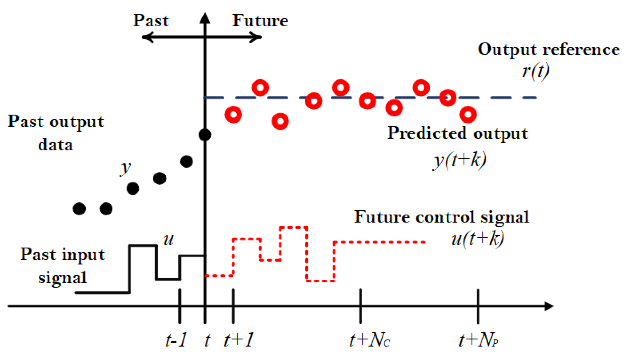
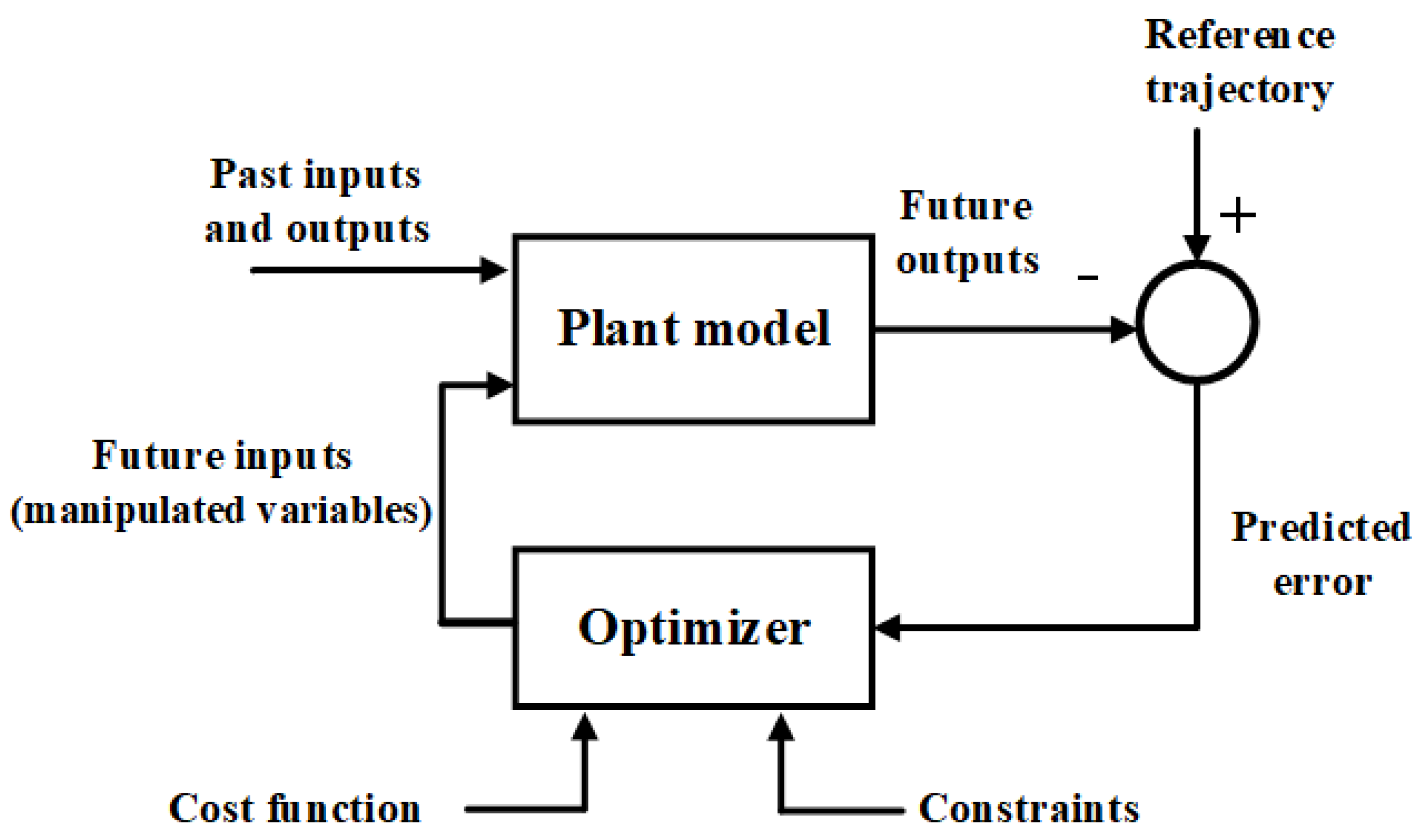
3. Optimal MPC Design

MPC has proven high performance in numerous engineering control applications, such as processing industries, automotive industries, electromechanical systems control, and many other control applications, including power system control [33,48]. Moreover, MPC has the flexibility to be applied with modern control systems, such as fuzzy logic systems, deep learning prediction models, and artificial neural networks, to work with nonlinear models [49,50]. The main target of any controller is to calculate the suitable input signal to the system such that the system output follows the desired reference. The MPC control approach relies on the explicit use of the plant model to make predictions about the future system output behavior. Furthermore, it also uses an optimizer to compute an optimum sequence of control actions to ensure that the predicted system output tracks the desired reference. Figure 7 presents the general strategy of MPC. $N_P$ is the prediction horizon, which indicates the number of future outputs predicted at each sampling instant $t$. The set of predicted outputs is $\left[\widetilde{y }\left(t+k\right), k=1,2,\dots , N_P\right]$, where $\widetilde{y }$ is the future output and $y$ is the actual system output. At the sampling time $t$, MPC computes a set of $N_C$ values of the control inputs as $\left[u\left(t+k-1\right), k=1,2,\dots , N_C\right]$, where $u$ is the manipulated input and $N_C$ is the control horizon. The set includes the present control input $u\left(t\right)$, and $N_C-1$ future control signals. The control input signals are determined to drive the predicted system outputs to the setpoint [51]. Although a set of $N_C$ input control signals is specified at each sampling instant t, the first control signal of this set is only applied to the system model. A new set of control inputs is calculated at the next sampling instant, as new state measurements are available again using the receding horizon strategy. At the next sampling instant, $y\left(t+1\right)$ is already known, all the control signals are brought up to date, and the process is repeated at the next time step [37].

Figure 8 shows the basic structure that presents the implementation of the MPC strategy. The future output of the model is predicted by utilizing the dynamic system model based on past inputs, outputs, current state, and the optimal future control inputs. By solving an online optimization problem with constraints, the control actions of the system are determined to minimize the cost function. MPC predictions are developed using the dynamic model, which is known as a linear empirical model, that is considered a multivariable form of the step response [51]. For a linear system, the following equations are used to describe the dynamics of the system:

$$x\left(t+1\right)=Ax\left(t\right)+B\left(t\right)$$

(22)

$$y\left(t\right)=Cx\left(t\right)$$

(23)

where $A, B$, and $C$ are state space matrices that describe the system model. The state output $y\left(t\right)$ usually coincides with the state $x\left(t\right)$ in microgrids. The step response model for the plant in single input single output (SISO) system is:

$$y\left(t\right)={{\displaystyle \sum }}_{i=1}^{\infty }{g}_i\Delta u\left(t-i\right)$$

(24)

where $g_i$ is the step response matrix coefficient [51]. The predicted system output is calculated as follows:

$$\widetilde{y }\left(t+k\right)={{\displaystyle \sum }}_{i=1}^{\infty }{g}_i\Delta u\left(t+k-i\right)+x\left(t+k\right)$$

(25)

where $k=\left(1,2,\dots , N_P\right)$. The predicted system outputs can be calculated for a constant disturbance as follows:

$$\widetilde{y }\left(t+k\right)={{\displaystyle \sum }}_{i=1}^k{g}_i\Delta u\left(t+k-i\right)+f\left(t+k\right)$$

(26)

where $f\left(t+k\right)$ is the free response disturbance that does not depend on the future control signals. When the dynamic model exists, it can be incorporated into the minimization process’s cost function. Several MPC techniques use various cost functions for the optimization process. The main target of MPC is to make future output $y(t$) track a specified reference signal $r\left(t\right)$ along the prediction horizon while penalizing the input control effort $\Delta u\left(t\right)$ for doing so [52]. In this paper, the weighted squared sum of the predicted errors and control input increments represent the objective function of the online optimization problem. In a single-input, single-output (SISO) system, the cost function is expressed as follows:

$$J={{\displaystyle \sum }}_{k=1}^{ N_P}{W}_y{\left[\widetilde{y }\left(t+k\right)-r\left(t+k\right)\right]}^2+{{\displaystyle \sum }}_{k=1}^{ N_C}{W}_U{\left[ \Delta u\left(t+k-1\right)\right]}^2$$

(27)

subjected to the following constraints:

$$\Delta \ge \Delta u\ge \Delta u_{min}$$

$$y_{max}\ge y\ge y_{min}$$

where $W_y$ and $W_U$ are parameters that consider the relative weight of errors on the system output and control input. The weight parameters may be constants or exponential sequences. This work assumes that the weight parameters are constant [37].

In this work, MPC is added to the virtual inertial control loop to provide the optimum input sequence $\Delta u_{MPC}$ to the virtual inertial block during high-RES penetration and load fluctuations, as presented in Figure 2. Furthermore, the virtual inertial model provides the proper amount of inertia power, $\Delta P_{INERTIA}$, to the studied microgrid so that the microgrid frequency deviation tracks the zero-frequency reference to stabilize the frequency fluctuations during disturbances while accepting the given constraints over the output frequency deviation and the inertia power change. The following steps describe the main MPC algorithm, from obtaining the basic data to applying the final control signal:

• Step 1: At sampling instant $t$, MPC measures the microgrid output frequency change $\Delta f\left(t\right)$.
• Step 2: Based on the current microgrid frequency information, MPC computes sequence of control actions $\Delta U_{MPC}\left(t+k-1\right), k=1,2,\dots , N_C.$
• Step 3: Only the first control step $\Delta U_{MPC}\left(t\right)$ is applied to the virtual inertia model to obtain the injected inertia power. Thus, $\Delta f\left(t+1\right)$ is now determined.
• Step 4: Repeat the previous steps at the next sampling instant $t+1$. The termination occurs when the agreement of the tracking consensus is attained within the constraints.

Several design parameters must be adjusted appropriately during the MPC design. These parameters are the prediction horizon, control horizon, weights on output and input signals, and weight on the manipulated variable (i.e., control input) rate. Selecting appropriate values of the MPC parameters is essential since they affect the performance of MPC and its computational difficulty when solving an online optimization problem at each sampling time. Therefore, the optimum design of MPC is achieved using AVOA under different conditions of the studied microgrid. AVOA is provided to obtain the optimal selection of MPC design parameters for alleviating the frequency oscillations in an islanded microgrid. The objective function for frequency minimization depends on the criterion of ISE. The objective function to be minimized is expressed as follows [27]:

$$ISE={{\displaystyle \int }}_0^{t_{sim}}{\left(\Delta f\right)}^{2}dt$$

(28)

where $\Delta F$ is the system frequency change and $t_{sim}$is the time for one run in MATLAB/Simulink. The upper and lower limits of the MPC design parameters are presented in

Table 1. Upper and lower limits of MPC parameters.

Parameter	Lower Limit	Upper Limit
Prediction horizon $(N_P)$	1	30
Control horizon $(N_C)$	1	10
Output signal weight $(W_y)$	0	5
Manipulated variable weight $(W_u)$	0	5
Weight on manipulated variable rate	0	0.5

.

4. African Vultures Optimization Algorithm

AVOA is a recent metaheuristic technique motivated by African vultures’ natural foraging and hunting behavior. This algorithm has proven to solve global optimization problems in various engineering disciplines [39,53]. Furthermore, AVOA utilizes the exploration and exploitation processes to avoid being stuck in restricted areas in the search space and to converge toward the optimum solution. The exploration process ensures that the algorithm reaches promising areas of the search domain, while the exploitation process ensures the search for optimal solutions within the given region. This paper presents the AVOA based on the following four criteria:

• There are $N$ African vultures in the search space. This number presents the population size in the algorithm. Additionally, it depends on the optimization problem to be solved using the AVOA.
• Various vultures in the environment can be physically divided into three categories. This is accomplished by calculating the fitness of all available solutions based on the initial population of each vulture. The best solution represents the first-best vulture, the second-best answer represents the second-best vulture in the environment, and other vultures form the third category, which moves to the best two vultures in the search space.
• In the natural environment, the ability of each group of vultures to find food differs from one group to another, and this is primarily the reason for dividing the vultures into categories.
• The vultures can escape hunger by searching for food for many hours. By assuming that the weakest and hungriest vulture is related to the worst solution and that the strongest vulture is related to the best solution in the population, the vultures aim to keep away from the worst vultures while finding the best answer.

Based on the four mentioned assumptions and basic concepts of natural vultures to simulate the hunting behavior of artificial vultures, the algorithm can be formulated in five separate phases. Figure 9 presents the flowchart of the proposed AVOA for better understanding [38]. Moreover,

Table 2. Pseudocode of AVOA.

1	Initialize the population size $N$ and maximum number of iterations $T$
2	while ($t\le T$)
3		Calculate the fitness value of the vulture
4		Evaluate first and second best vultures
5		for (each vulture $V_i$) do
6			Determine $R_i$ using Equation (29)
7			Determine F using Equation (31) after updating t and z
8			If (F ≥ 1)
9				If (${\mathit{P}}_{\mathbf{1}}\mathbf{\ge }{\mathit{r}}_{\mathit{p}\mathbf{1}}$)
10					Update the vulture’s position using Equation (33)
11				else,
12					Update the vulture’s position using Equation (34)
13			If (F < 1)
14				If (F ≥ 0.5)
15					If (${\mathit{P}}_{\mathbf{2}}\mathbf{\ge }{\mathit{r}}_{\mathit{p}\mathbf{2}}$)
16						Update the vulture’s position using Equation (36)
17					else,
18						Update the vulture’s position using Equation (37)
19				else If (F < 0.5)
20					If (${\mathit{P}}_{\mathbf{3}}\mathbf{\ge }{\mathit{r}}_{\mathit{p}\mathbf{3}}$)
21						Update the vulture’s position using Equation (41)
22					else,
23						Update the vulture’s position using Equation (44)
24		t = t + 1
25	end while
26	Return first best vulture

represents a pseudocode of the AVOA algorithm from initializing the population to finding the best solution.

a.

Step 1: Vulture Grouping

The fitness value is calculated for all feasible solutions after the initial population is determined. The first-best vulture represents the best answer, and the second-best answer represents the second-best vulture in the search domain. All other vultures move towards one of the best two solutions according to Equation (29). Then, the population is recalculated in the next iteration.

$$R_i=\left\{\begin{array}{c}best\_vultur{e}_1 if p_i=L_1\\ best\_vultur{e}_2 if p_i=L_2\end{array}\right.$$

(29)

where$best\_vultur{e}_1$is the first best vulture; $best\_vultur{e}_2$ is the second-best vulture; $L_1,L_2$ are random values between 0 and 1, and their sum is 1; and $p_i$ is the probability of selecting each of the best answers in each group, and it can be calculated by using the roulette wheel approach as follows:

$$p_i=\frac{F_i}{{{\displaystyle \sum }}_{i=1}^n{F}_i}$$

(30)

where $n$ is the total number of vulture groups, and $F_i$ is the fitness value of the first and second groups of vultures.

b.

Step 2: Vultures’ Rate of Starvation

Vultures are frequently searching for food to eat. If the vultures are not starving and are satiated, they have high energy to look for food over long distances, but if they are hungry, the lack of their energy makes the vultures unable to fly over long distances to search for food. In other words, the starving vultures become more aggressive than the strongest vultures. This behavior is mathematically modeled using Equation (31) as follows:

$$F=\left(2\ast Ran{d}_1+1\right)\ast z\ast \left(1-\frac{iteratio{n}_i}{max\_iterations}\right)+t$$

(31)

where $F$ is the rate of starvation of vultures, $iteratio{n}_i$ represents the current iteration, $\max \_iterations$ represents the total number of iterations, $Ran{d}_1$ is a random value between 0 and 1, and $z$ is a random number in the range of [–1,1] which changes at each iteration. Equation (31) is also utilized as an indicator of the transition of the vultures from the exploration stage to the exploitation stage. $t$ is calculated using Equation (32) as follows:

$$t=h\ast \left(si{n}^w\left(\frac{\pi }{2}\ast \frac{iteratio{n}_i}{max\_iterations}\right)+cos\left(\frac{\pi }{2}\ast \frac{iteratio{n}_i}{max\_iterations}\right)-1\right)$$

(32)

where $h$ is a random number between −2 and 2 and $w$ is a factor with a constant value specified prior to the optimization process, determining the disruption of the exploration and exploitation phases. According to Equation (31), The rate of starvation $F$ regularly decreases when the iteration number increases. When $\left|F\right|$ is bigger than 1, the vultures are entering the exploration stage to look for new food. When $\left|F\right|$ is smaller than 1, the vultures are entering the exploitation stage, searching for food in the immediate neighborhood.

c.

Step 3: Exploration Phase:

In their environment, vultures have excellent vision and outstanding capability to find food and detect dying animals. However, vultures may have difficulty finding food as they spend a lot of time navigating their environment before travelling long distances for food. Using two strategies, vultures can examine and locate different areas in the search domain. $P_1$ is a parameter in the range of [0,1] and is used to select one strategy to be utilized in the exploration stage. The value of this parameter should be specified before the exploration phase. A random number $r_{P1}$, in the range of [0,1], is utilized to select between the two strategies. If $P_1\ge r_{P1}$, Equation (33) is utilized. If $P_1<r_{P1}$, Equation (34) is utilized as follows:

$$P\left(i+1\right)=R\left(i\right)-D\left(i\right)\ast F$$

(33)

$$P\left(i+1\right)=R\left(i\right)-F+Ran{d}_2\ast \left(\left(ub-lb\right)\ast Ran{d}_3+lb\right)$$

(34)

where $R\left(i\right)$ is one of the best vultures selected in the present iteration; $Ran{d}_2$ is a random number in the range of [0,1]; $lb \mathrm{and} up$are the variables’ lower and upper bounds, respectively; and $Ran{d}_3$ is provided to boost the coefficient’s random nature. $D\left(i\right)$ denotes the distance between the vulture position and the present optimum solution, and it can be determined as follows [54]:

$$D\left(i\right)=\left|X\ast R\left(i\right)-P\left(i\right)\right|$$

(35)

where $X$ is a random value in the range of [0,2], and $P\left(i\right)$ is the ith vulture’s position in the search space.

d.

Step 4: Exploitation Phase (First Stage):

When the value of the rate of starvation of vultures $\left|F\right|$ is less than 1, the vultures enter the exploitation phase. There are two different stages with two distinct strategies utilized at each stage of the exploitation process. If $\left|F\right|\ge 0.5,$the AVOA moves into the first phase of the exploitation process. Two different strategies can be utilized in this stage of the exploitation process. These strategies are siege-flight and rotational flying approaches. $P_2$ is a parameter in the range of [0,1] and is used to select between the two mentioned strategies. A random number $r_{P2}$, in the range of [0,1], is also utilized to choose between the siege-flight and rotational flying approaches. If $P_2\ge r_{P2}$, Equation (36) is utilized. If $P_2<r_{p2}$, Equation (37) is utilized as follows:

$$P\left(i+1\right)=D\left(i\right)\ast \left(F+Ran{d}_4\right)-d\left(t\right)$$

(36)

$$P\left(i+1\right)=R\left(i\right)-\left(S_1+S_2\right)$$

(37)

where $d\left(t\right)$. The distance between the vulture’s position and one of the best two solutions of the best two vultures is calculated as follows:

$$d\left(t\right)=R\left(i\right)-P\left(i\right)$$

(38)

$S_1\mathrm{and} S_2,$the representations of the spiral model of the vulture to mathematically model the rotational flight, approach are calculated as follows:

$$S_1=R\left(i\right)\ast \left(\frac{Ran{d}_5\ast P\left(i\right)}{2\pi }\right)\ast cos\left(P\left(i\right)\right)$$

(39)

$$S_2=R\left(i\right)\ast \left(\frac{Ran{d}_6\ast P\left(i\right)}{2\pi }\right)\ast sin\left(P\left(i\right)\right)$$

(40)

where $Ran{d}_4, Ran{d}_5, \mathrm{and} Ran{d}_6$are random numbers in the range of [0,1].

e.

Step 5: Exploitation Phase (Second Stage):

If the rate of starvation of vultures $\left|F\right|$ is less than 0.5, the vultures enter the second stage of the exploitation phase. A random number $r_{P3}$, in the range of [0,1], is generated at the beginning of this phase to be compared to the parameter $P_3$ to select between the two strategies available at this stage. The value of $P_3$ should be specified before the search operation. If $P_3\ge r_{P3}$, the strategy of accumulating various types of vultures over the food is implemented, and the position of the vulture is updated as follows:

$$P\left(i+1\right)=\frac{A_1+A_2}{2}$$

(41)

where $A_1\mathrm{and} A_2$ are used to represent the accumulation of the vultures over the food; they are calculated as follows:

$$A_1=best\_vultur{e}_1\left(i\right)-\frac{best\_vultur{e}_1\left(i\right)\ast P\left(i\right)}{best\_vultur{e}_1\left(i\right)\ast {\left(P\left(i\right)\right)}^2}\ast F$$

(42)

$$A_2=best\_vultur{e}_2\left(i\right)-\frac{best\_vultur{e}_2\left(i\right)\ast P\left(i\right)}{best\_vultur{e}_2\left(i\right)\ast {\left(P\left(i\right)\right)}^2}\ast F$$

(43)

Otherwise, if $P_3<r_{P3}$, the strategy of aggressive siege flight is implemented as follows:

$$P\left(i+1\right)=R\left(i\right)-\left(\left|d\left(t\right)\right|\ast F\ast Levy\left(d\right)\right)$$

(44)

where $d\left(t\right)$ represents the dimension of the problem in the search space. The effectiveness of the AVOA is increased by implementing the patterns of levy flight (LF), which are derived as follows:

$$LF\left(x\right)=0.001\ast \left(\frac{u\ast \sigma }{{\left|\upsilon \right|}^{\frac{1}{\rho }}}\right)$$

(45)

$$\sigma ={\left(\frac{\Gamma \left(1+\beta \right)sin\left(\frac{\pi \beta }{2}\right)}{\Gamma \left(1+\beta 2\right)\ast \beta \ast 2\ast \left(\frac{\beta -1}{2}\right)}\right)}^{\frac{1}{\rho }}$$

(46)

where $\upsilon$ and $\rho$ are random values in the range of [0,1] and $\beta$ is a constant value specified as 1.5.

5. Simulation Results

5.1. System under Study

The studied microgrid dynamic model with the proposed optimal MPC into the virtual inertial control loop, including RES integration, is presented in Figure 2. The complete system paradigm is established and simulated in a MATLAB/Simulink environment. The studied system includes a non-reheat thermal generating unit of 12 MW peak power, a wind power plant of 10 MW peak power, a solar power station of 8 MW rated power, electric loads of 15 MW maximum power, and a battery energy storage system with 8 MW capacity. The system base power is 25 MW. Furthermore, the wind and solar power fluctuations $\left(\Delta P_W, \Delta P_{SOLAR}\right)$ are assigned as disturbance signals to the system in addition to the load power changes $\Delta P_{LOAD}$.

Table 3. Microgrid dynamic parameters.

Parameter	Meaning	Value
D (p.u. MW/Hz)	System damping	0.015
H (p.u. MW s)	Total inertial constant	0.083
$T_G$ (S)	Governor time constant	0.1
$T_T$ (S)	Turbine time constant	0.4
$T_{W.T}$ (S)	Wind time constant	1.5
$T_{P.V}$ (S)	Solar time constant	1.8
$K_I$	Integral control gain	0.05
R (Hz/p.u. MW)	Speed droop constant	2.4
$T_{V.I}$ (S)	Virtual inertial time constant	10
$K_{V.I}$	Virtual inertial gain	0.5
$V_u$ (p.u. MW)	Maximum valve gate limit	0.3
$V_l$ (p.u. MW)	Minimum valve gate limit	−0.3
GRC (p.u. MW/minute)	Generation rate constraint	0.2

introduces the different parameters of the islanded microgrid. The optimal MPC is designed using the AVOA, coded using m-files, and loaded to the microgrid model in Simulink to achieve the optimal target. The main objective of the simulations is to examine the system performance in case of system uncertainties, RES penetration, and BES penetration. This is achieved by assessing the islanded microgrid performance in four scenarios.

5.2. Scenario 1: Evaluation of Microgrid Performance without RES and BES

In this scenario, the optimal tuning of the proposed MPC with the virtual inertial controller with the aid of the AVOA is introduced without considering the RES integration’s impact on the microgrid and BES penetration. The primary target of this scenario is to examine the studied microgrid performance under different load disturbances to verify the validity of the suggested optimal MPC in the virtual inertial loop to solve system frequency regulation issues. Furthermore, the efficacy of AVOA-based MPC is examined by making a comparison with optimal conventional PI controllers that are optimally designed using various optimization techniques, such as particle swarm optimization (PSO), genetic algorithm (GA), and manta ray foraging optimization (MRFO) algorithm. In this scenario, step load disturbances of 5% and 10% are applied to the studied system at a time (t = 1 s) at typical system inertia. Trial and error methodology is exploited to obtain the optimum specifications of the proposed AVOA. The optimal specifications include 20 vultures and 100 iterations. To prove the efficacy of the suggested algorithm, the optimization procedure is held ten times, leading to a fitness value of 3.6 × 10⁻³ and almost zero variance and standard deviation. The optimal tuning of the MPC using AVOA leads to optimal controller parameters as follows:

• Prediction horizon $(N_P)$= 22;
• Control horizon $(N_C)$= 5;
• Output signal weight $(W_y)$= 4;
• Manipulated variable weight $(W_u)$= 0;
• Weight on manipulated variable rate = 0.01.

The sampling time of the MPC is adjusted to 0.001 s. The maximum and minimum limits for the frequency deviation and MPC constraints are indicated as follows:

• Maximum frequency change = 0.5 Hz
• Minimum frequency change = −0.5 Hz
• Maximum control signal (inertia power) = 0.24 p.u. MW
• Minimum control signal = −0.24 p.u. MW

The system frequency change, under 5% and 10% step load perturbations (SLPs) using the proposed controller compared to a different algorithm-based PI controller, is indicated in Figure 10a,b. The presented frequency responses prove that the system response in case of using an MPC controller with the AVOA is faster in response, lower in steady state error, and better in stabilizing the frequency oscillations than using a conventional PI controller with different algorithms, such as PSO, GA, and MRFO.

Table 4. Transient specifications for scenario 1.

Algorithm	SLP	HPSC (Hz)	LPSC (Hz)	TOS(s)	SSE (Hz)
MPC-AVOA	5%	0.0012	0.00265	0	0
PI-MRFO		0	0.02431	1.35	0.0012
PI-GA		0.01117	0.04041	1.5	0.0013
PI-PSO		0.01868	0.0751	1.93	0.0038
MPC-AVOA	10%	0.0024	0.0053	0	0
PI-MRFO		0	0.04856	1.56	0.0024
PI-GA		0.02252	0.08091	1.97	0.0026
PI-PSO		0.03731	0.1506	3.64	0.0077

introduces the transient specifications of the system frequency changes under various step load changes. These transient specifications, such as highest percentage signal change (HPSC), lowest percentage signal change (LPSC), steady state error (SSE), and time of settling (TOS) with a 2% criterion are most utilized with frequency control issues. It can be noticed that the proposed AVOA-based MPC has lower transient parameters and lower frequency deviations compared to PSO-based, GA-based, and MRFO-based PI controllers. Moreover, Table 4 shows that PSO-based PI controller has the worst transient parameters due to the slow convergence rate in the iterative process.

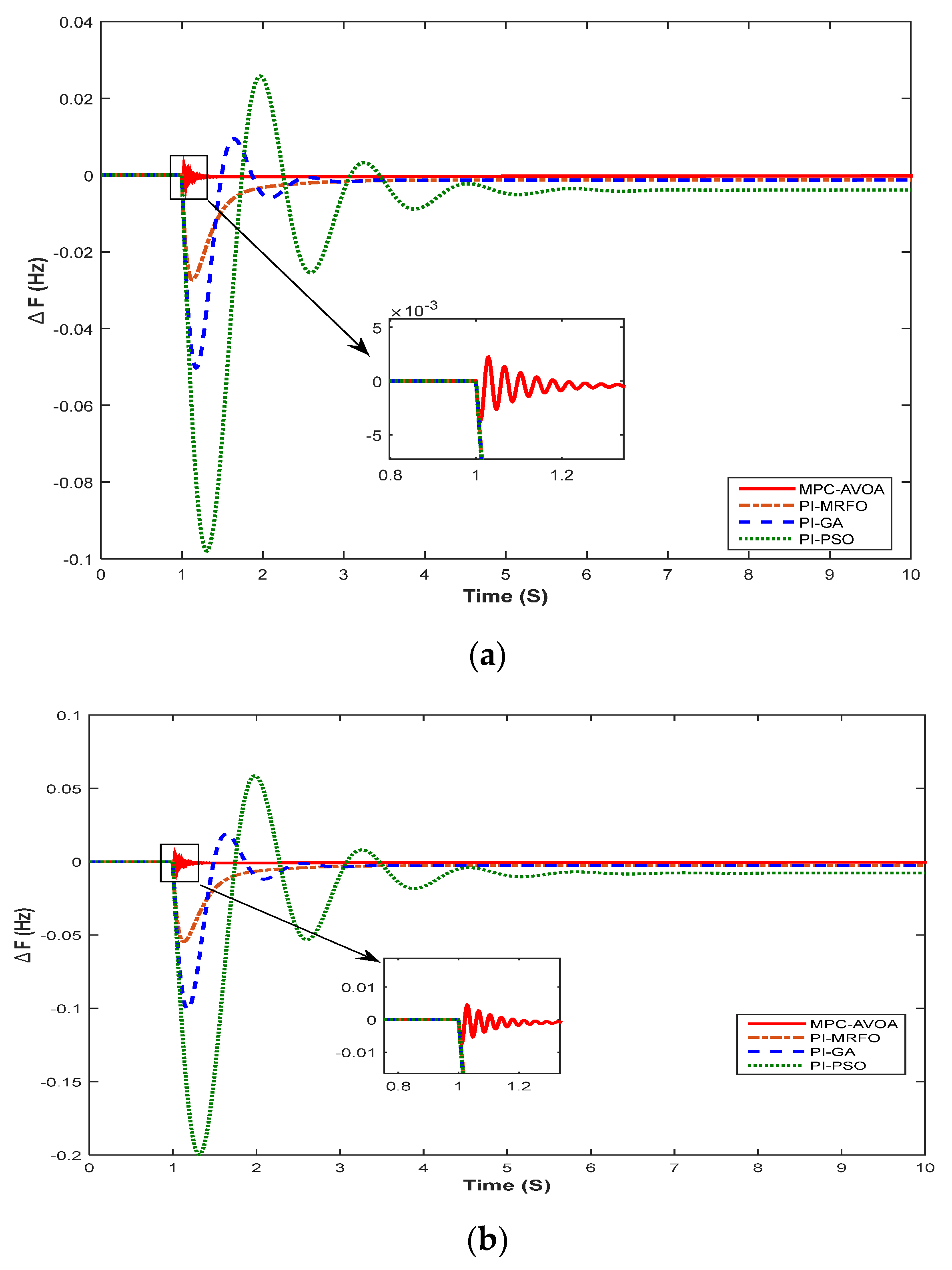
5.3. Scenario 2: Evaluation of Microgrid Performance under Reduced Microgrid Inertia

Step load disturbances of 5% and 10% are applied to the studied system at a time (t = 1 s) under a 50% decrease in the microgrid equivalent inertia. In this scenario, the reduced microgrid inertia is considered uncertain to the system for examining the islanded microgrid performance during demand changes and system uncertainties. The system frequency responses under 5% and 10% load disturbances during low system inertia are indicated in Figure 11a,b. These figures show that frequency changes of the islanded microgrid are more significant in oscillations and more remarkable in transient frequency deviation in the case of low inertia. The transient specifications for this scenario are introduced in Table 4. According to the transient parameters indicated in

Table 5. Transient specifications for Scenario 2.

Algorithm	SLP	HPSC (Hz)	LPSC (Hz)	TOS(s)	SSE (Hz)
MPC-AVOA	5%	0.0022	0.0037	0	0
PI-MRFO		0	0.0273	1.28	0.0012
PI-GA		0.0094	0.0502	138	0.0015
PI-PSO		0.026	0.098	2.75	0.0039
MPC-AVOA	10%	0.0045	0.0075	0	0
PI-MRFO		0	0.0545	1.48	0.0026
PI-GA		0.019	0.1005	1.65	0.0028
PI-PSO		0.059	0.2	3.12	0.0079

and considering the disturbance alleviation purpose, error minimization, and reference tracking property, it can be noticed that a more favorable result is attained by the AVOA-based MPC controller in the virtual inertial control loop. The simulation outcomes show that the optimal MPC performs better in tracking the frequency zero references during different step load disturbances in case of reduced microgrid inertia compared to the conventional PI controller with various optimization algorithms.

5.4. Scenario 3: Evaluation of Microgrid Performance with RES

Fluctuations in RES intermittent power and continuous changes in the load power are considered two essential characteristics of the isolated network. Thus, in this section, the microgrid frequency evaluation is examined under solar and wind farm penetration in addition to the implementation of random load fluctuations. For achieving practical and real analysis, actual wind power data were collected and extracted from a wind power plant located in Al-Zaafrana, Egypt in 2014 [55]. The changes in real wind power are introduced in Figure 12a, in which the rated output power of the wind farm is specified as 0.4 p.u. MW, and the rated wind speed of the wind turbines is 15 m/s. The wind power fluctuates with a peak value of 0.3 p.u. MW below its rated power. In addition, experimental solar power data are collected for a full sunny day from a field test located in Riyadh, Saudi Arabia [55]. The solar data are extracted and imported into the Simulink model. The obtained solar power pattern is depicted in Figure 12b, in which the active solar power fluctuates smoothly until it reaches its peak power of 0.23 p.u. MW below the rated power, which is specified as 0.32 p.u. MW. Furthermore, Figure 12c demonstrates random load power changes during one whole day [56]. To achieve multiple strategies of the studied microgrid, a variety of working situations are depicted in

Table 6. Multiple operating conditions of the studied microgrid.

Disruption	Starting Time (Minutes)	Stopping Time (Minutes)	Size (MW)
Wind farm	400	-	10 MW
Solar farm	initial	-	8 MW
Domestic load	initial	900	15 MW

to examine the effectiveness of the AVOA-based MPC with the virtual inertial controller in case of high-RES penetration, demand power fluctuations, and overall system inertia changes.

The microgrid performance is examined under typical system inertia in this scenario. The studied microgrid frequency changes are depicted in Figure 13 under RES and load disturbances. The fluctuations in solar, wind, and load power increase the frequency disturbances compared to other scenarios. A complete comparison is made between AVOA-based MPC and conventional PI controllers by making a zoomed view during the connection of the wind farm at t = 400 min and disconnection of electric loads at t = 900 min.

Table 7. Evaluation parameters of system frequency for Scenario 3.

Controller	Maximum Overshoot (HZ)	Minima Overshoot (HZ)
AVOA-MPC	0.01	0.008
MRFO-PI	0.061	0.057
GA-PI	0.1	0.092
PSO-PI	0.19	0.16

depicts the different evaluation indices of the studied system in the case of different controllers. The PSO-based PI controller can regulate the deviation in the frequency within $\pm$0.2 Hz, while the system frequency is kept in the range of $\pm$0.1 Hz using a GA-based PI controller. In addition, the PI controller with the MRFO algorithm is able to keep the microgrid frequency deviation within ±0.05 Hz. On the other hand, the best result is obtained using the AVOA-based MPC, for which the proposed controller succeeded in regulating the microgrid frequency within $\pm$0.01 Hz under different operating conditions of the studied microgrid.

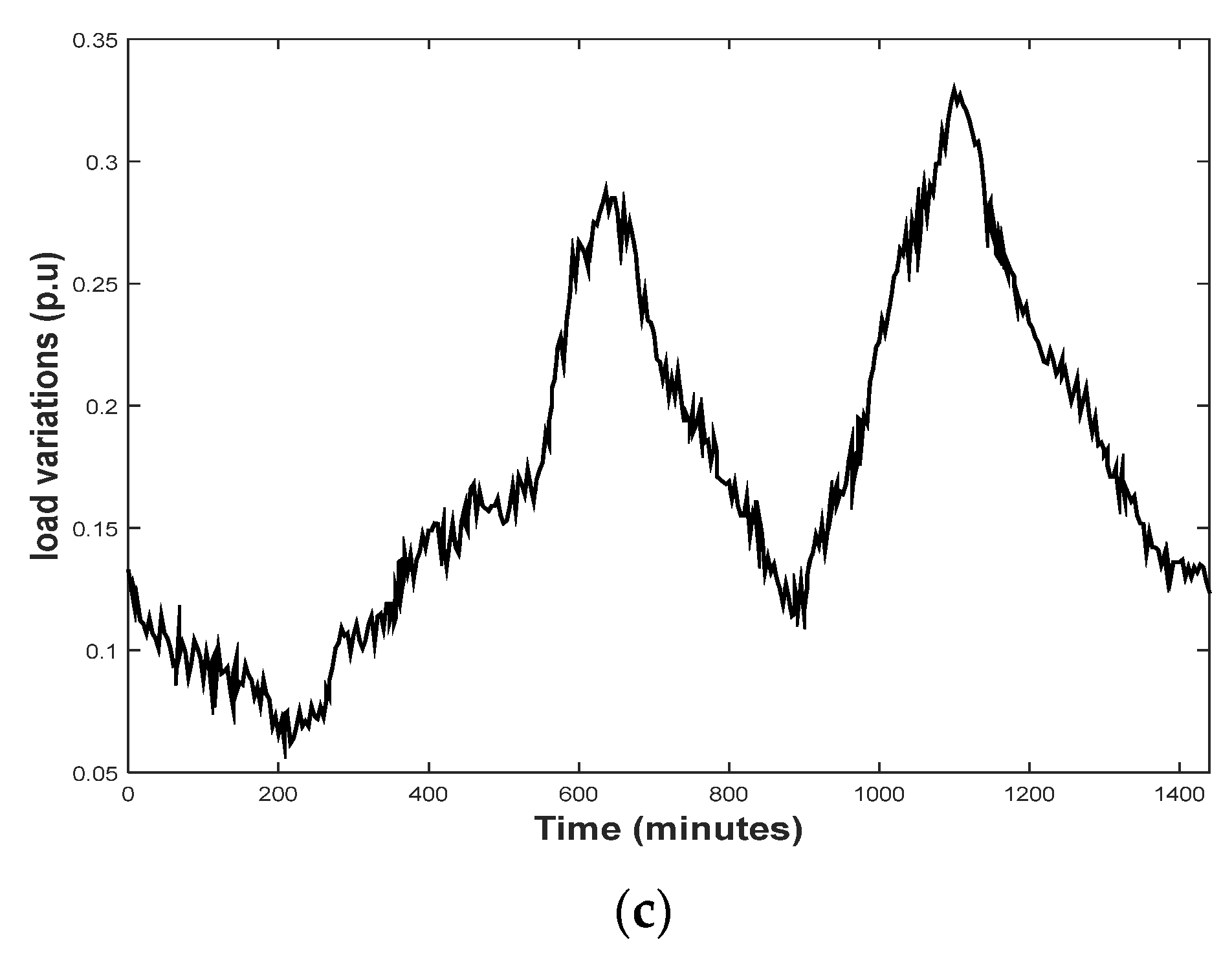
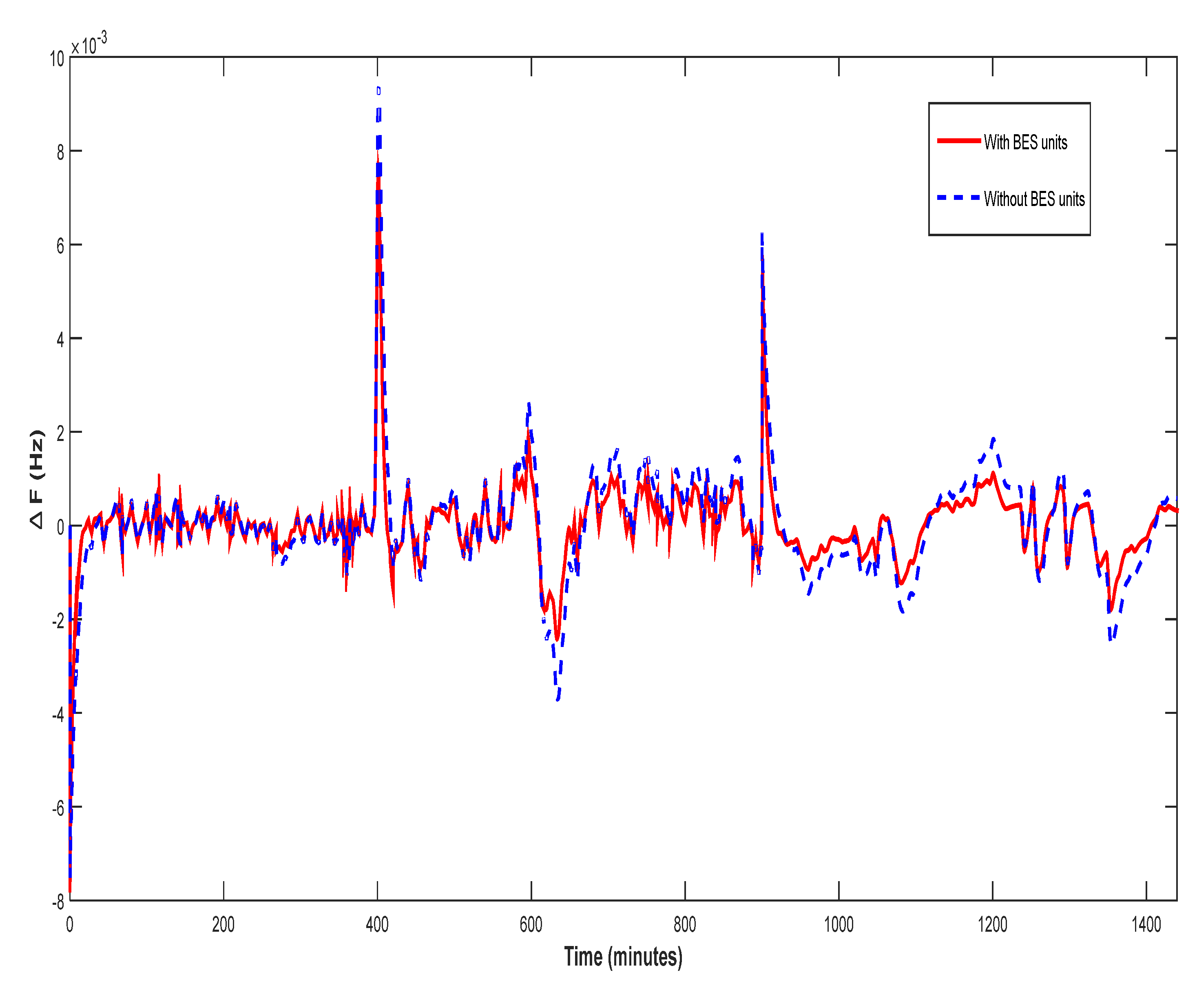
5.5. Scenario 4: Evaluation of Microgrid Performance with RES and BES Units

In this scenario, the microgrid performance is examined considering the penetration of RES in addition to the effect of energy storage units. In this study, battery energy storage (BES) units of 8 MW rated power are utilized and connected to the microgrid as introduced in Figure 2. The conventional PI controller is used to produce the dispatched frequency control signal to provide the damping signal from the BES. The power patterns of solar, wind, and load in Figure 12 are also implemented in this scenario. The microgrid performance is also investigated under the multiple operations shown in Table 6. The primary objective of this scenario is to demonstrate the energy storage units’ significant impact in dampening the studied microgrid’s frequency oscillations. Figure 14 depicts the studied system frequency fluctuations with and without the impact of the BES units. It can be noticed that the microgrid frequency fluctuations are significantly damped. During the connection of the wind farm at t = 400 min, frequency overshoot reaches 0.01 Hz without the effect of BES. While considering the effect of BES, the frequency overshoot is limited to 0.007 Hz. Moreover, during the disconnection of the electric loads at t = 900 min, the frequency deviation reaches 0.007 Hz without the BES’s impact. On the other hand, the frequency overshoot is limited to 0.005 Hz considering the effect of BES. The BES units improve the isolated microgrid frequency resilience, and this is because of the significant active power which is injected by the storage units.

6. Conclusions

As the RES penetration level increases, the lack of network inertia negatively affects islanded microgrids, leading to frequency instability and cascading outages in the worst-case scenario. This is a pressing issue regarding the increasing amount of RES being installed in electric grids now and in the future. In this study, model predictive control (MPC) is employed in the virtual inertial control loop to support frequency stability in an isolated microgrid with high penetration of RES. The optimal design of MPC is attained using the African Vultures Optimization Algorithm (AVOA). The AVOA-based MPC is designed to reduce the impact of RES power variation, load fluctuations, and system perturbations (i.e., overall microgrid inertia). Furthermore, the system contains battery energy storage (BES) units to enhance the transient stability of the islanded microgrid. The simulation outcomes prove the efficacy of the proposed optimal MPC controller in regulating the system frequency and attenuating the frequency oscillations compared to a conventional PI controller that is optimally designed using different optimization algorithms. Moreover, the time domain simulation outcomes show the significant role of BES in improving the transient frequency stability and alleviating the frequency disturbances in isolated microgrids.

References

1. Cheema, K.M. A comprehensive review of virtual synchronous generator. Int. J. Electr. Power Energy Syst. 2020, 120, 106006. [Google Scholar] [CrossRef]
2. Chandak, S.; Rout, P.K. The implementation framework of a microgrid: A review. Int. J. Energy Res. 2020, 45, 3523–3547. [Google Scholar] [CrossRef]
3. Palaniappan, R.; Molodchyk, O.; Shariati-Sarcheshmeh, M.; Asmah, M.W.; Liu, J.; Schlichtherle, T.; Richter, F.; Kwofie, E.A.; Festner, D.R.; Blanco, G.; et al. Experimental verification of smart grid control functions on international grids using a real-time simulator. IET Gener. Transm. Distrib. 2022, 16, 2747–2760. [Google Scholar] [CrossRef]
4. Rehman, H.U.; Yan, X.; Abdelbaky, M.A.; Jan, M.U.; Iqbal, S. An advanced virtual synchronous generator control technique for frequency regulation of grid-connected PV system. Int. J. Electr. Power Energy Syst. 2021, 125, 106440. [Google Scholar] [CrossRef]
5. Zakir, M.; Arshad, A.; Sher, H.A.; Al-Durra, A. Design and implementation of a fault detection method for a PV-fed DC-microgrid with power control mechanism. IET Electr. Power Appl. 2022, 16, 1057–1071. [Google Scholar] [CrossRef]
6. Karimi, A.; Khayat, Y.; Naderi, M.; Dragicevic, T.; Mirzaei, R.; Blaabjerg, F.; Bevrani, H. Inertia Response Improvement in AC Microgrids: A Fuzzy-Based Virtual Synchronous Generator Control. IEEE Trans. Power Electron. 2019, 35, 4321–4331. [Google Scholar] [CrossRef]
7. Gherairi, S. Design and implementation of an intelligent energy management system for smart home utilizing a multi-agent system. Ain Shams Eng. J. 2022, 14, 101897. [Google Scholar] [CrossRef]
8. Kim, H.-J.; Kim, M.-K. Multi-Objective Based Optimal Energy Management of Grid-Connected Microgrid Considering Advanced Demand Response. Energies 2019, 12, 4142. [Google Scholar] [CrossRef] [Green Version]
9. Zakir, M.; Sher, H.A.; Arshad, A.; Lehtonen, M. A fault detection, localization, and categorization method for PV fed DC-microgrid with power-sharing management among the nano-grids. Int. J. Electr. Power Energy Syst. 2022, 137, 107858. [Google Scholar] [CrossRef]
10. Li, L.; Chen, W.; Han, Y.; Li, Q.; Pu, Y. A Stability Enhancement Method Based on Adaptive Virtual Resistor for Electric-hydrogen Hybrid DC Microgrid Grid-connected Inverter Under Weak Grid. Electr. Power Syst. Res. 2021, 191, 106882. [Google Scholar] [CrossRef]
11. Mokhtar, M.; Marei, M.I.; Attia, M.A. Hybrid SCA and adaptive controller to enhance the performance of grid-connected PV system. Ain Shams Eng. J. 2021, 12, 3775–3781. [Google Scholar] [CrossRef]
12. Willenberg, D.; Winkens, A.; Linnartz, P. Impact of wind turbine generator technologies and frequency controls on the stable operation of medium voltage islanded microgrids. Electr. Power Syst. Res. 2020, 189, 106760. [Google Scholar] [CrossRef]
13. Kerdphol, T.; Watanabe, M.; Mitani, Y.; Turschner, D.; Beck, H.P. Stability Assessment of Multiple Virtual Synchronous Machines for Microgrid Frequency Stabilization. In Proceedings of the 2020 IEEE Power & Energy Society General Meeting (PESGM), Montreal, QC, Canada, 2–6 August 2020; IEEE: Piscataway, NJ, USA, 2020. [Google Scholar]
14. Hou, X.; Sun, Y.; Zhang, X.; Lu, J.; Wang, P.; Guerrero, J.M. Improvement of Frequency Regulation in VSG-Based AC Microgrid Via Adaptive Virtual Inertia. IEEE Trans. Power Electron. 2019, 35, 1589–1602. [Google Scholar] [CrossRef]
15. Mallemaci, V.; Mandrile, F.; Rubino, S.; Mazza, A.; Carpaneto, E.; Bojoi, R. A comprehensive comparison of Virtual Synchronous Generators with focus on virtual inertia and frequency regulation. Electr. Power Syst. Res. 2021, 201, 107516. [Google Scholar] [CrossRef]
16. Xiong, X.; Wu, C.; Blaabjerg, F. An improved synchronization stability method of virtual synchronous generators based on frequency feedforward on reactive power control loop. IEEE Trans. Power Electron. 2021, 36, 9136–9148. [Google Scholar] [CrossRef]
17. Liu, R.; Wang, S.; Liu, G.; Wen, S.; Zhang, J.; Ma, Y. An Improved Virtual Inertia Control Strategy for Low Voltage AC Microgrids with Hybrid Energy Storage Systems. Energies 2022, 15, 442. [Google Scholar] [CrossRef]
18. Fathi, A.; Shafiee, Q.; Bevrani, H. Robust Frequency Control of Microgrids Using an Extended Virtual Synchronous Generator. IEEE Trans. Power Syst. 2018, 33, 6289–6297. [Google Scholar] [CrossRef]
19. Saxena, P.; Singh, N.; Pandey, A.K. Enhancing the dynamic performance of microgrid using derivative controlled solar and energy storage based virtual inertia system. J. Energy Storage 2020, 31, 101613. [Google Scholar] [CrossRef]
20. Kerdphol, T.; Rahman, F.S.; Watanabe, M.; Mitani, Y.; Turschner, D.; Beck, H.-P. Enhanced Virtual Inertia Control Based on Derivative Technique to Emulate Simultaneous Inertia and Damping Properties for Microgrid Frequency Regulation. IEEE Access 2019, 7, 14422–14433. [Google Scholar] [CrossRef]
21. Kerdphol, T.; Watanabe, M.; Hongesombut, K.; Mitani, Y. Self-Adaptive Virtual Inertia Control-Based Fuzzy Logic to Improve Frequency Stability of Microgrid with High Renewable Penetration. IEEE Access 2019, 7, 76071–76083. [Google Scholar] [CrossRef]
22. Ali, H.; Magdy, G.; Li, B.; Shabib, G.; Elbaset, A.A.; Xu, D.; Mitani, Y. A New Frequency Control Strategy in an Islanded Microgrid Using Virtual Inertia Control-Based Coefficient Diagram Method. IEEE Access 2019, 7, 16979–16990. [Google Scholar] [CrossRef]
23. Kerdphol, T.; Rahman, F.S.; Mitani, Y.; Watanabe, M.; Küfeoğlu, S.K. Robust Virtual Inertia Control of an Islanded Microgrid Considering High Penetration of Renewable Energy. IEEE Access 2017, 6, 625–636. [Google Scholar] [CrossRef]
24. Ali, H.; Magdy, G.; Xu, D. A new optimal robust controller for frequency stability of interconnected hybrid microgrids considering non-inertia sources and uncertainties. Int. J. Electr. Power Energy Syst. 2021, 128, 106651. [Google Scholar] [CrossRef]
25. Kerdphol, T.; Watanabe, M.; Mitani, Y.; Phunpeng, V. Applying Virtual Inertia Control Topology to SMES System for Frequency Stability Improvement of Low-Inertia Microgrids Driven by High Renewables. Energies 2019, 12, 3902. [Google Scholar] [CrossRef] [Green Version]
26. Magdy, G.; Bakeer, A.; Nour, M.; Petlenkov, E. A New Virtual Synchronous Generator Design Based on the SMES System for Frequency Stability of Low-Inertia Power Grids. Energies 2020, 13, 5641. [Google Scholar] [CrossRef]
27. Saleh, A.; Omran, W.A.; Hasanien, H.M.; Tostado-Véliz, M.; Alkuhayli, A.; Jurado, F. Manta Ray Foraging Optimization for the Virtual Inertia Control of Islanded Microgrids Including Renewable Energy Sources. Sustainability 2022, 14, 4189. [Google Scholar] [CrossRef]
28. Magdy, G.; Shabib, G.; Elbaset, A.A.; Mitani, Y. A Novel Coordination Scheme of Virtual Inertia Control and Digital Protection for Microgrid Dynamic Security Considering High Renewable Energy Penetration. IET Renew. Power Gener. 2019, 13, 462–474. [Google Scholar] [CrossRef]
29. Skiparev, V.; Machlev, R.; Chowdhury, N.; Levron, Y.; Petlenkov, E.; Belikov, J. Virtual Inertia Control Methods in Islanded Microgrids. Energies 2021, 14, 1562. [Google Scholar] [CrossRef]
30. Bordons, C.; Garcia-Torres, F.; Ridao, M.A. Model Predictive Control of Microgrids; Springer: Cham, Switzerland, 2020; Volume 358. [Google Scholar]
31. Sun, Q.; Zhang, K.; Shi, Y. Resilient Model Predictive Control of Cyber–Physical Systems Under DoS Attacks. IEEE Trans. Ind. Informatics 2019, 16, 4920–4927. [Google Scholar] [CrossRef]
32. Di Cairano, S.; Kolmanovsky, I.V. Real-time optimization and model predictive control for aerospace and automotive applications. In Proceedings of the 2018 Annual American Control Conference (ACC), Milwaukee, WI, USA, 27–29 June 2018; IEEE: Piscataway, NJ, USA, 2018. [Google Scholar]
33. Hu, J.; Shan, Y.; Guerrero, J.M.; Ioinovici, A.; Chan, K.W.; Rodriguez, J. Model predictive control of microgrids—An overview. Renew. Sustain. Energy Rev. 2021, 136, 110422. [Google Scholar] [CrossRef]
34. Nelson, J.R.; Johnson, N.G. Model predictive control of microgrids for real-time ancillary service market participation. Appl. Energy 2020, 269, 114963. [Google Scholar] [CrossRef]
35. Jan, M.U.; Xin, A.; Rehman, H.U.; Abdelbaky, M.A.; Iqbal, S.; Aurangzeb, M. Frequency regulation of an isolated microgrid with electric vehicles and energy storage system integration using adaptive and model predictive controllers. IEEE Access 2021, 9, 14958–14970. [Google Scholar] [CrossRef]
36. Gbadega, P.A.; Saha, A.K. Load Frequency Control of a Two-Area Power System with a Stand-Alone Microgrid Based on Adaptive Model Predictive Control. IEEE J. Emerg. Sel. Top. Power Electron. 2020, 9, 7253–7263. [Google Scholar] [CrossRef]
37. Kerdphol, T.; Rahman, F.S.; Mitani, Y.; Hongesombut, K.; Küfeoğlu, S. Virtual Inertia Control-Based Model Predictive Control for Microgrid Frequency Stabilization Considering High Renewable Energy Integration. Sustainability 2017, 9, 773. [Google Scholar] [CrossRef] [Green Version]
38. Abdollahzadeh, B.; Gharehchopogh, F.S.; Mirjalili, S. African vultures optimization algorithm: A new nature-inspired metaheuristic algorithm for global optimization problems. Comput. Ind. Eng. 2021, 158, 107408. [Google Scholar] [CrossRef]
39. Wang, Y.; Li, S.; Sun, H.; Huang, C.; Youssefi, N. The utilization of adaptive African vulture optimizer for optimal parameter identification of SOFC. Energy Rep. 2022, 8, 551–560. [Google Scholar] [CrossRef]
40. Wang, Y.; Wang, J.; Yang, L.; Ma, B.; Sun, G.; Youssefi, N. Optimal designing of a hybrid renewable energy system connected to an unreliable grid based on enhanced African vulture optimizer. ISA Trans. 2022, 129, 424–435. [Google Scholar] [CrossRef]
41. Kerdphol, T.; Rahman, F.S.; Mitani, Y. Virtual Inertia Control Application to Enhance Frequency Stability of Interconnected Power Systems with High Renewable Energy Penetration. Energies 2018, 11, 981. [Google Scholar] [CrossRef] [Green Version]
42. Lu, K.; Zhou, W.; Zeng, G.; Zheng, Y. Constrained population extremal optimization-based robust load frequency control of multi-area interconnected power system. Int. J. Electr. Power Energy Syst. 2019, 105, 249–271. [Google Scholar] [CrossRef]
43. Alayi, R.; Zishan, F.; Seyednouri, S.R.; Kumar, R.; Ahmadi, M.H.; Sharifpur, M. Optimal Load Frequency Control of Island Microgrids via a PID Controller in the Presence of Wind Turbine and PV. Sustainability 2021, 13, 10728. [Google Scholar] [CrossRef]
44. Sobhy, M.A.; Abdelaziz, A.Y.; Hasanien, H.M.; Ezzat, M. Marine predators algorithm for load frequency control of modern interconnected power systems including renewable energy sources and energy storage units. Ain Shams Eng. J. 2021, 12, 3843–3857. [Google Scholar] [CrossRef]
45. Kerdphol, T.; Fuji, K.; Mitani, Y.; Watanabe, M.; Qudaih, Y. Optimization of a battery energy storage system using particle swarm optimization for stand-alone microgrids. Int. J. Electr. Power Energy Syst. 2016, 81, 32–39. [Google Scholar] [CrossRef]
46. Aditya, S.; Das, D. Battery energy storage for load frequency control of an interconnected power system. Electr. Power Syst. Res. 2001, 58, 179–185. [Google Scholar] [CrossRef]
47. Lu, C.F.; Liu, C.C.; Wu, C.J. Effect of battery energy storage system on load frequency control considering governor deadband and generation rate constraint. IEEE Trans. Energy Convers. 1995, 10, 555–561. [Google Scholar]
48. Cai, S.; Matsuhashi, R. Model Predictive Control for EV Aggregators Participating in System Frequency Regulation Market. IEEE Access 2021, 9, 80763–80771. [Google Scholar] [CrossRef]
49. Huang, H.; Xu, H.; Chen, F.; Zhang, C.; Mohammadzadeh, A. An Applied Type-3 Fuzzy Logic System: Practical Matlab Simulink and M-Files for Robotic, Control, and Modeling Applications. Symmetry 2023, 15, 475. [Google Scholar] [CrossRef]
50. Hassanpour, H.; Corbett, B.; Mhaskar, P. Artificial Neural Network-Based Model Predictive Control Using Correlated Data. Ind. Eng. Chem. Res. 2022, 61, 3075–3090. [Google Scholar] [CrossRef]
51. Bordons, C.; Garcia-Torres, F.; Ridao, M.A. Model Predictive Control Fundamentals. In Model Predictive Control of Microgrids; Springer: Cham, Switzerland, 2020; pp. 25–44. [Google Scholar]
52. Hussain, A.; Sher, H.A.; Murtaza, A.F.; Al-Haddad, K. Improved voltage controlled three phase voltage source inverter using model predictive control for standalone system. In Proceedings of the IECON 2018-44th Annual Conference of the IEEE Industrial Electronics Society, Washington, DC, USA, 21–23 October 2018; IEEE: Piscataway, NJ, USA, 2018. [Google Scholar]
53. Salah, B.; Hasanien, H.M.; Ghali, F.M.; Alsayed, Y.M.; Abdel Aleem, S.H.; El-Shahat, A. African Vulture Optimization-Based Optimal Control Strategy for Voltage Control of Islanded DC Microgrids. Sustainability 2022, 14, 11800. [Google Scholar] [CrossRef]
54. Pratap, A.; Tiwari, P.; Maurya, R.; Singh, B. Minimisation of electric vehicle charging stations impact on radial distribution networks by optimal allocation of DSTATCOM and DG using African vulture optimisation algorithm. Int. J. Ambient. Energy 2022, 43, 8653–8672. [Google Scholar] [CrossRef]
55. Hasanien, H.M. Whale optimisation algorithm for automatic generation control of interconnected modern power systems including renewable energy sources. IET Gener. Transm. Distrib. 2018, 12, 607–614. [Google Scholar] [CrossRef]
56. Lara-Santillán, P.M.; Mendoza-Villena, M.; Fernández-Jiménez, L.A.; Mañana-Canteli, M. A Comparative Study of Electric Load Curve Changes in an Urban Low-Voltage Substation in Spain during the Economic Crisis (2008–2013). Sci. World J. 2014, 2014, 948361. [Google Scholar] [CrossRef] [PubMed] [Green Version]
Figure 1. The studied microgrid conceptual structure with RES integration and BES system.
Sustainability 15 05009 g001
Figure 2. The studied microgrid dynamic model with virtual inertia control.
Sustainability 15 05009 g002
Figure 3. The virtual inertia control dynamic model with MPC.
Sustainability 15 05009 g003
Figure 4. Schematic depiction of the BES system.
Sustainability 15 05009 g004
Figure 5. Equivalent circuit representation of BES units.
Sustainability 15 05009 g005
Figure 6. BES incremental model design.
Sustainability 15 05009 g006
Figure 7. MPC general concept and strategy.
Sustainability 15 05009 g007
Figure 8. The conceptual structure of MPC.
Sustainability 15 05009 g008
Figure 9. AVOA flowchart.
Sustainability 15 05009 g009
Figure 10. System frequency response for scenario 1 (a) ∆f for 5% SLP, (b) ∆f for 10% SLP.
Sustainability 15 05009 g010
Figure 11. System frequency response for Scenario 2 (a) ∆f for 5% SLP, (b) ∆f for 10% SLP.
Sustainability 15 05009 g011
Figure 12. Wind, solar, and load power patterns: (a) wind power fluctuations, (b) solar power fluctuations, (c) load variation.
Sustainability 15 05009 g012aSustainability 15 05009 g012b
Figure 13. System frequency response for Scenario 3.
Sustainability 15 05009 g013
Figure 14. System frequency response for Scenario 4.
Sustainability 15 05009 g014