Abstract
As container ports become increasingly important to the global supply chain, a growing number of ports are improving their competencies by consolidating multiple terminal resources internally. In addition, in the context of energy conservation and emission reduction, ports measure competitiveness not only in terms of terminal size, throughput and service level, but also in terms of low energy consumption and low pollution. Therefore, a nonlinear mixed-integer programming model considering the cost of carbon is developed for the multi-terminal berth and quay crane joint robust scheduling problem under uncertain environments to minimize the sum of expectation and variance of total cost under all randomly generated samples. The model considers the water depth and interference of quay cranes, etc. The expected vessel arrival time and the average operational efficiency plus relaxation are used as their actual values when scheduling. Finally, an improved adaptive genetic algorithm is developed by combining the simulated annealing mechanism, and numerical experiments are designed. The results show that the joint berth and quay crane scheduling with uncertainties and a multi-terminal coordination mechanism can effectively reduce the operating cost, including carbon costs and the vessel departure delay rate, and can improve resource utilization. Meanwhile, the scheduling with the multi-terminal coordination mechanism can obtain more significant improvement effects than the scheduling with uncertainties.
1. Introduction
In recent years, container freight transport has developed rapidly due to its high efficiency; container ports have gradually become a vital node of the global supply chain, and their operational efficiency affects the efficiency of the entire supply chain. Due to geographical or other constraints, many ports exist with multiple terminals, such as the Port of Valencia, Keppel Terminal, Tanjong Pagar, and Blarney Terminal [1]. Terminals in these ports are usually operated by different entities and their resources cannot be shared with each other, so the efficiency cannot be maximized. With the increasing competition among ports, they must improve their competitiveness through the integration of resources. Furthermore, one of the major characteristics of maritime logistics is uncertainty. This will make the scheduling plan infeasible because of the constantly changing status of ships and terminals, such as arrival time, equipment breakdown, etc. The uncertainties mainly include arrival times, the operation time in the berth and the crane scheduling problem. In addition, changes in the operation time are usually caused by the quay crane operational efficiency or the breakdown of the quay crane, etc. In this paper, the influence yielded by the change in the quay crane operation efficiency is the focus. Furthermore, carbon emissions play a critical role in evaluating the operational efficiency of ports. Therefore, optimizing mechanical processes and resource allocation within ports is essential to reduce carbon emissions, promote energy conservation and emission reduction, foster the development of green port shipping, and enhance the competitiveness of port groups. This paper investigates the impact of berth and quay scheduling on carbon emissions.
At present, the field of container terminal frontier operation scheduling optimization already has many excellent review studies [2,3], and they have provided a relatively comprehensive description of relevant research in the field.
2. Literature Review
Many studies have focused on the independent scheduling of berths and quay cranes. De et al. [4] incorporated fuel consumption cost into the dynamic berth allocation problem and designed a chemical reaction optimization approach to solve it. Al-Refaie and Abedalqader [5] studied the berth allocation problem and proposed two optimization models under regular vessel arrivals and under emergency conditions, separately. Wawrzyniak et al. [6] investigated the algorithm selection problem for solving the berth allocation problem. Abou Kasm and Diabat [7] studied the scheduling problem in the application of a new quay crane. Lv et al. [8] established a mixed-integer linear programming model for the berth allocation recovery problem and solved it using the squeaky wheel optimization heuristic. Jia et al. [9] studied how to allocate berths to deep-sea vessels and schedule arrivals of feeders for congestion mitigation at a container port with a stochastic optimization model, and solved the problem by a three-phase simulation optimization method. Xiang et al. [10] developed a data-driven model to optimize berth allocation at container terminals considering uncertain operation time, using clustering and algorithm generation techniques, and demonstrated its effectiveness through computational experiments. Rodrigues et al. [11] provided a comprehensive survey of literature on berth allocation and quay crane assignment problems under uncertainty, classifying approaches into proactive, reactive, and identifying research trends, limitations, and future directions.
As a complex system, the internal parts of container ports interact with each other. Many studies are focused on the integrated scheduling problems of them. Some focused on the integrated quay crane and yard truck scheduling problem, such as Cao et al. [12]; others considered the simultaneous storage space and berth allocation problem, such as Safaei et al. [13] taking the form of a hybrid flow shop. Jonker et al. [14] developed a comprehensive model for the scheduling of quay cranes, AGVs, and yard cranes, and they also solved it by a tailored simulated annealing algorithm. Agra et al. [15] considered an integrated berth allocation and quay crane assignment and scheduling problem motivated by a real case where a heterogeneous set of cranes is considered. Li et al. [16] investigated an integrated berth allocation and quay crane assignment with uncertain quay crane maintenance activities and established a stochastic integer linear programming model to minimize the excepted total turnaround time of vessels. Chargui et al. [17] proposed a new extension of the berth and quay crane allocation and scheduling problems considering worker performance variability and yard truck deployment constraints. Ji et al. [18] solved the Berth Allocation and Quay Crane Assignment Problem (BACAP) with stochastic vessel arrival times using a scenario generation method and an MILP model to minimize the expected total vessel stay time. Tang et al. [19] proposed a mixed-integer linear programming model and a large neighborhood search algorithm to solve the continuous berth allocation and quay crane assignment problem, aiming to minimize the total stay time and delay penalty of ships. Most research has focused on the integrated berth and quay crane scheduling problem.
In realistic situations, the final scheduling solution may be infeasible if uncertainties are ignored during scheduling. Therefore, many scholars have conducted studies on resource scheduling in container terminals under uncertainties. These studies usually consider the uncertain arrival time and operation time, while they are different in strategies for coping with these uncertainties. Zhen and Chang [20] improved the robustness of the model by inserting buffer times between vessels and proposed a heuristic algorithm based on the squeaky wheel optimization method. Xiang et al. [21] examined the simultaneous allocation of berths and quay cranes under discrete berth situations with uncertainty at container terminals. Iris and Lam [22] applied recoverable robustness and designed an adaptive large neighborhood algorithm for solving the problem. Rodrigues and Agra [23] modeled the integrated berth allocation and scheduling problem under uncertain arrival time as a two-stage robust mixed-integer program and proposed a new scenario reduction procedure with a warm start technique to break down the problem.
In the context of a low-carbon economy, many experts have discussed the calculation of carbon cost in depth, mainly focusing on land transportation, maritime transportation and carbon costs of production enterprises, but relatively little research has been carried out on the carbon emission cost of ports. Prayogo et al. [24] discussed the model development of carbon emission cost in container terminal operations planning using a system dynamics approach. Sun et al. [25] considered a combination of the cost of all tasks, the total operating cost of quay cranes and the carbon taxation cost, and proposed a recoverable robustness berth and quay crane assignment-planning model. Lin et al. [26] investigates an integrated optimization problem of berths, quay cranes, and yard spaces allocation for tidal ports with channel capacity constraints under a carbon tax policy. Karam et al. [27] proposed a planning model that integrates berth allocation, quay crane assignment, and internal truck assignment problems with energy-saving goals and realistic factors.
To the best of the authors’ knowledge, few studies have focused on frontier operation scheduling problems for the multi-terminal container port. Imai et al. [28] took Colombo port as an example and studied the berth allocation problem when berths in other terminals could be shared. Krimi et al. [29] presented an efficient rolling horizon-based heuristic to solve the integrated berth allocation and crane assignment problem in bulk ports. Bouzekri et al. [30] focus on the integrated laycan and berth allocation and quay crane assignment problem for tidal ports with multiple quays and different water depths; they proposed two models for the integration of the time-invariant quay crane assignment and the specific quay crane assignment, separately. Martin-Iradi et al. [31] consider a variant of the berth allocation problem—that is, the multiport berth allocation problem—aimed at assigning berthing times and positions to vessels in container terminals. In fact, their research is very similar to ours. However, they ignored the uncertainty in the terminals and did not consider the carbon emissions of these terminals, which are important factors when assigning berthing positions to ships. In addition, they used CPLEX to solve small instances, but did not provide an algorithm for large instances.
From previous studies, it can be seen that, the research on berth allocation and quay crane assignment under a low-carbon background is relatively insufficient. There are few studies on multiple terminals considering carbon emission reduction. Furthermore, most studies only consider a defined environment, without considering the uncertain arrival times and quay crane operational efficiency. Therefore, besides considering water depth, interference between quay cranes and export container transportation, this paper investigates the multi-terminal continuous berth and quay cranes robust scheduling problem with uncertain arrival times and quay crane operational efficiency. It can provide a little theoretical basis for the intensive operation of ports where multiple container terminals exist.
3. Problem Description and Formulation
The usual operation processes of a container terminal are shown in Figure 1. From the ship’s point of view, if the ship needs to berth at the terminal, it should inform the terminal in advance of the length, expected arrival time, stowage plan, etc. Then, its berthing position, berthing time, specific operation quay cranes, and operational sequence of tasks will be determined by the terminal. After all tasks are completed, the ship leaves the port. Berth allocation, quay crane assignment, and quay crane scheduling involved in this process are considered seaside operations.
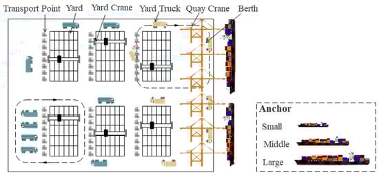
Figure 1.
Container terminal workflow.
From the container point of view, after being unloaded from the ship by the quay crane (or when the container owner needs to send it out), it will be transported to the assigned yard by truck and then placed at the assigned option through the yard crane. When the container owner needs it (or it needs to be loaded onto the ship), it will be taken out using the yard cranes and be transported to the owner by truck (or be sent to the quay crane and loaded onto the ship). The landside operations of this process encompass yard truck scheduling, storage space allocation, and yard crane scheduling.
In this paper, we assume a container port with terminals, each terminal with independent natural conditions and resources, such as the length of the quay , the water depth , the number of quay cranes , etc. During the planning period H, ships will arrive, each ship with a different draft , expected arrival time , expected departure time , etc. In addition, there are already vessels in the terminals at the beginning of the planning period. The actual arrival time and the actual efficiency of cranes are defined as random variables with normal distribution. In addition, samples are generated according to the distribution function. For each vessel, a penalty cost is incurred if its actual arrival time exceeds its scheduled berthing time or if its actual departure time exceeds its expected departure time . The penalty cost is a measure of the deviation from the planned schedule and is used to discourage such deviations and promote adherence to the scheduled time frames. When the vessel’s actual berthing terminal does not coincide with the pre-assigned terminal , the export containers need to be transferred to the actual berthing terminal. In practice, if the ship deviates from the preferred berth, the container will be transported from the container truck to the corresponding yard and container area of the preferred berth, then the carbon dioxide emissions will be generated. In the context of this problem, the berthing terminal , berthing position , berthing time , and the number of quay cranes assigned are determined to minimize the expected value and the standard deviation of the total cost for all ships across all samples.
3.1. Model Assumptions and Notation
- Berths are uninterrupted and vessels may dock at any point along the quay, provided that they meet the necessary requirements;
- Terminals have different water depths, and vessels can only berth at terminals that meet their draft;
- All quay cranes on the same terminal are located on the same track and cannot change or serve across terminals;
- The minimum and maximum number of quay cranes for each vessel are required, and the actual operational efficiency of the quay cranes will decrease when multiple quay cranes are working on the same vessel together.
The constant in the model are as Table 1, and the decision variables and Auxiliary decision variables are as Table 2.

Table 1.
Constant definition.
Table 1.
Constant definition.
| Type | Symbol | Definition |
|---|---|---|
| Constants | Set of terminals, | |
| Set of vessels to be scheduled, | ||
| Set of vessels berthed before planning period, | ||
| Set of quay cranes at the terminal , , | ||
| Set of samples; each represents the actual arrival time, the quay crane operational efficiency and the actual departure time, | ||
| Length of quay at the terminal , | ||
| Water depth at the terminal , | ||
| Expected operational efficiency of quay cranes at the terminal , | ||
| Interference factor between quay cranes | ||
| Length of the berthed vessel , including safety distance, | ||
| Berthing position of the berthed vessel , | ||
| If the berthing terminal of the berthed vessel is , ; otherwise, , , | ||
| Number of unfinished containers for the berthed vessel , | ||
| If the quay crane located at terminal serves the berthed vessel , ; otherwise, , , , | ||
| Length of the vessel , including safety distance, | ||
| If the pre-assigned terminal of the vessel is , ; otherwise, , , | ||
| Number of containers exported on the vessel , | ||
| Number of containers imported on the vessel , | ||
| Expected arrival time of the vessel , | ||
| Expected departure time of the vessel , | ||
| Minimum number of quay cranes assigned to the vessel , | ||
| Maximum number of quay cranes assigned to the vessel , | ||
| Draft of the vessel , | ||
| Desired berthing position of the vessel at its pre-assigned terminal, | ||
| Deviation cost per meter between vessel’s berthing position and its desired position | ||
| Operation costs per hour for a quay crane | ||
| Transshipment costs per container from terminal to terminal , | ||
| Penalty cost per hour when the actual departure time of vessel exceeds its expected departure time, | ||
| Waiting cost per hour when actual arrival time earlier than scheduling berthing time | ||
| Penalty cost per hour when actual arrival time later than scheduling berthing time | ||
| A sufficiently large positive number |
Table 2.
Variable definition.
Table 2.
Variable definition.
| Type | Symbol | Definition |
|---|---|---|
| Decision variables | If the berthing terminal of vessel is , ; otherwise, , , | |
| Berthing position of vessel , | ||
| Berthing time of vessel , | ||
| If the quay crane at terminal serves the vessel , ; otherwise, , , , | ||
| Auxiliary decision variables | Relaxation with arrival times of vessel , | |
| Relaxation with the operational efficiency of quay crane serving vessel , | ||
| Number of quay crane serving vessel , | ||
| Scheduling departure time of vessel | ||
| If the vessel berths after the departure time of vessel , ; otherwise, , , | ||
| If the vessel berths to the right of vessel , ; otherwise, , , | ||
| If the vessel berths after the departure time of berthed vessel , ; otherwise,, , | ||
| If the vessel berths to the right of berthed vessel , ; otherwise, , , | ||
| If the vessel berths to the left of berthed vessel , ; otherwise, , , |
Chat Source: journal of marine science and engineering [32].
3.2. Cost of Carbon Calculation
To calculate the carbon emission cost of the port, we primarily consider the additional carbon emissions resulting from the ship deviating from its pre-assigned berth. When a ship fails to dock at the pre-assigned berth, its containers must be transported to the pre-assigned terminal using container trucks, which incurs an associated carbon emission cost.
In (1), denotes the cost of carbon emissions per unit distance for container trucks, measured in US dollars per meter. represents the fuel consumption rate per unit distance of the collector truck (primarily diesel for container trucks) measured in tons per kilometer. represents the low heating value of diesel fuel, measured in megajoules per ton of fuel. represents the fuel emission factor measured in grams of carbon dioxide per megajoule of energy produced. represents the unit cost of carbon dioxide (CO2) emissions, measured in US dollars per ton.
3.3. Objective Function
With the objective function, referring to the literature [33], first, we generated a certain number of samples, each with the actual arrival time, quay crane operational efficiency, and actual departure time for all vessels. Then, we calculated the total cost for all vessels in the scheduling plan under each sample. Finally, we minimize the expectation plus the standard deviation of the total cost under all samples as the objective function, as shown in (2) and (3).
In (3), represents the operational cost. refers to the waiting cost incurred when the actual arrival time of a vessel is earlier than its scheduled berthing time. In case a vessel arrives before its scheduled berthing time, it is required to anchor and wait, which results in lower satisfaction for the vessel and potentially affects the port’s competitiveness. represents the penalty imposed when a ship’s actual arrival time exceeds its scheduled berthing time, resulting in delays that negatively impact the port’s efficiency and customer satisfaction. denotes the penalty cost incurred when the actual departure time of a vessel is later than its expected departure time. Ensuring smooth departure is crucial for both ships and terminals. Failure to depart on time may result in delay in reaching the next port for the ship, and disrupt the berthing and operations of subsequent ships for the terminal. represents the transshipment cost incurred due to the deviation between the actual terminal used and the pre-assigned terminal for each vessel. represents the carbon emissions cost associated with deviations between the desired berthing position and the actual berthing position of a vessel.
3.4. Constraints
The objective function plays a critical role in determining the most optimal scheduling scheme. However, it is essential to take into account numerous constraints to obtain a practical and feasible ship berthing plan and shore bridge allocation plan.
In our model, there exist constraints that require consideration in addition to the objective function. In the case of berthing terminals, it is necessary to ensure that each ship only berth at one terminal, as shown in (4). In addition, (5) ensures that the water depth of the terminal where each vessel berths meets its draft.
There are also constraints on berthing positions for all vessels. Firstly, as shown in (6), the position for a vessel to berth must be within the quay of the terminals. Secondly, it is also necessary to ensure that no two vessels occupy the same section of terminal at the same time, as shown in (7)–(9).
There are also several constraints on the berthing time. The vessel’s arrival time and quay crane operational efficiency are usually uncertain and obey a normal distribution, i.e., and , which changes the berthing time and makes the scheduling plan infeasible. Therefore, to minimize the impact of these uncertainties without rescheduling, we consider the sum of the expected value and relaxation as the arrival time during scheduling and employ the same approach for the quay crane operational efficiency. As shown in (10), all vessels must berth after their arrival. In (1), the relationship between the vessel’s departure time, berthing time, and quay crane operational efficiency is defined. In addition, as shown in (12) and (13), when any two ships do not berth at the same terminal at the same time, it is also necessary to ensure the relationship between their berthing time and departure time.
In addition to the above constraints, if any two vessels berth at the same terminal, they must have a left–right relationship in berthing position or a sequential relationship in berthing time. If not, there is a risk of simultaneous occupation of the same section of the quay, necessitating the use of Equations (14) and (15).
Several constraints on quay cranes must be satisfied, too. Firstly, Equation (16) specifies a minimum and maximum number of quay cranes that can be assigned to each vessel. At the same time, (17) ensures the quay cranes serving a vessel belong to the terminal where the vessel berths. In addition, as shown in (18) and (19), each quay crane serves at most one vessel at the same time; (20) indicates that the serial number of quay cranes serving one vessel must be consecutive. Finally, (21)–(23) ensure that the quay cranes cannot cross each other or cross terminals to serve any two vessels berthing together.
4. Solution Method
The multi-terminal continuous berth and quay crane scheduling problem with uncertainties is more complex than the berth allocation problem, which is already an NP-hard problem. It is hard to find the optimal solution in polynomial time for large-scale problems. Thus, this study proposes an adaptive improved genetic algorithm, which integrates a simulated annealing mechanism (SA-AGA) to solve the problem. Figure 2 shows the flow chart of our algorithm.
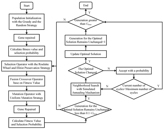
Figure 2.
The flow chart of the SA-AGA.
4.1. Encoding & Decoding Rules
How to encode the solution of a problem as a chromosome is a vital problem in applications of the genetic algorithm. In this paper, as shown in Figure 3, we adopt the real number encoding method and use a matrix of size 7N_V to represent a solution.
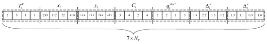
Figure 3.
An example of the chromosome represented as a solution.
The genetic block corresponds to the serial number of vessels. The first three segments of the genetic block correspond to the berth’s terminal , position , and time for each vessel. The fourth and fifth segments of the genetic block represent the number of assigned quay cranes and the serial number of the first assigned quay crane . The last two segments indicate the relaxation of the arrival time and the operational efficiency , separately.
Taking Figure 3 as an example, the first vessel berths at 233 m from the second terminal at 12.8 (=11.4 + 1.4) and is served by quay cranes from 2 to 4. The quay crane operational efficiency is the expected efficiency plus relaxation ( + 1.3). Similarly, the second vessel berths at 112 m from the third terminal at 15.5 (=13.3 + 2.2) and is served by quay cranes from 2 to 5. The quay crane operational efficiency is the expected efficiency plus the slack ( + 1.1), followed by the following.
4.2. Population Initialization
If the initial solution is of higher quality, the population may evolve to a better state after fewer iterations. Otherwise, it will take longer to approach the optimal solution, and the algorithm can be less efficient. At the same time, the diversity of the initial population makes it more possible to approach the optimal solution and easier to jump out of the local optimum. Therefore, this paper uses the greedy construction strategy to obtain the initial population combining the random generation strategy.
On the one hand, half of the initial population is generated using the greedy construction strategy. First, the pre-assigned terminal is designated as the berthing terminal, and the desired berthing position is assigned as the berthing position for each vessel. Then, the expected arrival time plus the initial relaxation of arrival time is considered as the berthing time. Furthermore, we designate the number of quay cranes assigned to each vessel as a random integer in the interval and the serial number of the first quay crane assigned to each vessel as 1. Finally, let the quay crane operational efficiency be .
On the other hand, the remaining 50% of the initial population is selected through a random generation strategy. To be specific, the berthing terminal for the vessel is generated randomly from the range , and the berthing position is generated randomly from the range l and the interval . The berthing time, the number of quay cranes assigned, and the operational efficiency relaxation are fixed in the same way as the greedy construction strategy. Moreover, the serial number of the first quay crane is generated as an integer within the interval .
4.3. Gene Repair Method
Some constraints in the model have been satisfied after the population initialization. However, there are still many constraints that have not been met. The vast majority of solutions in the population generated after initialization are infeasible. Therefore, it is necessary to convert infeasible solutions into feasible ones through the gene repair method. The specific steps are outlined in Table 3.
Table 3.
Steps for the gene repair method.
4.4. Fitness Function and Genetic Operations
The genetic algorithm is a general search method that combines both directed and stochastic capabilities. It judges the merit of individuals within a population through the fitness value. The information accumulated during the search is obtained through the selection mechanism. Crossover and mutation, on the other hand, are used to search for new areas in the solution space.
The fitness function in the model is defined as the inverse of the objective function, represented as Equation (24), where K is a constant.
For the selection operation, we use the roulette wheel strategy combined with the elitist preservation strategy. Specifically, the probability of each chromosome being chosen for generating the new population is yielded according to its fitness value. Furthermore, the best 10% of individuals of the parent population are retained directly in the new population.
For the crossover operation, we use the fitness-based fusion crossover operator proposed by Beasley and Chu [34], which takes into account both the structure of the parent solutions and their fitness values. Table 4 describes its steps.
Table 4.
Steps of the fitness-based fusion crossover operator.
Next, in the mutation operation, we adopt the uniform mutation strategy. For example, we randomly choose a parent chromosome denoted as . For each gene locus of the child chromosome , a random number is taken in the interval . If , modify to be a random number in its feasible domain; otherwise, let , where is the probability of mutation.
As the generation increases, the solution gradually converges and tends to fall into a local optimum. Therefore, as shown in (25), we make the mutation probability adaptive to jump out of the local optimum. As the number of generations with an unchanged optimal solution increases, the mutation probability is correspondingly increased.
4.5. The Simulated Annealing Mechanism
As previously noted, while genetic algorithms are effective at global search, they may not perform as well for local search. Such algorithms also tend to converge prematurely and have low search efficiency at the later stages of evolution. Therefore, we also apply a simulated annealing mechanism to improve the quality of the solution by performing a neighborhood search based on the high-quality solution obtained after the genetic algorithm. The steps are listed in Table 5.
Table 5.
Steps of the simulated annealing mechanism.
In the proposed process, the neighborhood solution of a given solution is obtained by modifying the information pertaining to any vessel. As an illustrative example, consider a solution denoted as . To generate a set of neighboring solutions for , we randomly select a ship and perturb its berthing terminal, berthing position, berthing time, number of assigned quay cranes, the serial number of the first assigned quay crane, and the relaxations of arrival time and quay crane operational efficiency, within their respective domains. We denote the set of all such solutions generated by this procedure as the neighborhood of the solution .
4.6. Analysis of Algorithm Effectiveness
This paper proposes a novel SA-AGA algorithm that applies a greedy construction strategy to the initial population generation process and incorporates a simulated annealing mechanism into the genetic algorithm. To evaluate the performance of the SA-AGA algorithm, we conducted experiments with randomly generated examples of 20, 30 and 40 ships arriving at the port. We compared the results obtained with the SA-AGA algorithm, an NG-AGA algorithm that lacks the greedy construction strategy, an NSA-AGA algorithm that lacks the simulated annealing mechanism, and a traditional adaptive genetic algorithm (AGA) that lacks both. We analyzed the experimental results to assess the effectiveness of the proposed algorithm.
Figure 4 depicts the variations of objective function values against the number of iterations for the SA-AGA, NG-AGA, NSA-AGA, and AGA algorithms applied to randomly generated cases with 20, 30 and 40 ships to be scheduled, respectively. The curves of SA-AGA, NSA-AGA, and AGA demonstrate that the combination of the simulated annealing mechanism with the genetic algorithm solution framework effectively prevents the algorithms from converging to local optima. As a result, the final scheduling solutions have lower objective function values and better quality.
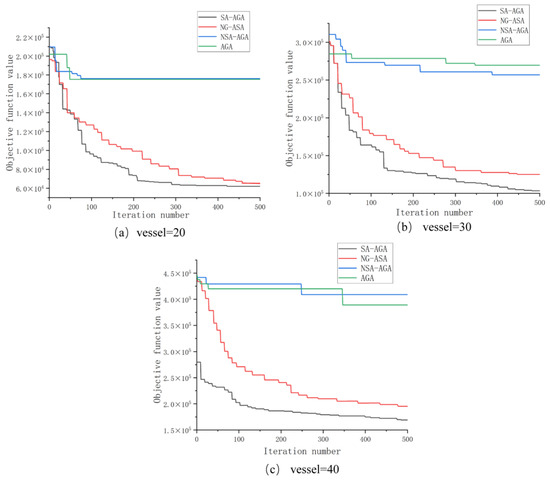
Figure 4.
Comparison of convergence curves of each algorithm.
Furthermore, the curves of SA-AGA and NG-AGA indicate that the use of both the random generation strategy and the greedy construction strategy during population initialization leads to faster convergence of the objective function values with an increasing number of ships to be dispatched, and lower objective function values are obtained. These findings suggest that the proposed SA-AGA algorithm has better performance compared to the other algorithms tested.
5. Numerical Experiments
This paper presents numerical experiments to validate the algorithm proposed in Section 4. The experiments were conducted on a computer system equipped with an Intel Core i5-8300H CPU clocked at 2.30 GHz and 16 GB of RAM, using MATLAB 2016a as the software platform.
5.1. Parameter Design
Before starting the experiments, it is necessary to determine the parameters. The parameters involved in our experiments can be divided into three categories: terminal parameters, vessel parameters, and algorithm parameters.
5.1.1. Terminal Parameters Design
In this paper, our experimental subject is a port with three container terminals. The lengths of terminals are 1000 [m], 1140 [m], and 1200 [m] respectively; the water depth of quays are 10 [m], 11 [m], and 14 [m] respectively; and the number of quay cranes in each terminal is 11, 12, and 13 respectively. At the same time, as the operational efficiency of quay cranes is uncertain, we set its expected value to [TEU/h] and assume that the actual operational efficiency of the quay cranes follows a normal distribution of . Furthermore, the interference coefficient between the quay cranes is 0.9.
To calculate the objective function value, it is necessary to determine the various cost factors in the port. Table 6 indicates the transshipment cost between terminals for a container. The operating cost for each quay crane is 4.34 per hour. The carbon emissions cost when the vessel’s berthing position is different from the desired berthing position is 0.01 per dollar per meter. The waiting cost for a vessel at anchor is 33.2 per hour. The penalty cost per hour when a vessel departs the port with a delay is 10% of the length . When one ship arrives late, the berthing and departure of subsequent vessels may be affected. Therefore, a penalty cost is needed and we set it to 100 per hour. In addition, the size of the samples is 20.
Table 6.
Transshipment costs between terminals for a container.
5.1.2. Vessel Parameters Design
At the beginning of the scheduling period, we assume that several vessels have berthed already and are being served.
Table 7 outlines the parameter ranges for both scheduled and unscheduled vessels. The symbol indicates a uniform distribution, while represents the set of integers. The planning period is , and the number of vessels scheduled at each terminal is between 1 and 3. In addition, it is worth noting that the draft constraint should be met when determining the berthing terminal or the pre-assigned terminal of the vessels. The drafts for all vessels are obtained according to (26).
Table 7.
Range of vessel parameters.
5.1.3. Algorithm Parameters Design
Before using the algorithm, the necessary parameters need to be determined. In this paper, we set the population size , the number of generations , and the initial probability . In terms of the simulated annealing mechanism, we set the initial temperature , the cooling rate , and the maximum generation of the simulated annealing mechanism .
5.2. Results and Analysis
First, three scheduling strategies are defined. These strategies include multi-terminal cooperative scheduling under uncertainty (referred to as M + U), multi-terminal independent scheduling under uncertainty (referred to as S + U), and multi-terminal cooperative scheduling under certainty (referred to as M + C). We then compare them in terms of the objective function value (i.e., total cost), vessel departure delay rate, quay utilization, and quay crane utilization.
Under the S + U, the mathematical model can be obtained by adding (27) to the MU-BAQCAP. It limits the actual berthing terminal for each vessel to its pre-assigned terminal. The algorithm is also similar to the SA-AGA, except that the berthing terminals of vessels are fixed to their pre-assigned terminals.
According to Section 5.1, ten cases were constructed for each scale of 20, 30, and 40 vessels, respectively. The average value of the algorithm under five runs is used as the final result for each scheduling strategy.
Table 8 displays the objective function values for each experiment under M + U and S + U, with the difference between them referred to as Gap. It is evident that the total cost of scheduling under S + U is considerably higher than that under M + U, with the difference between them increasing as the number of vessels to be scheduled grows. The increase can be attributed to the efficient sharing of terminal resources as the number of ships increases, enabling them to be berthed on schedule and significantly decreasing waiting, delay, and penalty costs.
Table 8.
Objective function values under M + U and S + U.
Similarly to Table 8, the results of the objective function values for each experiment under M + U and M + C are presented in Table 9. The difference between the objective function values of M + U and M + C is defined as the Gap. Again, we can find that the cost of the scheduling solution obtained under M + U is lower than under M + C. However, the difference between them, which is only about 20%, is not as large as the difference between M + U and S + U which is about 50~80%.
Table 9.
Objective function values under M + U and M + C.
The objective function values for each experiment under different scheduling strategies are presented in Figure 5a–c, corresponding to the scale values of 20, 30, and 40, respectively. Clearly, the variations of the objective function values in the M + U and M + C are much smaller than those in the S + U under all scales. The reason is that the workload of each terminal can be more balanced by sharing resources with others. In contrast, in the independent scheduling strategy, when the number of vessels at a particular terminal is much higher than others, these vessels can only wait at anchor due to the inability to share the resources of other terminals. As a result, the queue waiting on the berth becomes longer and the total cost increases. Therefore, in scheduling operations for dispatched vessels at this container port, the highest priority should be given to addressing the impact of uncertain environmental factors, which can result in cost savings of approximately 40–60% for the port. In addition, there is a need to integrate all terminals and coordinate the scheduling of internal resources, which can yield cost savings of approximately 10–20% for the port.
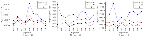
Figure 5.
Objective function values of three scheduling strategies under different scales.
There are many other indicators beyond the total cost that can measure the performance of a scheduling plan in a container port. Therefore, in this paper, three other indicators are selected to further evaluate the scheduling plans obtained under the scheduling strategies: vessel delay departure rate , quay utilization , and quay crane utilization . The vessel delay departure rate is calculated by (28), the quay utilization by (29), and the quay crane utilization by (30).
Here, denotes the number of vessels in sample s that depart later than their desired departure time . indicates the number of vessels to be scheduled. denotes the number of samples; H denotes the planning period. and represent the actual arrival and departure time of vessel in sample s, respectively.
A delay in vessel departure time means that it may not arrive at the next port on time, and thus reduces the satisfaction of the customer. Figure 6 shows the vessel delay departure rates for each experiment in different scheduling strategies under the scales 20, 30, and 40, respectively. As can be seen, in most experiments, the delay rates under M + U and M + C are generally lower than those under S + U. The gap becomes more noticeable as the number of vessels to be scheduled increases, with the difference reaching about 10% in most experiments. Furthermore, the uncertainty factor has little impact on the delayed departure rate, which is slightly higher when considering uncertainties than when not, up to about 8%, but within 5% in most experiments. By adding the buffer time variable, the impact of uncertain factors on the planned berthing time of the ship is taken into account, reducing the possibility of the actual arrival time being later than planned. This implies that the scheduling plan considers uncertainties such as ship arrival time and shore bridge operation efficiency, which can effectively reduce the rate of ship arrival delays, minimizing their impact on subsequent ship berthing and enhancing the plan’s feasibility.
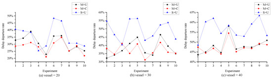
Figure 6.
Vessel delay departure rate of three scheduling strategies under different scales.
Higher utilization of terminal resources means fewer idle resources on the terminal, which also reduces the idle cost. Figure 7 shows the quay utilization in the three scheduling strategies under the scales 20, 30, and 40, respectively. Figure 8 shows the quay crane utilization. From Figure 7a and Figure 8a, it is noted that when the number of vessels to be scheduled is 20, the gap in the quay utilization in different strategies is not significant, so the quay crane utilization is. The reason is that the number of vessels to be scheduled is too small and the resources cannot be fully utilized yet. Therefore, the utilization of resources in different strategies is similar. When the number of vessels to be scheduled reaches 30, the quay and quay crane utilization in the M + U and M + C are still not significant. However, we can still find that the resource utilization under M + C is about 3% lower than under M + U, regardless of the quay or quay crane, as shown in Figure 7b and Figure 8b. As the number of vessels increases to 40, we can find in Figure 7c and Figure 8c that the difference is more significant with resource utilization between S + U, M + C, and M + U, up to about 13% at the maximum. Therefore, as the number of vessels increases, integrating all terminals and coordinating their internal resources can effectively increase the utilization of critical terminal resources.
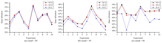
Figure 7.
Quay utilization of three scheduling strategies under different scales.
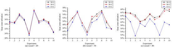
Figure 8.
Quay crane utilization of three scheduling strategies under different scales.
In summary, in the case of a container port with multiple terminals, it can improve the port’s operating cost, the vessel delay, departure rate, and the utilization of quay and quay cranes by sharing their resources and accounting for the uncertainty in vessel arrival time and quay crane operational efficiency.
6. Conclusions and Future Work
The present study investigates the berth allocation problem and quay crane allocation problem for multiple terminals under the context of low carbon emissions and uncertainty in vessel arrival times and quay crane operational efficiency. After considering constraints such as interference between quay cranes, existing berthing vessels at the beginning of the planning period, vessel draft requirements, and container transshipment, a multi-terminal berth and quay crane joint robust scheduling model considering carbon cost (MU-BAQCAP) was developed under the uncertainties. Then, an adaptive improved genetic algorithm (SA-AGA) is designed for the solution in combination with the simulated annealing mechanism, and the applicability of the algorithm is verified through numerical experiments. The results show that, compared with the independent scheduling for multiple terminals under uncertain environments and the collaborative scheduling for multiple terminals under certain environments, scheduling with the uncertain environment and the coordination mechanism for multiple terminals can have a greater advantage in terms of total cost and can more effectively improve the service capacity and competitiveness of container ports. The differences between the results with and without collaborative scheduling are more significant than the ones between the results with or without considering the uncertain environment.
Future research could explore the following areas:
- (1)
- The quay crane allocation problem studied in this paper is static. However, if the quay crane can be used for other vessels before the vessel it is serving departs (dynamic quay crane allocation problem), the utilization of the quay crane can be greatly improved. Therefore, this restriction can be introduced into the model in subsequent research.
- (2)
- This paper assumes that the quay crane can reach anywhere along the quay. However, in the actual operation of a container port, the quay cranes can only move within a fixed area. Therefore, we need to take it into account in future studies to make the model more realistic and feasible.
- (3)
- The scope of this paper is limited to addressing the berth allocation problem and quay crane allocation problem in container port operations. However, there are many other processes involved, such as container truck scheduling, storage allocation, and yard crane scheduling. These processes are interlinked and interdependent. Therefore, more processes need to be included in the study to obtain a more feasible scheduling solution.
Author Contributions
Conceptualization, M.J.; Methodology, G.W.; Software, J.F.; Investigation, Y.Z.; Resources, F.M.; Data curation, J.Z.; Writing—original draft, L.Z.; Project administration, M.J. and F.M.; Funding acquisition, M.J. All authors have read and agreed to the published version of the manuscript.
Funding
This research was funded by National Natural Science Foundation of China, grant number 51605442 and Zhejiang Provincial Natural Science Foundation of China, grant number LGN18G010002.
Institutional Review Board Statement
Not applicable.
Informed Consent Statement
Not applicable.
Data Availability Statement
Data available in a publicly accessible repository that does not issue. DOIs Publicly available datasets were analyzed in this study. This data can be found here: https://github.com/Jiajia-fe/Data-and-Code-for-Article.git, accessed on 12 February 2023.
Conflicts of Interest
The authors declare no conflict of interest.
References
- Frojan, P.; Francisco Correcher, J.; Alvarez-Valdes, R.; Koulouris, G.; Manuel Tamarit, J. The continuous Berth Allocation Problem in a container terminal with multiple quays. Expert Syst. Appl. 2015, 42, 7356–7366. [Google Scholar] [CrossRef]
- Bierwirth, C.; Meisel, F. A survey of berth allocation and quay crane scheduling problems in container terminals. Eur. J. Oper. Res. 2010, 202, 615–627. [Google Scholar] [CrossRef]
- Bierwirth, C.; Meisel, F. A follow-up survey of berth allocation and quay crane scheduling problems in container terminals. Eur. J. Oper. Res. 2015, 244, 675–689. [Google Scholar] [CrossRef]
- De, A.; Pratap, S.; Kumar, A.; Tiwari, M.K. A hybrid dynamic berth allocation planning problem with fuel costs considerations for container terminal port using chemical reaction optimization approach. Ann. Oper. Res. 2020, 290, 783–811. [Google Scholar] [CrossRef]
- Al-Refaie, A.; Abedalqader, H. Optimal berth allocation under regular and emergent vessel arrivals. Proc. Inst. Mech. Eng. Part M-J. Eng. Marit. Environ. 2021, 235, 642–656. [Google Scholar] [CrossRef]
- Wawrzyniak, J.; Drozdowski, M.; Sanlaville, E. Selecting algorithms for large berth allocation problems. Eur. J. Oper. Res. 2020, 283, 844–862. [Google Scholar] [CrossRef]
- Abou Kasm, O.; Diabat, A. Next-generation quay crane scheduling. Transp. Res. Part C-Emerg. Technol. 2020, 114, 694–715. [Google Scholar] [CrossRef]
- Lv, X.; Jin, J.G.; Hu, H. Berth allocation recovery for container transshipment terminals. Marit. Policy Manag. 2020, 47, 558–574. [Google Scholar] [CrossRef]
- Jia, S.; Li, C.-L.; Xu, Z. A simulation optimization method for deep-sea vessel berth planning and feeder arrival scheduling at a container port. Transp. Res. Part B-Methodol. 2020, 142, 174–196. [Google Scholar] [CrossRef]
- Xiang, X.; Liu, C. An expanded robust optimisation approach for the berth allocation problem considering uncertain operation time. Omega-Int. J. Manag. Sci. 2021, 103, 102444. [Google Scholar] [CrossRef]
- Rodrigues, F.; Agra, A. Berth allocation and quay crane assignment/scheduling problem under uncertainty: A survey. Eur. J. Oper. Res. 2022, 303, 501–524. [Google Scholar] [CrossRef]
- Cao, J.; Shi, Q.; Der-Horng, L. Integrated Quay Crane and Yard Truck Schedule Problem in Container Terminals. Tsinghua Sci. Technol. 2010, 15, 467–474. [Google Scholar] [CrossRef]
- Safaei, N.; Bazzazi, M.; Assadi, P. An integrated storage space and berth allocation problem in a container terminal. Int. J. Math. Oper. Res. 2010, 2, 674–693. [Google Scholar] [CrossRef]
- Jonker, T.; Duinkerken, M.B.; Yorke-Smith, N.; de Waal, A.; Negenborn, R.R. Coordinated optimization of equipment operations in a container terminal. Flex. Serv. Manuf. J. 2021, 33, 281–311. [Google Scholar] [CrossRef]
- Agra, A.; Oliveira, M. MIP approaches for the integrated berth allocation and quay crane assignment and scheduling problem. Eur. J. Oper. Res. 2018, 264, 138–148. [Google Scholar] [CrossRef]
- Li, Y.; Chu, F.; Zheng, F.F.; Kacem, I. Integrated berth allocation and quay crane assignment with uncertain maintenance activities. In Proceedings of the International Conference on Industrial Engineering and Systems Management (IESM), Shanghai, China, 25–27 September 2019; pp. 248–253. [Google Scholar]
- Chargui, K.; Zouadi, T.; El Fallahi, A.; Reghioui, M.; Aouam, T. Berth and quay crane allocation and scheduling with worker performance variability and yard truck deployment in container terminals. Transp. Res. Part E-Logist. Transp. Rev. 2021, 154, 102449. [Google Scholar] [CrossRef]
- Ji, B.; Huang, H.; Samson, S.Y. An Enhanced NSGA-II for Solving Berth Allocation and Quay Crane Assignment Problem with Stochastic Arrival Times. IEEE Trans. Intell. Transp. Syst. 2022, 24, 459–473. [Google Scholar] [CrossRef]
- Tang, M.; Ji, B.; Fang, X.; Yu, S.S. Discretization-Strategy-Based Solution for Berth Allocation and Quay Crane Assignment Problem. J. Mar. Sci. Eng. 2022, 10, 495. [Google Scholar] [CrossRef]
- Zhen, L.; Chang, D.-F. A bi-objective model for robust berth allocation scheduling. Comput. Ind. Eng. 2012, 63, 262–273. [Google Scholar] [CrossRef]
- Xiang, X.; Liu, C.; Miao, L. Reactive strategy for discrete berth allocation and quay crane assignment problems under uncertainty. Comput. Ind. Eng. 2018, 126, 196–216. [Google Scholar] [CrossRef]
- Iris, C.; Lam, J.S.L. Recoverable robustness in weekly berth and quay crane planning. Transp. Res. Part B-Methodol. 2019, 122, 365–389. [Google Scholar] [CrossRef]
- Rodrigues, F.; Agra, A. An exact robust approach for the integrate d b erth allocation and quay crane scheduling problem under uncertain arrival times. Eur. J. Oper. Res. 2021, 295, 499–516. [Google Scholar] [CrossRef]
- Prayogo, D.N. Carbon emission modelling in container terminal operations planning using a system dynamics approach. In IOP Conference Series: Materials Science and Engineering; IOP Publishing: Bristol, UK, 2019; Volume 703, p. 012014. [Google Scholar] [CrossRef]
- Sun, Q.; Zhen, L.; Xiao, L.; Tan, Z. Recoverable Robustness Considering Carbon Tax in Weekly Berth and Quay Crane Planning. In Proceedings of the 6th KES Annual International Conference on Smart Education and e-Learning (KES SEEL)/2nd KES International Symposium on Smart Transportation Systems (KES-STS), St. Julian’s, Malta, 17–19 June 2019; pp. 75–84. [Google Scholar]
- Lin, S.; Zhen, L.; Wang, W.; Tan, Z. Green berth and yard space allocation under carbon tax policy in tidal ports. In Maritime Policy & Management; Taylor & Francis: Abingdon, UK, 2022. [Google Scholar] [CrossRef]
- Karam, A.; Eltawil, A.; Reinau, K.H. Energy-Efficient and Integrated Allocation of Berths, Quay Cranes, and Internal Trucks in Container Terminals. Sustainability 2020, 12, 3202. [Google Scholar] [CrossRef]
- Imai, A.; Nishimura, E.; Papadimitriou, S. Berthing ships at a multi-user container terminal with a limited quay capacity. Transp. Res. Part E-Logist. Transp. Rev. 2008, 44, 136–151. [Google Scholar] [CrossRef]
- Krimi, I.; Benmansour, R.; El Cadi, A.A.; Deshayes, L.; Duvivier, D.; Elhachemi, N. A rolling horizon approach for the integrated multi-quays berth allocation and crane assignment problem for bulk ports. Int. J. Ind. Eng. Comput. 2019, 10, 577–591. [Google Scholar] [CrossRef]
- Bouzekri, H.; Alpan, G.; Giard, V. Integrated Laycan and Berth Allocation and time-invariant Quay Crane Assignment Problem in tidal ports with multiple quays. Eur. J. Oper. Res. 2021, 293, 892–909. [Google Scholar] [CrossRef]
- Martin-Iradi, B.; Pacino, D.; Ropke, S. The Multiport Berth Allocation Problem with Speed Optimization: Exact Methods and a Cooperative Game Analysis. Transp. Sci. 2022, 56, 972–999. [Google Scholar] [CrossRef]
- Jiang, M.; Zhou, J.; Feng, J.; Zhou, L.; Ma, F.; Wu, G. Integrated Berth and Crane Scheduling Problem Considering Crane Coverage in Multi-Terminal Tidal Ports under Uncertainty. J. Mar. Sci. Eng. 2022, 10, 506. [Google Scholar] [CrossRef]
- Han, X.-L.; Lu, Z.-Q.; Xi, L.-F. A proactive approach for simultaneous berth and quay crane scheduling problem with stochastic arrival and handling time. Eur. J. Oper. Res. 2010, 207, 1327–1340. [Google Scholar] [CrossRef]
- Beasley, J.E.; Chu, P.C. A genetic algorithm for the set covering problem. Eur. J. Oper. Res. 1996, 94, 392–404. [Google Scholar] [CrossRef]


Disclaimer/Publisher’s Note: The statements, opinions and data contained in all publications are solely those of the individual author(s) and contributor(s) and not of MDPI and/or the editor(s). MDPI and/or the editor(s) disclaim responsibility for any injury to people or property resulting from any ideas, methods, instructions or products referred to in the content. |
© 2023 by the authors. Licensee MDPI, Basel, Switzerland. This article is an open access article distributed under the terms and conditions of the Creative Commons Attribution (CC BY) license (https://creativecommons.org/licenses/by/4.0/).