Article

A Robust Optimization Model for Multi-Period Railway Network Design Problem Considering Economic Aspects and Environmental Impact †

1
Department of Civil Engineering, Science and Research Branch, Islamic Azad University, Tehran 14778-93855, Iran
2
School of Railway Engineering, Iran University of Science and Technology, Tehran 16846-13114, Iran
3
Department of Roads and Transportation, Payame Noor University, Tehran 19556-43183, Iran
*
Author to whom correspondence should be addressed.
This article is taken from a doctoral dissertation by Morteza Noruzi with the title of Development of a model for prioritizing railway development projects based on effective indicators with the guidance of Ali Naderan and the advice of Jabbar Ali Zakeri and Kamran Rahimov in Department of Civil Engineering, Science and Research Branch, Islamic Azad University, Tehran, Iran.
Sustainability 2023, 15(6), 5022; https://doi.org/10.3390/su15065022
Submission received: 9 February 2023 / Revised: 8 March 2023 / Accepted: 9 March 2023 / Published: 12 March 2023

Abstract

:
The railway network design problem is one of the critical issues in the transportation sector due to its significance and variety of necessary applications. The major issue of this field relates to the decision of whether to increase the railways’ capacity or construct a new route to meet demand. Although the budget is a great concern of the managers for making such a decision, environmental factors should be necessarily included in the decision-making process. Therefore, this research proposes a novel robust bi-objective mixed-integer linear programming (MILP) model to simultaneously minimize the total cost and environmental impact under uncertain conditions and within a given time horizon. The proposed problem addresses strategic and operational decisions through railway project selection and product flow determination. To deal with the bi-objectiveness of the model and tackle the complexity of the problem, a nondominated sorting genetic algorithm (NSGA-II) is employed. The proposed NSGA-II could reach near-optimal Pareto solutions in a reasonable solution time and showed a reliable performance for being employed in large-sized instances. It also indicates that the proposed NSGA-II can be utilized for solving large-sized samples in a very short time.

1. Introduction

Railway projects are considered as one of the major construction projects in the countries and require high executive expenses such that construction costs are now a large part of the total construction credits of various countries. Railway transport is considered to belong among the modes of transport with the lowest negative impact on the environment and society [1]. The European Union (EU) has set a target objective of a modal shift from road freight transport towards other more sustainable transport modes of 30% by 2030 and at least 50% by 2050 for shipments over 300 km [1].
Rail freight transportation plays a critical role in the world’s economy and is an indisputable part of transportation in modern society. Duly, investment in the development or construction of a railway network, which comprises the selection of a series of stations along with the links joining them, is affirmed through the resulting savings in energy, time, and pollution emitted by trains. It is also regarded as a firm step towards sustainable development [2]. Therefore, properly selecting railway plans helps to properly plan the transportation sector and the correct orientation in the country’s development, increases the effectiveness of railway networks, and maximizes social and financial benefits. The railway planning problem can be divided into six subgroups: (i) railway network design problem (RNDP), (ii) crew scheduling problem, (iii) rolling stock assignment, (iv) train routing problem, (v) timetabling problem [3], and (vi) line planning problem [4].
However, there are also some challenges and questions to be addressed. The main challenge is the provision of the resources required to improve the current lines or build new lines. Moreover, pollution reduction is another important challenge which needs to be considered continuously. Therefore, the main question is how we can develop a mathematical model and solution method to consider real-world assumptions and find an optimal solution accordingly. Therefore, in this research, a multi-period railway network design problem is studied considering the economic aspects and robustness of the problem. The main goal is to minimize the total cost of designing the rail transportation network from the government’s point of view. Therefore, we consider various economic aspects of the problem, including direct/indirect costs and operating and construction costs, which must be addressed in many studies. On the other hand, the amount of greenhouse gas emissions associated with rail transport is another factor that has received less attention despite recent environmental laws and concerns [5]. To define the problem space, a set of parameters such as network line capacity [6], which plays a very key role in managing network transport demand, is considered. Moreover, double-track and single-track lines are analyzed independently. Another important issue is the budget available to operate the design project, which is spent on building new lines, improving existing lines, and maintenance. All these significantly impact the capacity parameter, and all of which are considered in the form of a category called capacity improvement projects. On the other hand, to make the model closer to real-world conditions, the cost of lost demand is also assumed, which plays a decisive role in determining the optimal values of the variables and the total cost. Finally, the most critical issue is to consider the degree of uncertainty of the demand parameter in the network, which is formulated based on the interval uncertainty and the proposed linear programming by [7]. Since demand is inherently uncertain, and based on the available information, the uncertainty of the interval in the form of defining the lower and upper bounds in an interval is the best way to deal with it; therefore, the robust optimization approach is employed, which has high efficiency in dealing with uncertainty.
The remainder of this paper is structured as follows. Section 2 reviews the relevant background of the discussed problem. Section 3 presents the problem assumptions and the proposed mathematical modelling of the problem. Section 4 describes the robust approach, and the problem’s robust counterpart is developed. The applied solution methods are discussed in Section 5. In Section 6, the parameter adjustment of the algorithm is investigated. The results and a discussion of the proposed algorithms are presented in Section 7. Finally, the conclusion is given in Section 8.

2. Background

This section reviews the studies related to the railway network design problem (RNDP). In an early study. In an early study [8], the authors indicated that railway projects could be completed in different phases, either gradually or all at once. To solve the problem, they employed a heuristic time sequence method. They also reduced the model size significantly by ignoring the small demands from the origin–destination (OD) matrix and preloading them onto their shortest path. This size reduction had little effect on the optimality level of the problem. Lin et al. [9] studied a railway network design problem, considering the project budget and routing costs. In their model, decisions such as establishing a new railway or extending the old railways were made. Yan et al. [10] extended the railway network design model in multiple stages. They also investigated the effects of investment on the railway project choice.
Arnold et al. [11] developed a mixed-integer linear programming model which aimed to determine the optimal location of rail terminals. They employed a heuristic approach to solve their model. Pazour et al. [12] designed a network model for high-speed railways and highways to reduce road congestion. The model objective was the minimization of travel time, and the model was uncapacitated. Sun et al. [13] developed a bi-level programming model for a transport network by considering multi-periods and demand uncertainty in the model. The model was able to optimize the form of the transport network and the construction time at the same time.
Laporte et al. [14] designed a railway network considering the network robustness. The study focused on designing railway lines so that the utility function is optimized. Marín and García-Ródenas [15] developed a model for rapid transit networks which aimed to maximize the transit demand and minimize the travel time. They also considered budget constraints and limitations for the physical networks. In another study, they studied an integrated model of network design and line planning without decreasing the system efficiency in the case of zero failure [16]. They solved the problem by considering the concept of robustness from users’ and operators’ viewpoints.
In the context of rapid transit network design, a Simulated Annealing (SA) algorithm was utilized to maximize trip coverage in the problem [17]. Garcia et al. [18] designed an infrastructure railway network and developed a robust model of the problem as well. They employed a greedy randomized adaptive search method for solving their problem. Canca et al. [19] presented a railway rapid transit network design in line with line planning. They considered and minimized the total cost, including construction costs, fleet purchase costs, train operational costs, and personnel costs. Syedvakili et al. [4] developed a mixed-integer model for designing a railway network from the government’s viewpoint. The model made decisions such as constructing a new line or improving the existing line, and the objective function was to minimize the total costs. A joint multi-objective, decision-making model for the capacity optimization and allocation of an urban railway network was offered by Wang et al. [20] using multi-source data. They applied their proposed methodology to the Beijing metro system, considering the operational costs of trains and the costs related to the waiting time of passengers. Seyedvakili et al. [21] proposed a multi-period railway network design model for the long-term planning of the railway network. Using multi-period railway network design problems can help decisionmakers consider various development projects, even when constructing new lines and improving existing lines.
Many countries are currently seeking effective methods to reduce carbon emissions. The transportation industry plays a significant role among the sources of air pollution. Lin et al. [22] analyzed the carbon emissions of railway and highway transport, estimated the environmental benefit of building a railway, and recommended that the railway network design be modeled as a bi-level programming problem, considering emissions.
In terms of a solution method, many studies have employed multi-objective metaheuristics to solve the problem by generating Pareto frontiers [23,24,25].
Considering the literature, we define our main contributions as follows:
  • The possibility of expanding the existing capacity of the rail transport network through construction projects;
  • Considering demand shortage and time horizon in the problem;
  • Considering greenhouse gas emissions as a result of rail transportation operations and minimizing the total emissions in line with the total costs;
  • Studying the uncertainty of demand using the robust optimization approach;
  • Solving the problem bi-objectively using exact and meta-heuristic approaches.

3. Problem Definition

3.1. Problem Assumptions

The main assumptions of the problem are: (i) a set of new or existing directed arcs is considered in the network, (ii) the budget is limited, (iii) a planning period (time horizon) is defined, (iv) each arc or rail line has a limited capacity, (v) the capacity of any existing arc or rail line can be increased by defining a new project at the beginning of the time horizon, (vi) each project has a cost that is calculated based on the available budget, (vii) lost demand is considered in the problem, and (viii) the rail freight demand between each pair of origin–destination nodes (OD) is uncertain.

3.2. Mathematical Modelling

The proposed model investigates the effects of two important factors, including planning period and pollution reduction, which have not been addressed previously. The mathematical modelling for the proposed railway network design problem is presented as follows:
Sets
A Set of directed arcs (rail lines),                
A Set of new directed arcs (rail lines),                
K Set of origin–destination (OD) pairs,                
P Set of capacity improvement projects,                
T Set of time periods.                
Parameters
B The available budget for projects,
C A P i j The capacity of arc ( i , j ) ,
C A P i j t p The added capacity to the arc ( i , j ) as a result of project p at period t ,
C C p Fixed cost of conducting project p ,
C O i j t The unit operational cost for arc ( i , j ) at period t ,
G H G i j The amount of greenhouse emissions on the arc ( i , j ) ,
C U t o d The cost of lost demand for each pair of ODs at period t ,
D t o d The demand between each pair of ODs at period t ,
δ i j p 1 if arc ( i , j ) belongs to the project p, otherwise 0.
Decision variable
u d t o d Lost demand for each pair of ODs at period t ,            
x i j t o d The flow of each OD in arc ( i , j ) at period t ,            
y p 1 if project p is conducted, otherwise 0.            
Regarding the sets, parameters, and variables, the proposed mathematical modelling is defined.
minimize   T C = t T o d K ( i , j ) A A C O i j t x i j t o d + t T o d K C U t o d u d t o d
minimize   G H G = t T o d K ( i , j ) A A G H G i j   x i j t o d
Subject to
p P C C p y p B ,
j x i j t o d j x j i t o d = D t o d u d t o d i = o ; o d K ; t T ,
j x j i t o d j x i j t o d = D t o d u d t o d i = d ; o d K ; t T ,
j x i j t o d j x j i t o d = 0 i o d ; o d K ; t T ,
o d K x i j t o d C A P i j + p P C A P i j t p δ i j p y p i , j A A ; t T ,
x i j t o d , u d t o d 0 o d K ; t T ,
y p 0,1 p P .
Objective Formula (1) includes minimizing the total cost of the network (transportation costs and lost demand). Objective Formula (2) seeks to minimize the total volume of greenhouse gas emissions in the rail transport network. Constraint (3) expresses the budget limitation for the total cost of the projects. This budget covers all types of budgets needed for capacity improvement projects. Constraints (4) to (6) define the network equilibrium relationships that transfer demand from origins to destinations, considering the possibility of losing the demand in each period. Constraint (7) indicates the capacity constraint that prevents the high flow in the arcs (railway blocks) and increases capacity by carrying out projects on the arcs. The effect of increased capacity is incorporated in a given time period. Constraints (8) and (9) show the domain of the variables. The presented model is deterministic, while traffic demand is an uncertain parameter. Hence, an approach based on robust optimization is presented in the next section to address the inherent uncertainties.

4. Robust Counterpart of the Mathematical Model

Robust optimization searches for near-optimal solutions which are feasible with high probability [26]. Moreover, it proposes a linear formulation that contributes to the suggested mixed-integer linear programming (MILP) of the problem, which is usually neglected by other techniques such as stochastic programming. Hence, in this research, the model proposed by [7] is further explained for the linear optimization problem, in which the objective function is minimized and the uncertainty coefficients exist in both the objective function and the constraints.
The optimization problem is assumed as follows:
minimize   c T x subject   to A x b l x u
Moreover, the uncertainty level is defined as:
The constraint coefficient a i j , j N = 1,2 , , n is modelled as an independent random variable that is symmetrical; however, a ^ i j , j N are of unknown distribution. They take value in the interval [ a i j a ^ i j , a i j + a ^ i j ], where a ^ i j indicates the deviation from the nominal coefficient a i j . Similarly, the objective coefficients c j , j N assume the value in the interval of [ c j d j , c j + d j ], where d j is the deviation from the nominal coefficient c j . Since the objective function is minimization and the purpose of robust models is to obtain the maximum regret, only one side of the proposed interval is considered. Accordingly, it is supposed that c j takes value in [ c j , c j + d j ].
Now, Γ i is defined as below to formulate the robust counterpart:
Let constraint i be as a i T x b i . J i is denoted as a set of uncertain coefficients in row i. For each row of i, a parameter of Γ i (it is not necessarily an integer number) is defined such that [ 0 , J i ] . In fact, the role of Γ i in constraints is to justify the suggested approach’s robustness and the solution’s conservatism level. It has been proven that all coefficients are unlikely to become uncertain simultaneously [7]. Therefore, it can change to the maximum value of [ Γ i Γ i ] a i t . In other words, only a subset of coefficients is allowed to affect the solutions adversely. This assumption ensures that, if the same condition occurs, the optimally robust solution will be feasible. Furthermore, due to the symmetric distribution of the variables, even if the number of changing coefficients violates Γ i , the optimal solution will remain feasible with a very high probability. Hence, Γ i is considered as the protection level for constraint i. Γ 0 controls the robustness level in the objective function. Therefore, it is intended to determine the optimal solutions when Γ 0 number of coefficients are changed in the objective function and have the greatest impact on the solution. Generally, higher values of Γ 0 raise the conservatism level against the higher cost it should be paid in the objective function. Γ 0 is necessarily an integer number; however, the rest of Γ i s can be an integer or non-integer. On this basis, the nominal linear robust counterpart of the problem is obtained as follows [7]:
minimize c T x + max s 0 | s 0 J 0 , s 0 Γ 0 j s 0 d j x j subject   to j a i j x j + max s i t i | s i J i , s i Γ i , t i J i \ s i j s i a ^ i j x j + ( Γ i Γ i ) a ^ i t i x t i b i , l x u ,
To transform the model into a linear optimization model, Lemma 1 is needed.
Lemma 1.
For the vector  x * ,  the protection level of constraint  i  is calculated through Equation (12):
β i ( x * , Γ i ) = max s i t i | s i J i , s i Γ i , t i J i \ s i j s i a ^ i j x * j + ( Γ i Γ i ) a ^ i t i x * t i ,
which is equal to the optimum value of the objective function of the linear model in Equation (13).
β i x * , Γ i = m a x j J i a ^ i j x * j z i j subject   to j J i z i j Γ i , 0     z i j     1   i , j J i .
Lemma 1 was proved in Bertsimas and Sim (2004). By inserting the dual of Equation (13) in the robust counterpart model, it is formulated as follows:
minimize c T x + z 0 Γ 0 + j J 0 p 0 j   subject   to   j a i j x j + z i Γ i + j J i p i j b i i z 0 + p 0 j d j y j i J 0 , z i + p i j a ^ i j y j i 0 , j J i , p i j 0 i , j J i , y j 0 j , z i 0 i , y j x j y j j , l j x j u j j .
Assume that we have x b = A equation, instead of A x b . Then, the robust model could be gained using the following inequality (Hatefi and Julai, 2014) [27]:
A Γ A ^ x b A + Γ A ^
Therefore, using the demand uncertainty interval D t o d ~ [ D t o d D t o d ^ , D t o d + D t o d ^ ] , the optimal robust optimization model is presented as follows:
minimize   T C = t T o d K ( i , j ) A A C O i j t x i j t o d + t T o d K C U t o d u d t o d
minimize   G H G = t T o d K ( i , j ) A A G H G i j x i j t o d
subject to
D t o d Γ t o d D t o d ^ u d t o d j x i j t o d j x j i t o d D t o d + Γ t o d D t o d ^ u d t o d i = o ; o d K ; t T ,
D t o d Γ t o d D t o d ^ j x j i t o d j x i j t o d D t o d + Γ t o d D t o d ^ u d t o d i = d ; o d K ; t T ,
Equations (3) and (6)–(9).

5. Solution Method

In this section, the methods for solving the robust mathematical model are presented. According to the bi-objectiveness of the model, an Epsilon constraint method is supposed to solve the model optimally. Moreover, a nondominated sorting genetic algorithm (NSGA-II) is employed to solve large-sized problems.

5.1. Exact Method: ε-Constraint (EC)

The ε-constraint (EC) is a popular method to resolve multi-objective problems by generating Pareto frontiers. It considers one of the objectives as the main objective of the problem and transfers the other objective functions into the constraints in each step [28]. The superiority of ε-constraint among other exact methods is its ability to control the number of generated Pareto solutions. In other words, the problem is solved by considering different values of ε i , and a Pareto solution is reported each time. For the proposed problem, the EC method is employed through Model (20):
minimize   f 1 x x X , f 2 x ε 2 , f n x ε n .
The main steps of the EC method are: (i) Selecting an objective as the main objective function of the problem; (ii) The problem is solved in a single-objective mode for each objective function, and the optimal value of each objective function is obtained; (iii) The difference between the maximum and minimum values of the second objective function is divided into several predetermined parts. A table of values ε 2 , , ε n   is then generated; (iv) The problem is solved using the main objective function and ε 2 , , ε n   ; (v) Pareto solutions are reported.

5.2. Metaheuristic Approach: NSGA-II

Metaheuristic algorithms provide computational intelligence paradigms that are particularly used for complex optimization problems [29]. In the literature, NSGA-II is known as one of the most popular and widely employed algorithms used to deal with multi-objective optimization models [30]. Besides the functionality of NSGA-II, it can be considered as a standard for many other multi-objective optimization algorithms. The unique approach of NSGA-II in resolving multi-objective optimization problems has been used repeatedly to create a novel algorithm. Undoubtedly, this algorithm is one of the most basic multi-objective evolutionary optimization algorithms; therefore, it is employed in this research. To represent a viable solution of the proposed NSGA-II, a binary string is defined to show the solution representation. Figure 1 presents the specified string for the NSGA-II algorithm.
The chromosome in Figure 1 contains p cells. A randomly generated number between 0 and 1, which is assigned to each cell: cells with a value below 0.5 change to 0, and those above 0.5 are rounded up to 1. The cells with a value of 1 show that the project related to that cell is conducted. By specifying the conducted projects, the arcs for each project are known. Then, each of these arcs is allocated a flow value randomly between their half of the capacity and their full capacity. Note that the arcs with the lower costs and rate of emission are of high priority when being allocated. Given the conducted projects and arc flows, the lost demand is calculated. All these values together form one initial solution for the NSGA-II algorithm. After generating the initial solutions, they may violate one or more problem constraints. In this case, the algorithm finds a neighborhood solution to satisfy the constraints. Then, a single-point crossover and mutation are implemented on the generated initial solutions to form a new population for the next generation. The pseudo-code of the proposed NSGA-II is presented as below Algorithm 1 [31].
Algorithm 1. Pseudo-code of proposed NSGA-II.
1. Initialize population
2. Generate N random solutions and insert into population
3. For (i=1 to MaxGen) do
4. Generate Childpop of size N
5. Select Parents from Population
6. Create Childern from Parents
7. Mutate Childern
8. Combine Population and ChildPop into CurrentPop whth size 2N
9. FOR each individual in CurrentPop DO
10. Assign rank based on Pareto non-dominated sort
11. End FOR
12. Generate sets of non-dominated vectors along Pareto Front
13. LOOP by adding solutions to next generation of Population starting from the best front
14. UNTIL N solutions found and determine crowding distance among the points of each front
15. End FOR
16. Print results

6. Parameter Adjustment: Taguchi Method

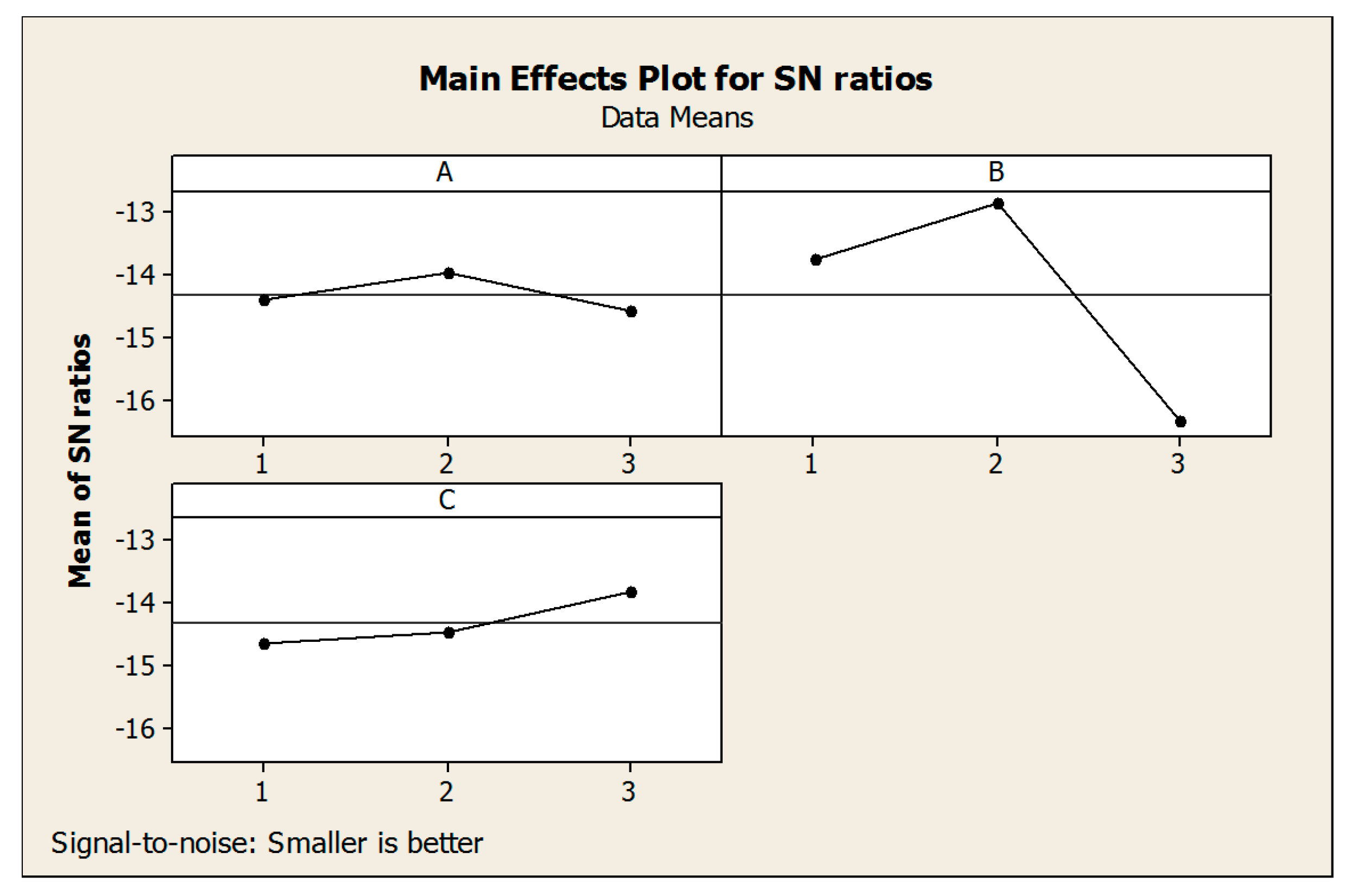
The parameters of the NSGA-II algorithm require an adjustment to attain higher-quality results. For this purpose, the Taguchi method is applied to obtain the optimal value of the NSGA-II parameters. Accordingly, three levels have been considered for each parameter of the NSGA-II given in Table 1. All these different levels solved the problem, and the results were analyzed using MINITAB software. The results of the Taguchi parameter adjustment are shown in Figure 2 and Table 1 and Table 2.

7. Computational Results

In this section, the computational outputs are presented and analyzed. To do so, 15 problem instances are designed in small, medium, and large sizes, which are then solved with the suggested exact method and metaheuristic algorithm. Table 3 and Table 4 illustrate the size of the different problems and value of the parameters, respectively.

7.1. Validation of the NSGA-II

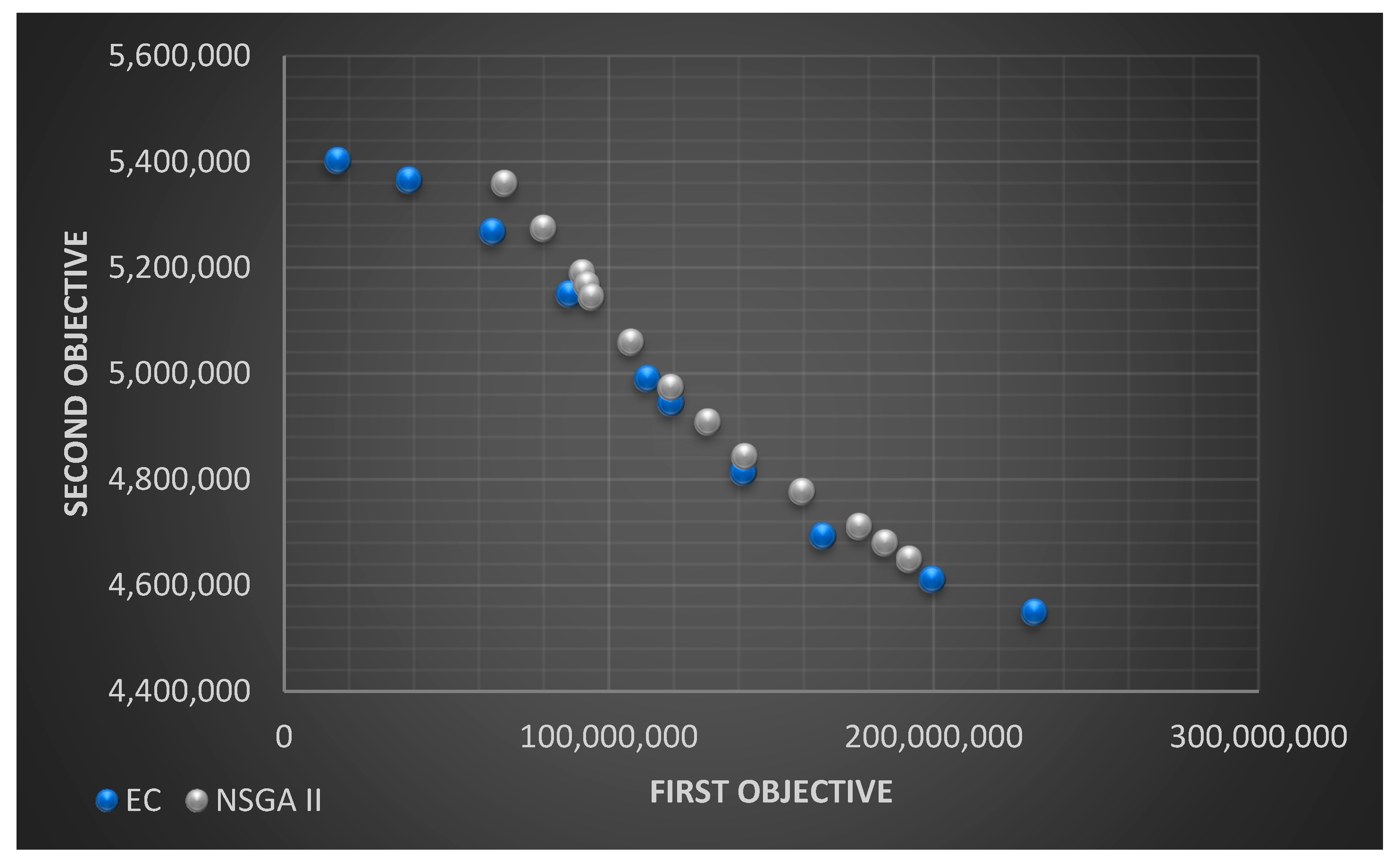
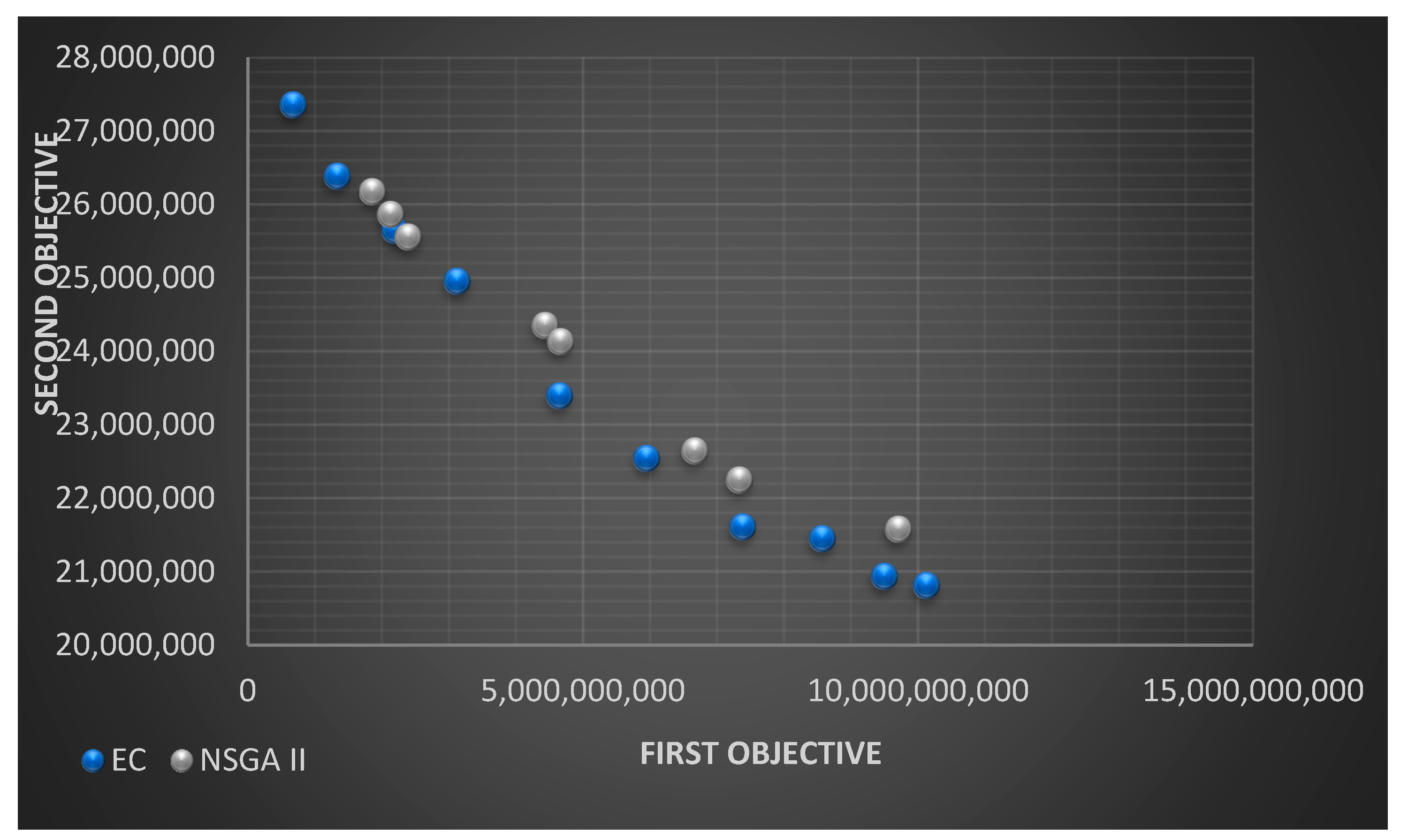
To validate the performance of NSGA-II, the results of the exact method are compared to the algorithm. All these 15 problem instances were solved using ε-constraint (EC), and each problem’s Pareto frontier was extracted. The EC method was implemented in GAMS software using a CPLEX solver with a 3600 s time limitation for implementation. Then, the results of the proposed NSGA-II were compared to the EC, and the performance of the algorithm was evaluated. In larger problems, the EC was not capable of solving the problems optimally in the proposed time limitation. The results of Problems 1 and 6 are displayed as a problem of small- and medium-sized Pareto frontiers. The metaheuristic was coded in MATLAB software and implemented on an operating system Intel® Core™ i7-2600 CPU @ 3.40 GHz, 4.00 GB and 64-bit. Figure 3 and Figure 4 represent the Pareto frontier of Problems 1 and 6, respectively. The figures show the conflict between the model objectives and the trade-off between them. In other words, they have an inverse relationship. The larger the first objective, the lower the second one.
According to Figure 3 and Figure 4, the NSGA-II algorithm generates Pareto frontiers with a negligible gap to the EC. In other words, it is successful in achieving near-optimal solutions and showed a reliable performance.

7.2. Measuring the Performance of NSGA-II

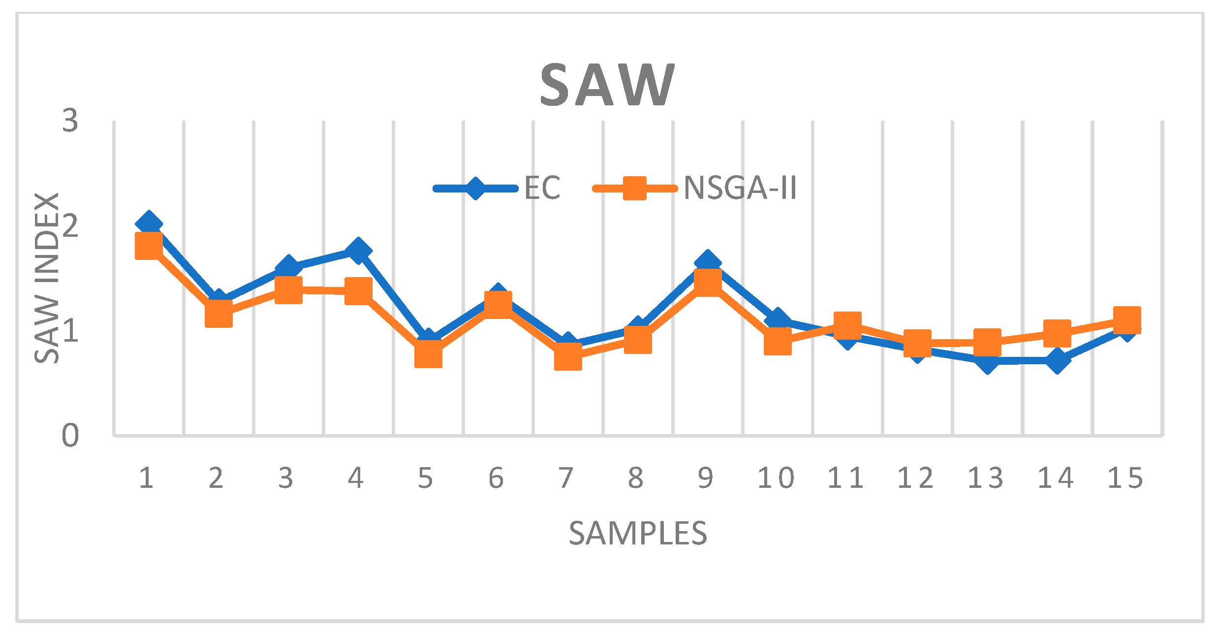
In this section, a number of metrics are used to evaluate the algorithm’s performance with higher accuracy. Mean of ideal distance (MID), space metric (SM), diversification metric (DM), and simple additive weighting (SAW) are defined and calculated for the Pareto frontiers obtained using EC and NSGA-II. Equations (21) to (24) present the formula for MID, SM, DM, and SAW, respectively.
M I D = i = 1 n f 1 i f 1 b e s t f 1 . t o t a l m a x f 1 . t o t a l m i n 2 + f 2 i f 2 b e s t f 2 . t o t a l m a x f 2 . t o t a l m i n 2 n
S M = i = 1 n 1 d d i n 1 d
D M = max f 1 i min f 1 i f 1 . t o t a l m a x f 1 . t o t a l m i n 2 + max f 2 i min f 2 i f 2 . t o t a l m a x f 2 . t o t a l m i n 2
S A W = D M + S M + 1 M I D 3
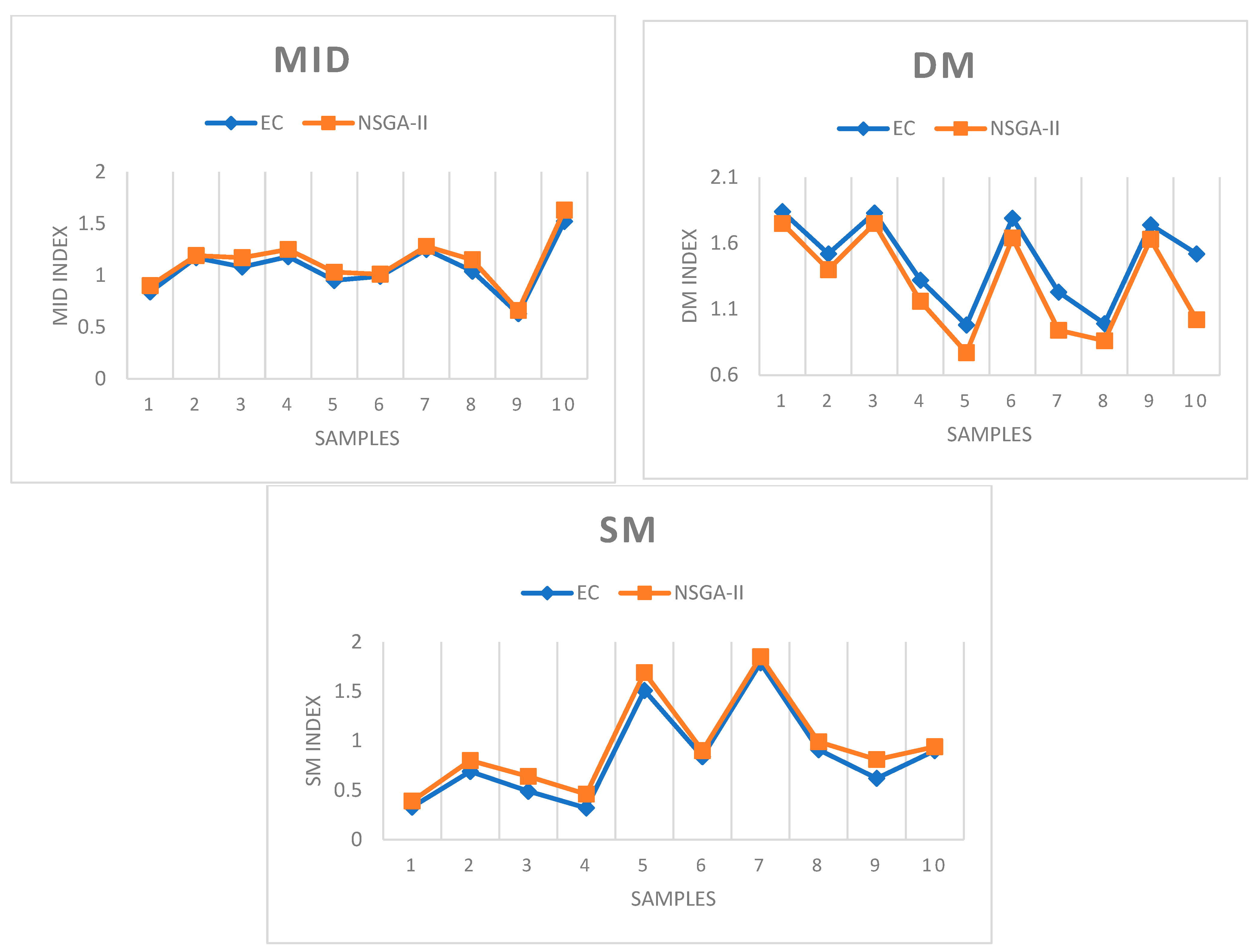
where n is the number of Pareto solutions (i = 1,2, …, n), f i . t o t a l m a x and f i . t o t a l m i n are the maximum and minimum value of objective i in all iterations, ( f 1 b e s t , f 2 b e s t ) is the coordination of the ideal point, d i is the Euclidean distance, and d is the average of d i . Using Equations (21) to (24), the value of the metrics was calculated in each of the 15 problems and is presented in Table 5. In Figure 5, the values of the metrics for small- and medium-sized problems have been compared for both approaches. Accordingly, NSGA-II is rigorous in finding Pareto frontiers close to the optimal frontiers using the EC method. Moreover, for a general analysis of the NSGA-II performance, a comparison of the SAW measure has been presented in Figure 6. This figure also proves the closeness of the Pareto solutions using NSGA-II to the optimal Pareto solutions. As a result, the proposed NSGA-II can be reliable in solving large-sized problems that the EC is not able to solve optimally in the specific time limit.
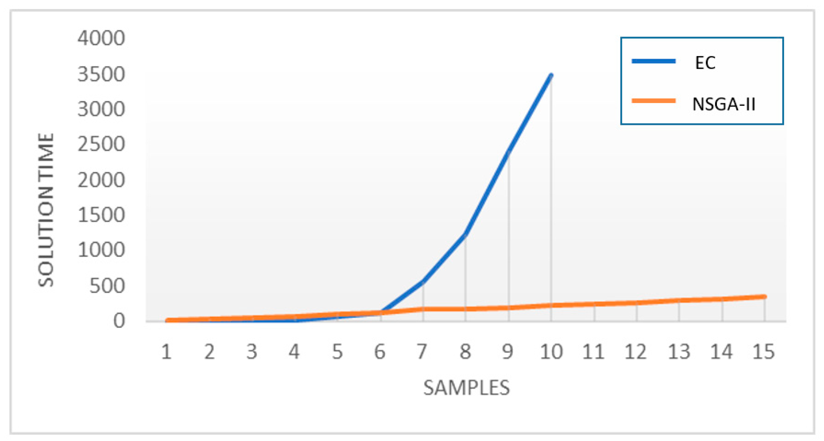
Notably, EC is better than NSGA-II in some cases because it is not capable of solving the problem optimally within the proposed time limit. For instance, in terms of the MID metric, the suggested NSGA-II algorithm shows a better performance than EC when the size of the problem increases. On such an occasion, the proposed NSGA-II can be highly helpful and reliable. Moreover, Table 6 and Figure 7 illustrate the computational time of the methods for each problem. Evidently, by increasing the problem size, the computational time of the EC method increases exponentially, until it cannot solve the large-sized problem in 3600 s. However, the proposed NSGA-II is capable of solving large-sized problems in a reasonable time.

8. Conclusions, Managerial Insights, and Future Works

This paper studied a multi-period railway network design by developing a novel robust bi-objective mixed-integer linear programming (MILP) model. Various economic aspects related to this problem, including direct/indirect costs and operating and construction costs were considered in the model. Moreover, the model was able to lessen the environmental impact. To overcome the demand uncertainty, a robust optimization approach based on interval-based uncertainty was employed. Then, the robust counterpart model of the problem was developed and discussed. The model was solved optimally using the ε-constraint (EC) method. Due to the complexity of the robust model, an efficient metaheuristic, namely, the nondominated sorting genetic algorithm II (NSGA-II), was utilized to deal with large-sized problems. Computational results proved the efficiency of NSGA-II in small- and medium-sized instances as it could find near-optimal Pareto solutions. As a result, the proposed NSGA-II can be utilized for solving large-sized samples in a very short time.
This study could also assist managers and decisionmakers in this area. First, by generating the Pareto frontiers, we illustrated the conflict between cost and emission. This means that the higher amount of cost leads to a lower amount of emission. Here, depending on the viewpoint of the managers, each of the Pareto solutions can be selected as the solution to this problem. If the manager insists on lower expenses, a Pareto solution from the left-hand side of the chart is selected. In the case of being an environmentally friendly manager, a Pareto solution from right-hand side makes more sense. Therefore, it has facilitated the decision making for the managers according to their point of view and policy. Second, the discussion of whether to strengthen the existing facilities or establishing a new one has always been controversial. Based on real data, this study can make such a decision. For instance, a capacity increase is suggested by the model when there are numerous lanes available but cannot fully meet the demand. On the other hand, when there is an insufficient number of facilities compared to the demand, establishing a new lane is recommended.
According to the main limitations of the study, the following suggestions can be considered for future research directions:
  • Developing other uncertainty handling techniques, such as fuzzy programming [32], to be compared to the proposed robust optimization;
  • Applying other well-known algorithms, such as the Multi-Objective Grey Wolf Optimization (MOGWO) algorithm [30] and Multi-objective Particle Swarm Optimization (MOPSO) to be compared to the proposed NSGA-II;
  • Implementing neural networks, machine learning, and deep learning tools to deal with effective demand forecasts [33,34,35];
  • A real case study can be conducted to show the applicability of this model in the real world and provide deeper insights to this problem.

Author Contributions

Methodology, M.N.; Supervision, A.N., J.A.Z. and K.R. All authors have read and agreed to the published version of the manuscript.

Funding

This research received no external funding.

Informed Consent Statement

No applicable.

Data Availability Statement

Not available.

Conflicts of Interest

The authors declare no conflict of interest.

References

  1. Dolinayova, A.; Kanis, J.; Loch, M. Social and economic efficiency of operation dependent and independent traction in rail freight. Procedia Eng. 2016, 134, 187–195. [Google Scholar] [CrossRef] [Green Version]
  2. Aydin, N.S.; Tirkolaee, E.B. A systematic review of aggregate production planning literature with an outlook for sustainability and circularity. Environ. Dev. Sustain. 2022, 1–42. [Google Scholar] [CrossRef]
  3. Zhou, W.; You, X.; Fan, W. A mixed integer linear programming method for simultaneous multi-periodic train timetabling and routing on a high-speed rail network. Sustainability 2020, 12, 1131. [Google Scholar] [CrossRef] [Green Version]
  4. Seyedvakili, S.A.; Nasr Azadani, S.M.; Zakeri, J.A.; Shafahi, Y.; Karimi, M. New model for the railway network design problem. J. Transp. Eng. Part A Syst. 2018, 144, 04018070. [Google Scholar] [CrossRef]
  5. Zeng, Y.; Ran, B.; Zhang, N.; Yang, X. Estimating the Price Elasticity of Train Travel Demand and Its Variation Rules and Application in Energy Used and CO2 Emissions. Sustainability 2021, 13, 475. [Google Scholar] [CrossRef]
  6. Dolinayova, A.; Zitricky, V.; Cerna, L. Decision-making process in the case of insufficient rail capacity. Sustainability 2020, 12, 5023. [Google Scholar] [CrossRef]
  7. Bertsimas, D.; Sim, M. The price of robustness. Oper. Res. 2004, 52, 35–53. [Google Scholar] [CrossRef] [Green Version]
  8. Kuby, M.; Xu, Z.; Xie, X. Railway network design with multiple project stages and time sequencing. J. Geogr. Syst. 2001, 3, 25–47. [Google Scholar] [CrossRef]
  9. Lin, B.; Xu, Z.; Huang, M.; Guo, P. An optimization model to railroad network designing. J. China Railw. Soc. 2002, 24, 1–6. [Google Scholar]
  10. Yan, H.; Lin, B.; Liang, D. An optimization model of railroad network design and investment including multiple projects in several five-year plans. J. China Railw. Soc. 2007, 29, 19–24. [Google Scholar]
  11. Arnold, P.; Peeters, D.; Thomas, I. Modelling a rail/road intermodal transportation system. Transp. Res. Part E Logist. Transp. Rev. 2004, 40, 255–270. [Google Scholar] [CrossRef]
  12. Pazour, J.A.; Meller, R.D.; Pohl, L.M. A model to design a national high-speed rail network for freight distribution. Transp. Res. Part A Policy Pract. 2010, 44, 119–135. [Google Scholar] [CrossRef]
  13. Qiang, S.; Qingyun, W.; Yongling, G. Multi-period bi-level programming model for regional comprehensive transport network design with uncertain demand. J. Transp. Syst. Eng. Inf. Technol. 2011, 11, 111–116. [Google Scholar]
  14. Laporte, G.; Marin, A.; Mesa, J.A.; Perea, F. Designing robust rapid transit networks with alternative routes. J. Adv. Transp. 2011, 45, 54–65. [Google Scholar] [CrossRef] [Green Version]
  15. Marín, Á.; García-Ródenas, R. Location of infrastructure in urban railway networks. Comput. Oper. Res. 2009, 36, 1461–1477. [Google Scholar] [CrossRef]
  16. Marín, Á.; Mesa, J.A.; Perea, F. Integrating robust railway network design and line planning under failures. In Robust and Online Large-Scale Optimization; Models and Techniques for Transportation Systems; Springer: Berlin/Heidelberg, Germany, 2009; pp. 273–292. [Google Scholar]
  17. Kermansshahi, S.; Shafahi, M.; Mollanejad, Y.; Zangui, M. Rapid transit network design using simulated annealing. In Proceedings of the 12th World Conference of Transportation Research, Lisbon, Portugal, 11–15 July 2010; pp. 11–15. [Google Scholar]
  18. García-Archilla, B.; Lozano, A.J.; Mesa, J.A.; Perea, F. GRASP algorithms for the robust railway network design problem. J. Heuristics 2013, 19, 399–422. [Google Scholar] [CrossRef] [Green Version]
  19. Canca, D.; De-Los-Santos, A.; Laporte, G.; Mesa, J.A. An adaptive neighborhood search metaheuristic for the integrated railway rapid transit network design and line planning problem. Comput. Oper. Res. 2017, 78, 1–14. [Google Scholar] [CrossRef]
  20. Wang, B.; Huang, J.; Xu, J. Capacity optimization and allocation of an urban rail transit network based on multi-source data. J. Ambient Intell. Humaniz. Comput. 2019, 10, 373–383. [Google Scholar] [CrossRef]
  21. Alireza Seyedvakili, S.; Zakeri, J.-A.; Nasr Azadani, S.M.; Shafahi, Y. Long-term railway network planning using a multiperiod network design model. J. Transp. Eng. Part A Syst. 2020, 146, 04019054. [Google Scholar] [CrossRef]
  22. Lin, B.; Liu, C.; Wang, H.; Lin, R. Modeling the railway network design problem: A novel approach to considering carbon emissions reduction. Transp. Res. Part D Transp. Environ. 2017, 56, 95–109. [Google Scholar] [CrossRef]
  23. Tirkolaee, E.B.; Goli, A.; Weber, G.-W.; Szwedzka, K. A novel formulation for the sustainable periodic waste collection arc-routing problem: A hybrid multi-objective optimization algorithm. In Logistics Operations and Management for Recycling and Reuse; Springer: Berlin/Heidelberg, Germany, 2020; pp. 77–98. [Google Scholar]
  24. Babaeinesami, A.; Tohidi, H.; Ghasemi, P.; Goodarzian, F.; Tirkolaee, E.B. A closed-loop supply chain configuration considering environmental impacts: A self-adaptive NSGA-II algorithm. Appl. Intell. 2022, 52, 13478–13496. [Google Scholar] [CrossRef]
  25. Ghasemi, P.; Goodarzian, F.; Abraham, A. A new humanitarian relief logistic network for multi-objective optimization under stochastic programming. Appl. Intell. 2022, 52, 13729–13762. [Google Scholar] [CrossRef] [PubMed]
  26. Tirkolaee, E.B.; Goli, A.; Weber, G.-W. A robust two-echelon periodic multi-commodity RFID-Based location routing problem to design petroleum logistics networks: A case study. In Logistics and Supply Chain Management: 7th International Conference, LSCM 2020, Tehran, Iran, 23–24 December 2020; Revised Selected Papers 7; Springer: Cham, Switzerland, 2021; pp. 3–23. [Google Scholar]
  27. Hatefi, S.M.; Jolai, F.; Torabi, S.A.; Tavakkoli-Moghaddam, R. Reliable design of an integrated forward-revere logistics network under uncertainty and facility disruptions: A fuzzy possibilistic programing model. KSCE J. Civ. Eng. 2015, 19, 1117–1128. [Google Scholar] [CrossRef]
  28. Mavrotas, G. Effective implementation of the ε-constraint method in multi-objective mathematical programming problems. Appl. Math. Comput. 2009, 213, 455–465. [Google Scholar] [CrossRef]
  29. Goli, A.; Tirkolaee, E.B.; Weber, G.-W. A perishable product sustainable supply chain network design problem with lead time and customer satisfaction using a hybrid whale-genetic algorithm. In Logistics Operations and Management for Recycling and Reuse; Springer: Berlin/Heidelberg, Germany, 2020; pp. 99–124. [Google Scholar]
  30. Tirkolaee, E.B.; Goli, A.; Ghasemi, P.; Goodarzian, F. Designing a sustainable closed-loop supply chain network of face masks during the COVID-19 pandemic: Pareto-based algorithms. J. Clean. Prod. 2022, 333, 130056. [Google Scholar] [CrossRef]
  31. Hajibabaie, M.; Lotfi, M.M. Fuzzy bi-objective inventory-routing problem for blood products in a hospital network during disasters: Two multi-objective meta-heuristic approaches. Int. J. Logist. Syst. Manag. 2021, 39, 22–51. [Google Scholar] [CrossRef]
  32. Kalantari, H.; Badiee, A.; Dezhboro, A.; Mohammadi, H.; Tirkolaee, E.B. A fuzzy profit maximization model using communities viable leaders for information diffusion in dynamic drivers collaboration networks. IEEE Trans. Fuzzy Syst. 2022, 31, 370–379. [Google Scholar] [CrossRef]
  33. Nguyen, H.; Kieu, L.M.; Wen, T.; Cai, C. Deep learning methods in transportation domain: A review. IET Intell. Transp. Syst. 2018, 12, 998–1004. [Google Scholar] [CrossRef]
  34. Tirkolaee, E.B.; Sadeghi, S.; Mooseloo, F.M.; Vandchali, H.R.; Aeini, S. Application of machine learning in supply chain management: A comprehensive overview of the main areas. Math. Probl. Eng. 2021, 2021, 1476043. [Google Scholar] [CrossRef]
  35. Goli, A.; Tirkolaee, E.B.; Weber, G.-W. An integration of neural network and shuffled frog-leaping algorithm for CNC machining monitoring. Found. Comput. Decis. Sci. 2021, 46, 27–42. [Google Scholar] [CrossRef]
Figure 1. The proposed chromosome for the NSGA-II.
Sustainability 15 05022 g001
Figure 2. Taguchi parameter adjustment for NSGA-II.
Sustainability 15 05022 g002
Figure 3. Pareto frontier obtained using EC and NSGA-II for Problem 1.
Sustainability 15 05022 g003
Figure 4. Pareto frontier obtained using EC and NSGA-II for Problem 6.
Sustainability 15 05022 g004
Figure 5. The comparison of metrics for small- and medium-sized problems.
Sustainability 15 05022 g005
Figure 6. SAW measure for small- and medium-sized problems.
Sustainability 15 05022 g006
Figure 7. Run times for EC and NSGA-II.
Sustainability 15 05022 g007
Table 1. Levels of NSGA-II parameters.
ParameterValue in Each Level
Crossover rate0.6, 0.7, 0.8
Mutation rate0.1, 0.15, 0.2
Initial population200, 300, 400
Table 2. Adjusted optimal values for NSGA-II parameters.
Crossover RateMutation RateInitial Population# of Generation
0.70.1540050
# is nomination for number.
Table 3. Different size instances.
Problem SizeProblem No.# of Directed Arcs# of New Directed Arcs# of Capacity Improvement Projects# of Time Periods
Small15221
26321
37431
48542
510542
Medium612653
713753
815864
9171074
10201284
Large11251595
12301795
135020106
147525106
1510030106
# is nomination for number.
Table 4. Value of parameters.
ParameterDistribution Function ParameterDistribution Function
C A P i j U (1000, 10,000) C U t o d U (100, 300)
C A P i j t p U (100, 1000) D t o d U (10, 150)
C C p U (1000, 5000) δ i j p U (0, 1)
C O i j t U (200, 500) B U (1,000,000, 10,000,000)
G H G i j U (10, 100)--
Table 5. The values of metrics for EC and NSGA-II.
DMMIDSM
ProblemECNSGA-IIECNSGA-IIECNSGA-II
11.841.750.840.90.330.39
21.521.41.171.190.690.8
31.831.751.081.170.490.64
41.321.161.181.250.320.46
50.980.770.951.031.511.69
61.791.640.991.010.840.9
71.230.941.251.281.791.85
80.990.861.041.150.910.99
91.741.630.630.660.620.81
101.521.021.521.630.90.94
111.441.721.451.41.41.39
120.690.731.561.480.880.81
130.851.061.441.111.661.42
140.981.571.981.571.491.4
151.391.480.880.791.831.81
Average1.341.301.201.171.041.09
Table 6. Computational time (s).
Problem123456789101112131415
EC0.24.313.117.266.9112.4549.7123324163491-----
NSGA-II13.529.444.16094.5112.9163.2169.2181.7221.5245.7266.3297.6310.7350.1
Disclaimer/Publisher’s Note: The statements, opinions and data contained in all publications are solely those of the individual author(s) and contributor(s) and not of MDPI and/or the editor(s). MDPI and/or the editor(s) disclaim responsibility for any injury to people or property resulting from any ideas, methods, instructions or products referred to in the content.