Abstract
In order to solve the problems of a slow solving speed and easily falling into the local optimization of an ore-blending process model (of polymetallic multiobjective open-pit mines), an efficient ore-blending scheduling optimization method based on multiagent deep reinforcement learning is proposed. Firstly, according to the actual production situation of the mine, the optimal control model for ore blending was established with the goal of minimizing deviations in ore grade and lithology. Secondly, the open-pit ore-matching problem was transformed into a partially observable Markov decision process, and the ore supply strategy was continuously optimized according to the feedback of the environmental indicators to obtain the optimal decision-making sequence. Thirdly, a multiagent deep reinforcement learning algorithm was introduced, which was trained continuously and modeled the environment to obtain the optimal strategy. Finally, taking a large open-pit metal mine as an example, the trained multiagent depth reinforcement learning algorithm model was verified via experiments, with the optimal training model displayed on the graphical interface. The experimental results show that the ore-blending optimization model constructed is more in line with the actual production requirements of a mine. When compared with the traditional multiobjective optimization algorithm, the efficiency and accuracy of the solution have been greatly improved, and the calculation results can be obtained in real-time.
1. Introduction
1.1. Background and Motivation
Metal mineral resources are nonrenewable strategic materials and represent an important guarantee of national strategic security. There are many poor ores and abundant associated ores in our country, so mineral processing is difficult, and the comprehensive utilization rate is low. With increasingly complex mine production and operation requirements, the previous single-objective plans have been unable to meet the current fine management of multiple minerals in mining enterprises. Therefore, the preparation of a scientific and effective production plan for multimetal and multiobjective open-pit mines will play a vital role in improving the comprehensive utilization rate of the ores, the production cost of the mines, and the economic development of enterprises.
The preparation of an ore-blending plan mainly focuses on modeling and solutions. The modeling mainly takes ore grade, transportation work, production capacity, etc., as the optimization objectives. Single-objective planning mostly adopts 0–1 integer programming, goal programming, and general linear programming methods [1] for modeling. Among them, Wu Lichun et al. [2] adopted a 0–1 integer programming model and embedded it in DIMINE software to study the optimization problem of open-pit mine ore blending with the goal of a balanced quantity of ore. The solving speed and work efficiency of ore blending were significantly improved. Chen Pengneng et al. [3] established a linear programming model with the goal of maximizing the sales value of phosphate rock and solved it with Matlab software. The digital ore-blending model effectively reduced the cost and harmful impurity content. Ke Lihua et al. [4] conducted ore blending for low-grade dolomite and dolomite-grade foreign products and used the ore blending mathematical model to formulate planned ore-blending schemes, which improved the utilization rate of the mineral resources in Wulongquan. Wang Liguan et al. [5] set up an optimization model for open-pit ore-blending with the goal of minimizing grade deviation by using a programming language and created a solver to solve the problem. The algorithm was applied to a copper-molybdenum mine in Inner Mongolia, with strong practical significance. Li Guoqing et al. [6] established a mining operation planning model for underground metal mines based on 0–1 integer programming with the goal of minimizing grade deviation. A computer model and an integer-programming method were used to obtain the optimal scheme for mining operation planning. The ore could be reasonably matched, and the grade could be balanced.
With a demand for increasingly refined production plans, it is necessary to comprehensively consider multiple production indicators, which are often conflicting. Single-objective planning is gradually transitioning to multiobjective planning. In view of the complexity of multiobjective programming models and the difficulty of manual solutions, modern optimization technology can be used to solve the problem. Among them, Yao Xudong et al. [7] used an immune clonal selection algorithm to solve a short-term multiobjective ore matching model of underground metal mines, which could overcome the local optimal situation, and the model could converge stably. Li Zhiguo et al. [8] built a multiobjective ore-blending model for a phosphate ore storage yard with the goal of grinding the flotation raw ore composition index, the stable quality of raw ore, and maximizing the utilization of raw ore and solved this using a multiobjective genetic algorithm. Li Ning et al. [9] established a mine production ore-blending model with ore output and grade fluctuation as the variables and solved it by using a mixed particle swarm optimization algorithm. Gu Qinghua et al. [10] used a genetic algorithm to solve a limestone open pit ore-blending model with the objective function of minimizing grade deviation and the energy consumption of production. Huang Linqi et al. [11] established a metal ore-blending model with grade fluctuation and mining and transportation costs as the output variables and solved it using an adaptive genetic algorithm. Feng Qian et al. [12] used a particle swarm optimization algorithm to solve a sintering-ore-blending model of iron and steel production with the goal of minimizing the cost of blending the materials and maximizing the iron content. Although there are a large number of pieces of research that apply modern optimization methods, such as genetic algorithms, particle swarm optimization, and evolutionary algorithms, to solve multiobjective ore-blending optimization problems, the following challenges still remain. Firstly, most of these algorithms have the problem of a slow convergence speed and easily fall into a local optimum. Secondly, once the environment changes, such algorithms cannot be controlled online and respond quickly and effectively to sudden situations. Finally, most of these algorithms convert multiple objectives into single objectives for a solution and do not fundamentally solve the multiobjective programming problem.
1.2. Research Status
In recent years, with the development of artificial intelligence, machine learning, and other technologies, deep reinforcement learning is gradually becoming favored by researchers. Both reinforcement learning and deep learning are examples of machine learning. Reinforcement learning is an algorithm that constantly interacts with the environment to obtain the optimal strategy. It takes the state as the input and outputs the action strategy. Agents accumulate experience in constant trial and error processes and become more intelligent to make better decisions. From the early single-agent reinforcement learning algorithms, such as the Sarsa [13], Q-learning [14], and DQN [15] algorithms, to today’s multiagent reinforcement learning, reinforcement learning has shown great potential. In recent years, it has gained prominence in areas such as autonomous driving [16], finance [17], and gaming [18]. It has attracted much attention in target detection [19], speech recognition [20], image classification [21], and other fields. Intensive learning pays more attention to decision-making, but its perception of massive data is weak. Deep learning pays more attention to perception but lacks decision-making abilities. Deep intensive learning is an algorithm that combines the perception of deep learning with the decision-making ability of intensive learning. In the face of highly dimensional, complex optimization problems, it can efficiently search and quickly extract features to perceive abstract concepts and optimize strategies through rewards and punishments. Some studies have applied deep reinforcement learning to resource optimization control problems. Deng Zhilong [22] used a deep reinforcement learning algorithm to solve the resource scheduling problem. The deep learning network is trained by using the prior data obtained from the network nodes, and reinforcement learning is used to allocate the network resources. The effectiveness of the algorithm is proved by simulation experiments. Ke Fengkai [23] used a deep deterministic policy gradient algorithm to solve the continuous action control optimization problem. It could realize the fast, automatic positioning of a robot and achieve good results. Xiaomin Liao [24] used a deep reinforcement learning algorithm to solve the resource allocation problem of cellular networks. The proposed algorithm has a fast convergence speed and is obviously superior to other algorithms in the optimization of the transmission rate and system energy consumption. Liu Guannan [25] applied a deep reinforcement learning algorithm to the problem of allocating ambulance resources, and it was superior to the existing algorithms in the indicators of global average response time and initial response rate. Kui Hanbing [26] used deep reinforcement learning to solve the multiobjective control optimization problem of plug-in diesel hybrid electric vehicles, and the proposed algorithm could achieve better control effects. Hu Daner et al. [27] used a deep reinforcement learning algorithm to solve the reactive power optimization control problem of distribution networks. In the face of an unknown environment, it could co-ordinate a variety of reactive power compensation equipment. The simulation results show that the method has low overhead and low delay characteristics.
The above literature shows that deep reinforcement learning has the advantages that traditional optimization control methods do not have when facing highly uncertain optimization decision problems. On the one hand, the algorithm can realize offline training, learn the optimal strategy in the process of continuous trial and error, be controlled online, and obtain calculation results only according to local state information. On the other hand, the algorithm does not rely on an accurate environment model. In the face of unknown environments, agents can achieve real-time decision-making control through local state information. Therefore, using the above ideas, we can apply the deep reinforcement learning algorithm to the multiobjective ore-matching optimization problem of polymetallic open-pit mines. It is unnecessary to establish a complex ore-matching optimization model during training. The agent continuously optimizes the network parameters through the reward and punishment function and finally obtains an optimal ore-matching optimization model. During the test, dynamic ore-blending is realized. The system calculates the action strategy that the agent will take in the next step in real time according to the initial state manually entered, the ore-blending index, and the ore-blending optimization model obtained from training. The agent can respond in real-time even if some unexpected conditions are encountered in the ore-blending scheduling process.
In conclusion, this research proposes a method to solve the optimization problem of multimetal multiobjective ore matching in open-pit mines based on an actor-critic multiagent deep deterministic policy gradient (MADDPG) algorithm [28]. When considering all the indexes of ore grade, lithology, oxidation rate, and ore quantity in the ore-matching scene of an open-pit mine, the ore production sites are regarded as the multiagent with which to co-ordinate control and optimize the ore-matching problem. The time series is discretized, and the interaction process is transformed into the partially observable Markov decision process (POMDP). The agent constantly interacts with the ore-blending environment, learns new strategies through trial and error, and updates the network parameters according to the feedback of the environment so that the agent can get the maximum return. Each agent has two neural networks, namely, the strategic neural network and the evaluation neural network. The strategic neural network obtains control decisions based on local information interacting with the environment, and the evaluation neural network optimizes the strategic neural network based on the global information collected. The MADDPG algorithm is used to train the model, and the training process does not need an accurate optimization model of open-pit ore-blending and does not depend on the prediction data. When compared with traditional multiobjective optimization algorithms, such as the evolutionary algorithm and particle swarm optimization algorithm, which take 3–5 min to calculate each time, in-depth reinforcement learning online co-ordinated optimization can give real-time control strategies based on local state information in 100 milliseconds, which has obvious advantages.
The organizational structure of the paper is as follows: in the first part, the production process of multimetal and multiobject open-pit ore-blending is introduced, and the problem is modeled as a multiobjective optimization problem with the minimum deviation of ore grade and lithology. In the second part, a multimetal and multiobjective ore-matching scheduling algorithm based on multiagent deep reinforcement learning is proposed. In the third part, the simulation experiment is carried out. The simulation scene experimental data parameters and experimental steps are introduced, and the simulation experiment results are obtained. On this basis, the results are analyzed. The fourth part summarizes the work carried out in this paper.
2. Definition and Modeling of Open-Pit Polymetallic Multiobjective Ore-Matching Problem
2.1. Problem Definition
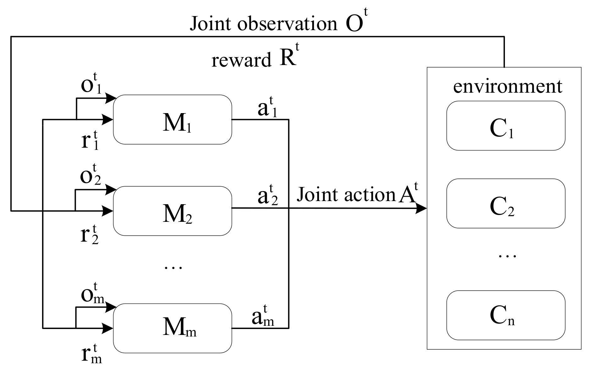
This paper studies the open-pit multimetal and multitarget ore-matching scene, as shown in Figure 1. In the scene, there are m ore production sites and n ore-receiving sites, and the ore production sites are expressed as , and the ore-receiving sites are expressed as . Due to the different ore grades, oxidation rates, lithology, and other parameters of the different ore production sites, the prepared ore-blending plans vary greatly. Each ore production site has b metals, and the grade of each metal is different. The ore supply grades at the ore production sites are expressed as , and the target grades at the ore-receiving sites are expressed as . The ore grade needs to be as close to the target grade as possible under the constraint of minimum grade deviation. The oxidation rate of the ores at each ore production site is different. The oxidation rate of the ores at the ore production sites is expressed as , and the oxidation rate of the ores at the ore-receiving sites cannot exceed the allowable oxidation rate. The ore lithology of each ore production site is different. Grouping and arranging the ore lithology of each ore production site can be expressed as After ore blending, there are various lithologies in each ore-receiving site, and the target lithology ratio is expressed as . The lithology of the ore should be as close to the target lithology as possible under the constraint of minimum lithology deviation. The ore yield of the ore production sites and ore-receiving sites shall meet the requirements of production tasks. See Table 1 for the specific parameters and variable definitions.
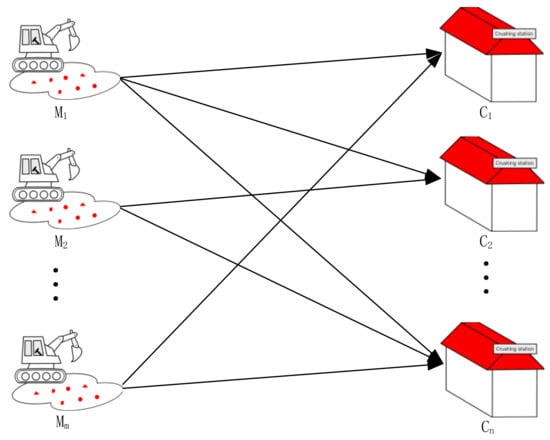
Figure 1.
Schematic Diagram of Ore-Blending Scenarios.

Table 1.
Symbol Description.
2.2. Problem Modeling
2.2.1. Objective Function
The objective function of the multimetal multiobjective ore-blending model of open-pit mines needs to meet the requirements of minimum ore grade deviation and lithology deviation. If the ore-blending task is completed within the planned shift according to the ore-blending plan, the implementation requirements of the planned task will be met; otherwise, the implementation rate of the ore-blending plan will be affected.
(1) The functional expression of ore grade deviation is
(2) The functional expression of ore lithology deviation is
2.2.2. Constraints
Constraint conditions need to comprehensively consider the production capacity of the ore production sites and ore-receiving sites, the oxidation rate constraint, and the deviation of each target quantity.
(1) Constraints on the production capacity of the ore production sites and ore-receiving sites.
When taking into account the ore-matching optimization problem of polymetallic open-pit mines, the production capacity of the excavator at the ore production site needs to consider the actual production requirements. Too much production will lead to the failure of a single operation shift, and too little production will lead to other equipment waiting for a long time, and the crushing capacity of the crushing station at the mining point directly determines the upper and lower limits of the total amount of dynamically circulating ore in the whole environment. In order to ensure that the workload calculated by the ore-blending model is within the capacity range of the ore production and -receiving sites, it is necessary to set a reasonable production capacity constraint range for them.
where Formula (3) represents the constraint condition of the task quantity of ore production site, and Formula (4) represents the constraint condition of the task quantity of the ore-receiving site. and represent the lower limit of the production capacity of the ore production site and ore-receiving site, respectively. and represent the upper limit of the production capacity of the ore production site and ore-receiving site, respectively.
(2) Oxidation rate constraint.
According to the oxidation rate limit index given, the oxidation rate from the ore production site to the ore receiving site is limited.
where represents the upper limit of the oxidation rate of ore at the ore-receiving site.
(3) Constraints on ore grade and lithology deviation.
Considering that the ore grade and lithology need to be as close to the target value as possible, the grade deviation and lithology deviation need to have upper and lower limit constraints:
where Formula (6) represents the constraint condition of ore grade deviation, and Formula (7) represents the constraint condition of ore lithology deviation. and , respectively, represent the lower limit of ore grade and lithology deviation at the ore-receiving site, and and , respectively, represent the upper limit of ore grade and lithology deviation at the ore-receiving site.
3. Multimetal Multiobjective Ore Allocation Algorithm Design for Open-Pit Mine Based on Multiagent Deep Reinforcement Learning
In the multiobjective ore-blending optimization problem of multimetal open-pit mines, the environmental information of the ore-receiving site, such as ore grade, lithology, oxidation rate, and ore amount, changes at every moment. This is a high-dimensional and complex problem with dynamic scheduling over time. Deep reinforcement learning is very good at solving such problems, with its powerful perception and computing ability. Therefore, this study uses a multiagent deep reinforcement learning algorithm to solve this problem.
3.1. Establishment of Multimetal and Multiobjective Ore-blending model in Open-Pit Mines Based on Multiagent Deep Reinforcement Learning
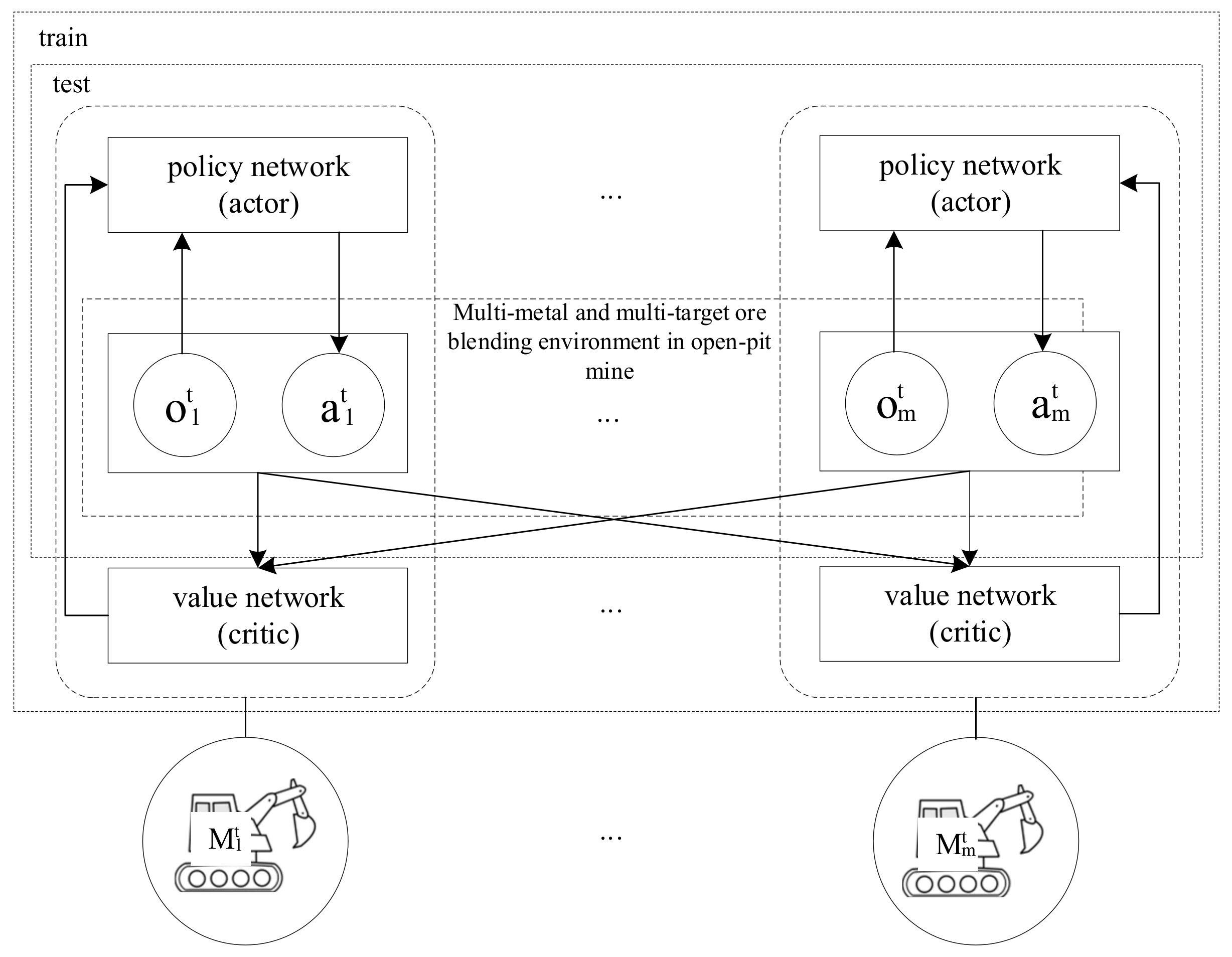
In view of the specific ore-blending scenario of open-pit mines in this study, the ore blending from multiple ore production sites to multiple ore-receiving sites is reasonable to maximize resource utilization. As shown in Figure 2, all ore production sites in the scene are selected as agents; all ore-receiving sites are selected as the environment, and the ore allocation optimization problem is transformed into a partially observable Markov decision-making process. In each time interval, t, each agent takes actions according to the observed state. The environment with the ore-receiving site as the observation object scores the actions taken by the agent and feeds them back to the agent along with the observations while updating the environment. The agents take corresponding actions each time according to the observed value and continuously repeat the above operations, successively deducing the next decision to be made by each agent. According to the objective function and constraint conditions of the multiobjective optimization problem in this scenario, the actions, observations, and rewards of the agent are constructed.

Figure 2.
Agent Real-Time Policy.
(1) Action (A): The action of the agent determines the strategy for ore-blending optimization. When considering the goal of minimizing the deviation of ore grade and lithology by rationally allocating ore resources from the ore production site to the ore-receiving site, at each time, the resource allocation operation from the ore production site to the ore-receiving site in the environment is defined as the action of the agent. The action set of all agents in time period t can be expressed as follows:
(2) Observation (O): This is the process of abstracting the optimization problem of ore distribution into a sequential decision-making problem; that is, the agent needs to make continuous decision-making to achieve the final goal. To facilitate marking the state of an agent, the constraints defined in the previous section are bounded, and the observation set of agent i within the time t can be represented as
In the formula, represents the execution of the task quantity of the ore production site of agent i in the period t. If the executed task satisfies the production capacity constraint of the ore production site defined in Equation (3), is denoted as 1; otherwise, it is denoted as 0. represents the execution of the task quantity of the ore-receiving site of agent i in the period t. If the executed task satisfies the production capacity constraint of the ore-receiving site defined in Equation (4), is denoted as 1; otherwise, it is denoted as 0. represents the optimization of the ore oxidation rate of agent i in time period t. If the current ore oxidation rate of the ore-receiving site is less than the upper limit of the oxidation rate defined by Equation (5), is denoted as 1; otherwise, it is denoted as 0. represents the ore grade optimization of agent i in time period t. If the difference between the target ore grade and the current ore grade at the ore-receiving site satisfies the grade deviation range limited by Equation (6), is denoted as 1; otherwise, it is denoted as 0. represents the lithology optimization of agent i in time period t. If the difference between target lithology and current lithology of ore at the ore-receiving site satisfies the lithology deviation range limited by Equation (7), is denoted as 1; otherwise, it is denoted as 0.
(3) Reward (R): The quality of setting the reward plays a crucial role in the success or failure of the algorithm. The reward in intensive learning can correspond to the constraint conditions in the multiobjective optimization problem. Due to the optimization problem of multimetal and multiobjective ore allocation in open-pit mines, it is necessary to consider the minimum ore grade deviation, minimum oxidation rate, minimum lithology deviation, and ore quantity to meet the production capacity limits of the ore production site and the ore-receiving site. The reward set for agent i can be expressed as
In the formula, represents the reward obtained by agent i in time period t when it meets the production task limit of the ore production site; represents the reward obtained by agent i in time period t when it meets the production task limit of the ore-receiving site; represents the reward obtained by agent i in time period t when it meets the minimum oxidation rate. represents the reward obtained by agent i corresponding to the minimum ore grade deviation in time period t, and represents the reward obtained by agent i corresponding to the minimum lithology deviation in time period t. Therefore, the reward obtained by agent i in time period t is
The total reward for all agents is
3.2. Multiagent Deep Intensive Learning Multimetal Multiobjective Allocation Algorithm in Open-Pit Mines
Traditional reinforcement learning has great advantages in solving single-agent problems, but the effect of the algorithm is greatly reduced when facing a multiagent environment of multimetal and multiple targets in open-pit mining. In the same environment, multiple agents need to co-operate with each other to achieve the final goal, and the stability of the environment needs to be considered. Agents will form their own resource allocation strategies during the learning process. When other agents change their strategies, the environment is usually regarded as unstable. Therefore, we adopted a multiagent deep deterministic policy gradient (MADDPG) algorithm to solve this problem. The main idea of the algorithm was to use centralized training and decentralized execution algorithm architecture. Each agent could make decisions independently and maintain its own network. At the same time, it can obtain information from other agents to better optimize the local value network.
(1) Actor-Critic Network architecture
The Actor-critic architecture of centralized training with decentralized execution includes two kinds of networks, namely a policy-based actor network and a value-based critic network. The actor network can guide the agent on how to choose actions. The critic network is used to evaluate the payoff of the decisions made by the actor network. The actor network updates its parameters in a gradient-descending fashion based on the rewards given by the critic network.
(2) Multiagent deep deterministic policy gradient algorithm
The MADDPG algorithm adopts a dual actor-critic network structure; that is, an evaluation network and a target network. As shown in Figure 3, there are m agents; the policies of all agents are parameterized as , and the set of policies is denoted as . The parameters of the actor policy network in the evaluation network are , and the parameters of the critic value network are . The parameters of the actor policy network in the target network are , and the parameters of the critic value network are . The action-value Q function of the ith agent is the critic network according to the policy π, starting from state O after performing action A; all possible sequences of decisions expected for the reward can be expressed as follows:
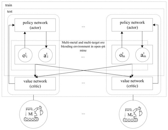
Figure 3.
Architecture of multiagent deep deterministic policy gradient algorithms.
The input of the Q function of the ith agent includes the global information of the states and action values of other agents in addition to its own state and action value, and the obtained Q value can evaluate the action taken by the policy network. By replacing the sum of revenue weighted by the discount coefficient γ received by the agent i in the future into Equation (13), the Bellman equation based on the Q function can be obtained:
Equation (14) describes the iterative relationship between the current state and the future state. Here, represents the immediate reward of agent i, and represents the discounted sum of the future rewards of agent i. The policy network updates the network parameters by minimizing the loss, and the loss function of the ith agent at time t can be expressed as follows:
where H represents H experiences randomly selected from the experience pool; γ is the discount factor, which takes a value between 0 and 1. When γ is smaller, it means that the agent attaches more importance to the immediate benefits, and when γ is larger, it means that the agent attaches more importance to the future benefits. Let μ be the strategy of agent i.
By accessing the local information of its own state, the actor network outputs the action that the agent is about to perform and updates the network parameters by maximizing the policy gradient. The policy gradient of the ith agent at time t can be calculated as follows:
As the parameters of the evaluation network are constantly updated, the parameters of the target network ,, value network, and policy network are updated in a soft update manner:
In the multiagent deep deterministic policy gradient algorithm, the value network guides the policy network to make better decisions by relying on its long-term vision. Once fully trained, the value network is removed for the test time, and the agent is able to make decisions based on the immediate environment using only the policy network. The algorithm architecture can solve two major problems in a multiagent environment: the instability of the environment caused by the change of other agents’ strategies and the cooperation between agents. Through the above analysis, the steps of the open-pit multimetal multiobjective efficient ore-matching scheduling algorithm based on multiagent deep reinforcement learning can be described as follows (Algorithm 1):
| Algorithm 1: Multiobjective efficient ore-blending scheduling algorithm for open-pit mines based on multiagent deep reinforcement learning |
| Initialize MaxEpisode, MaxTime, MaxAgent, and other parameters |
| for i = 0 to MaxEpisode Initialize the open pit multimetal and multiobjective ore-blending environment |
| for j = 0 to MaxTime |
| Based on the environmental input, the ore-blending scheduling instruction is selected for each agent |
| The agent executes the instruction and returns the reward along with the new state of the ore-blending environment |
| The experience of into the experience pool |
| for k=0 to MaxAgent |
| Mini-batch samples are randomly drawn from the experience pool |
| The Q value of the Critic network is calculated according to Equation (14) |
| The network parameters of Critic are updated by minimizing Equation (15) |
| The Actor network parameters are updated by maximizing Equation (16) |
| The Actor target network is updated in a soft update manner according to Equation (17) |
| The target network of Critic is updated in a soft update manner according to Equation (17) |
| end for |
| end for |
| end for |
4. Engineering Application and Result Analysis
4.1. Experimental Data and Parameters
A large open-pit mine in Henan province was taken as the research object, which is rich in molybdenum, tungsten, copper, and other metals. The ore-blending process is often in a relatively difficult state due to the large variety and grade difference of metal produced by each explosion pile. Therefore, this study aimed at bettering the ore-blending optimization process and carried out simulation experiments with the goal of minimizing the deviation of ore grade and lithology, producing a dynamic ore-blending schedule with low deviation and high efficiency over a very short time.
In this study, nine ore production sites and three ore-receiving sites from the mine were selected. As shown in Table 2, the ore-blending parameters of each ore production site include raw ore grade, oxidation rate, lithology, minimum task quantity, maximum task quantity, and other indicators. As shown in Table 3, the ore-blending parameters of each ore-receiving site include target grade, oxidation rate, lithology, minimum and maximum task quantity, and other indicators. The Python3.6 programming language was adopted, and the IDE is Pycharm2019.1.1. With the help of the tensorflow machine learning platform, the computer was configured with Intel Core i5 CPU and 16G memory.
Table 2.
Relevant parameters of ore blending at the ore production site.
Table 3.
Parameters related to ore blending at the ore-receiving site.
4.2. Experimental Steps
The multiagent deep reinforcement learning algorithm described in Algorithm 1 was used for training in the process of multiobjective and multimetal open-pit mine ore-blending optimization. The network parameters were constantly updated, and the final fitting was obtained to determine the ore-blending optimization model. In the experiment, the learning rate was 0.001, the discount factor was 0.95, and the network parameters were updated every 100 training steps for a total of 90,000 training times.
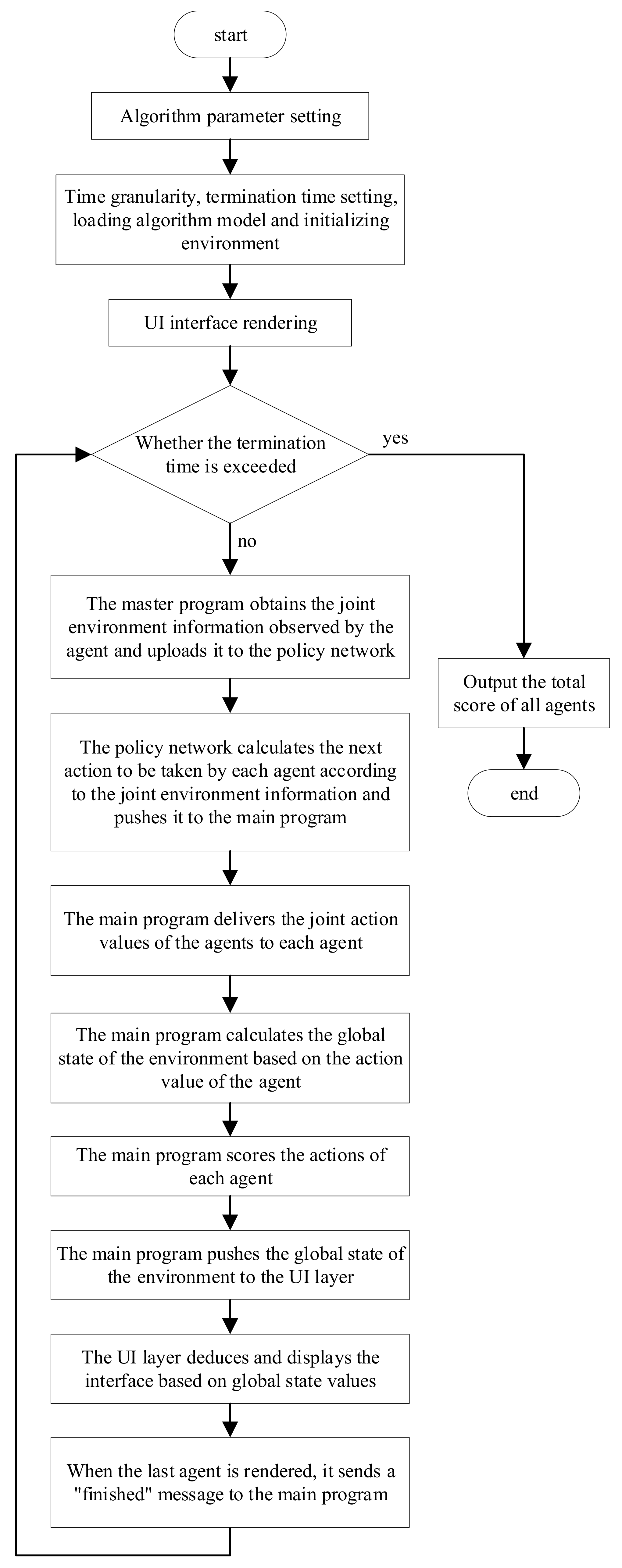
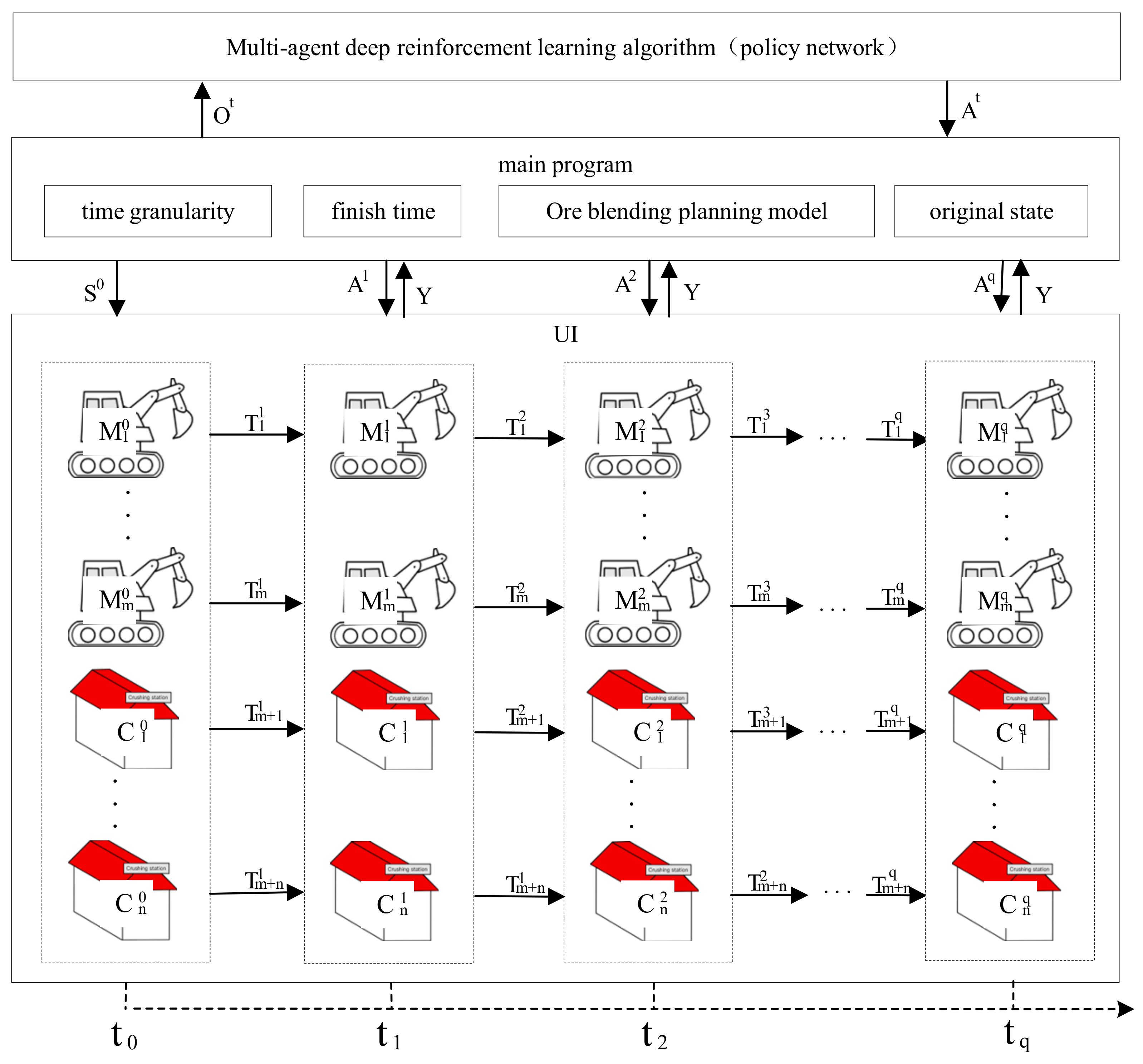
In this section, the simulation experiment method was used to test the above ore-blending optimization model. In the case of known information, such as time granularity, termination time, planning scheme, and the initial state, the artificial system conducts orderly deduction calculations on the behavior and state information of the objects in the application scene with changes in time so as to change the global environment. In the multimetal and multiobjective ore-blending scene of an open-pit mine, the total experimental period is divided into time granularities of equal length. In each calculation cycle, the ore-blending planning model (calculated based on deep reinforcement learning) is simulated. The overall flow chart of the simulation experiment is shown in Figure 4, and the overall architecture is shown in Figure 5, and the specific steps are as follows:
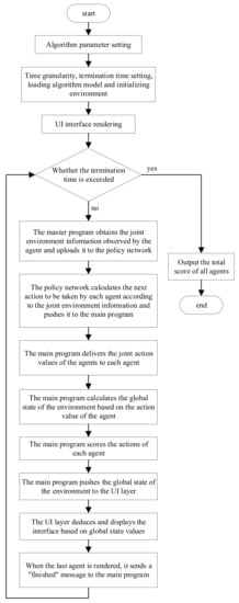
Figure 4.
Flowchart of simulation experiment.

Figure 5.
Overall architecture of simulation experiment.
Step 1: In the initial state, the main program of the ore allocation scheduling experiment extracts the initial state of the global environment from the manually set experimental parameters and pushes it to the UI interface layer. The UI layer renders different objects according to the obtained global environment information and displays them on the window.
Step 2: Each agent in the main program uploads the joint environment information to the multiagent deep reinforcement learning algorithm. The joint environment information consists of two parts: the state information of the agent itself and other agents and the state information of each ore-receiving site in the environment.
Step 3: The algorithm calculates the next joint action of each agent in real-time based on the pushed joint environment information and pushes the joint action command to the main program.
Step 4: First, the main program sends the joint action instructions to each agent and calculates the current state of each ore production site and ore-receiving site in the environment based on the action and the environment state of the previous step. Secondly, the main program scores the degree of influence of the agent action calculated by the algorithm on the environment, where the evaluation index mainly refers to the ore distribution constraints set based on the open-pit polymetallic scene. Finally, the main program pushes the obtained joint environment state to the UI layer.
Step 5: After the UI layer receives the global state information of the environment, the global state of the system is extrapolated forward and displayed on the interface. At this point, a one-hop calculation is completed, and so on until the end of the experiment. In this process, the multiagent deep reinforcement learning algorithm continuously makes sequential decisions to promote the overall environment in a better direction.
4.3. Result Analysis
4.3.1. Analysis of Ore Blending and Scheduling Results
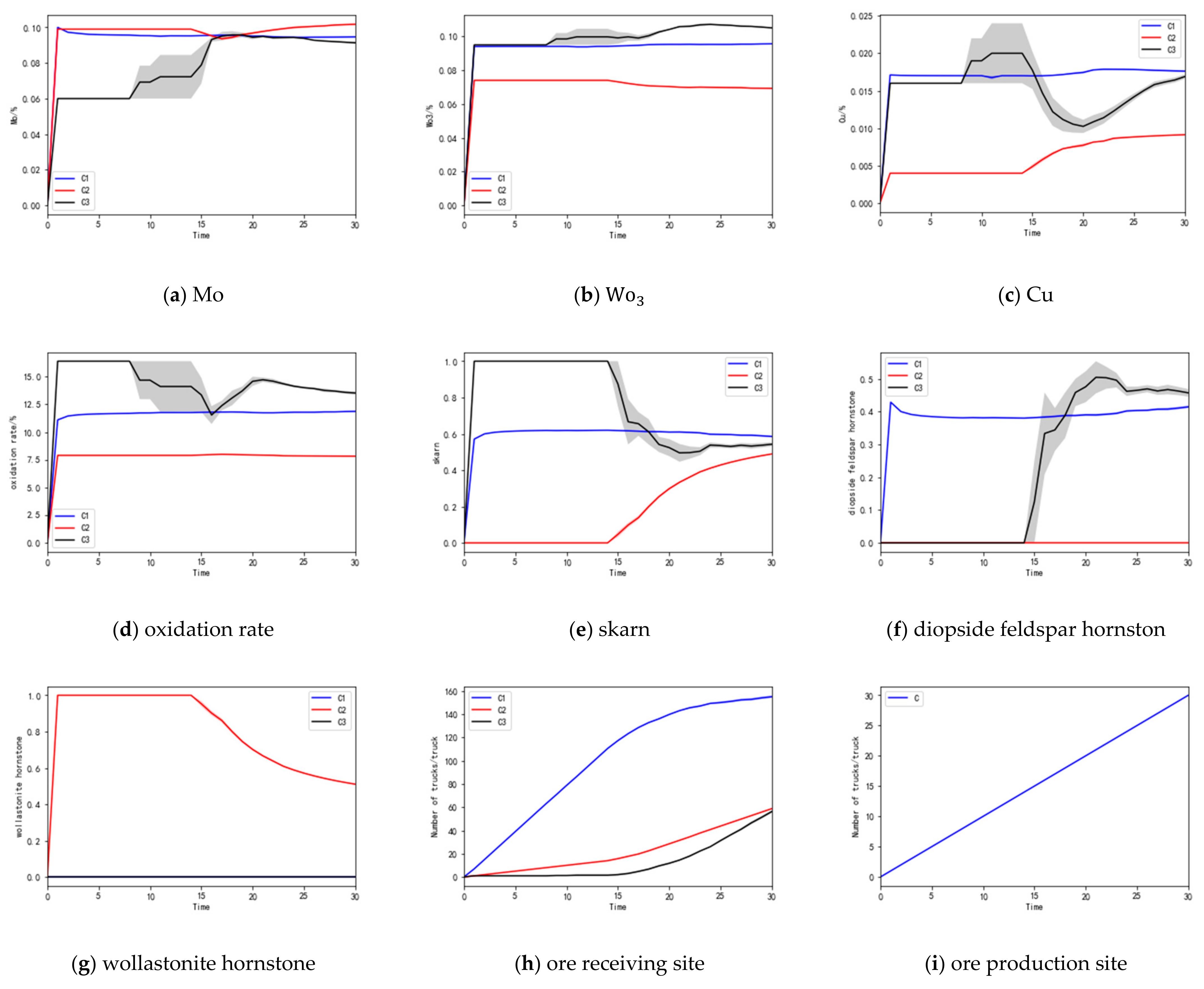
Through the simulation experiments, the trained ore-blending optimization model was tested, and multiple sets of solutions were obtained, which met the open-pit ore-blending optimization model established in Section 1 and achieved the goal of minimizing ore grade deviation and lithology deviation. One group of solutions is presented for analysis, and the obtained ore-blending optimization results are shown in Table 4; the error analysis is shown in Table 5. In the process of the simulation calculations, the change of each index with time is shown in Figure 6a–i, where the horizontal axis represents time. This experiment recorded the mineral supply strategy of the agent at 30 moments; that is, each agent made 30 decisions, and the vertical axis represents the change in each index. The error analysis values in Table 5 were obtained by calculating the difference between the “target value” and the “instantaneous value” of each indicator. The closer the value of the deviation and lithology grades are to zero, the greater the positive deviation of the oxidation rate is, indicating that the ore-blending effect of the algorithm is better.
Table 4.
Ore-blending results of multiagent deep reinforcement learning algorithm.
Table 5.
Error analysis of multiagent deep reinforcement learning algorithms.
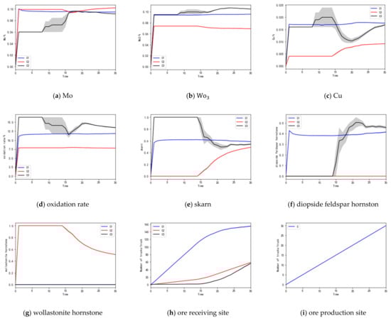
Figure 6.
(a–i) Changes in the indicators of the simulation experiment.
According to the molybdenum metal grade change line chart in Figure 6a, the molybdenum metal grades of , , and at the ore-receiving sites finally stay around 0.095%, 0.101%, and 0.092%, respectively, and the deviation in molybdenum metal grade is controlled within 0.022%. As can be seen from the line chart of tungsten metal grade change in Figure 6b, the tungsten metal grades of , , and at the ore-receiving sites eventually stay at around 0.096%, 0.069%, and 0.105%, respectively, and the deviation in the tungsten metal grades is controlled within 0.008%. As can be seen from the copper grade change line chart in Figure 6c, the copper grades of , and at the ore-receiving sites eventually stay at around 0.018%, 0.009%, and 0.016%, respectively, and the deviation in copper grade is controlled within 0.004%. As can be seen from the oxidation rate variation line chart in Figure 6d, the oxidation rates of , and at the ore-receiving sites eventually stay at around 11.891%, 7.866%, and 13.426%, respectively, and the oxidation rates could reach the minimum value within the allowable error range. As can be seen from the skarn lithology variation line chart in Figure 6e, the skarn lithology of , and of the ore-receiving sites eventually stays around 0.589, 0.483, and 0.537, respectively, and the deviation in skarn lithology is controlled within 0.124. As can be seen from the lithology variation in the diopside feldspar line chart in Figure 6f, diopside feldspar at the ore-receiving sites , , and finally stays around 0.411, 0.000, and 0.463, respectively, and the deviation in diopside feldspar is controlled within 0.036. As can be seen from the wollastonite lithology variation line chart in Figure 6g, the wollastonite lithology of , , and at the ore-receiving sites eventually stays around 0.000, 0.517, and 0.000, respectively, and the deviation in wollastonite lithology is controlled within 0.088. As can be seen from the ore quantity change line chart in Figure 6h, the number of trucks in , , and of ore receiving sites is 158, 58, and 54, respectively, and each truckload is 50 tons, so the ore quantity is 7900, 2900, and 2700 tons, respectively, and the ore quantity at the ore-receiving sites meets the production capacity constraint of the ore-receiving sites. According to the ore quantity change line chart in Figure 6i, it can be seen that the number of cars at each ore production site is finally 30, and the ore quantity is 1500 tons, which meets the production capacity constraint of the ore production site. It can be seen that it is feasible to use the multiagent deep reinforcement learning algorithm to solve the multimetal and multiobjective ore-blending model of open-pit mines, and this has guiding significance for production planning within the allowable range of error.
4.3.2. Comparison of Optimization Methods
(1) Error analysis
In order to verify the solution accuracy of the multiagent deep reinforcement learning algorithm, the deep deterministic policy gradient algorithm was used to compare and analyze it. By applying the multiagent deep reinforcement learning algorithm and deep deterministic policy gradient algorithm to the ore-blending scheduling scene, the performance of solving the optimization problem was analyzed, and the algorithm deviation analysis table shown in Table 6 was obtained. The table shows the deviation changes for each ore index at the collection point under the optimization of the two algorithms. It can be seen from the figure that by using the multiagent deep reinforcement learning (MADDPG) algorithm, the molybdenum metal grade deviation is controlled within 0.022%, the tungsten metal grade deviation is controlled within 0.008%, and the copper metal grade deviation is controlled within 0.004%. The oxidation rate can meet the production requirements within the error tolerance range, and the skarn lithinity deviation is controlled within 0.124. The lithology deviation of the diopside feldspar horn is controlled within 0.036, and that of the wollastonite horn is controlled within 0.088. Using the deep deterministic strategy gradient (DDPG) algorithm to solve the problem, the molybdenum metal grade deviation is controlled within 0.01%, the tungsten metal grade deviation is controlled within 0.019%, the copper metal grade deviation is controlled within 0.006, the oxidation rate is slightly higher than the production requirements, the skarn lithology deviation is controlled within 0.202, and the diopside feldspathite lithology deviation is controlled within 0.296. The lithology deviation of wollastonite horn is controlled within 0.159.
Table 6.
Algorithm deviation.
Through comparative analysis, it can be found that the multiagent deep reinforcement learning algorithm takes 115.708 ms, and the depth deterministic strategy gradient algorithm takes 106.988 ms. When compared with the depth deterministic strategy gradient algorithm, which uses a single agent to optimize the solution, the multiagent deep reinforcement learning algorithm has the same solving efficiency, but the accuracy of the multiagent deep reinforcement learning algorithm has been significantly improved.
(2) Performance analysis of the algorithm
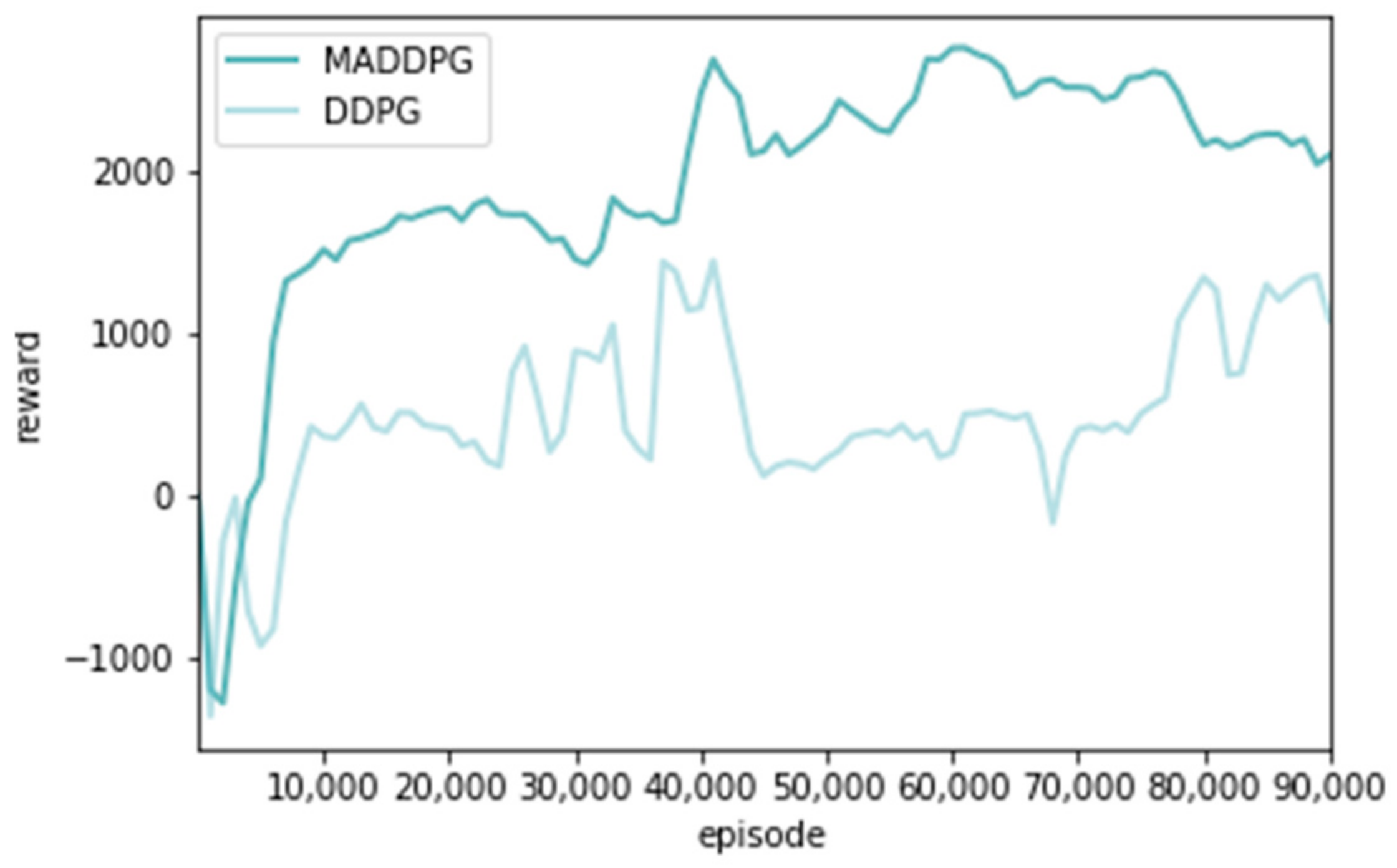
The average cumulative reward distribution in the training process of the MADDPG and DDPG algorithms was analyzed, respectively [29], as shown in Figure 7. The horizontal axis represents the number of pieces of training, and the vertical axis represents the total reward obtained. With an increase in the number of training steps, the reward value of the two algorithms showed a zigzag trend at first and then gradually stabilized. However, the reward value of the DDPG algorithm is always low and has a relatively stable trend after 9000 steps, while the MADDPG algorithm can gradually stabilize after around 7000 steps. So, the MADDPG algorithm has faster convergence than the DDPG algorithm.
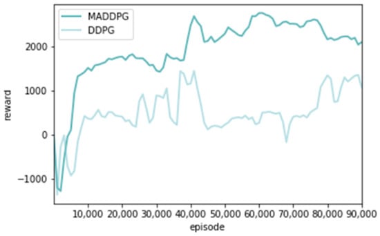
Figure 7.
Different algorithm reward comparison curve.
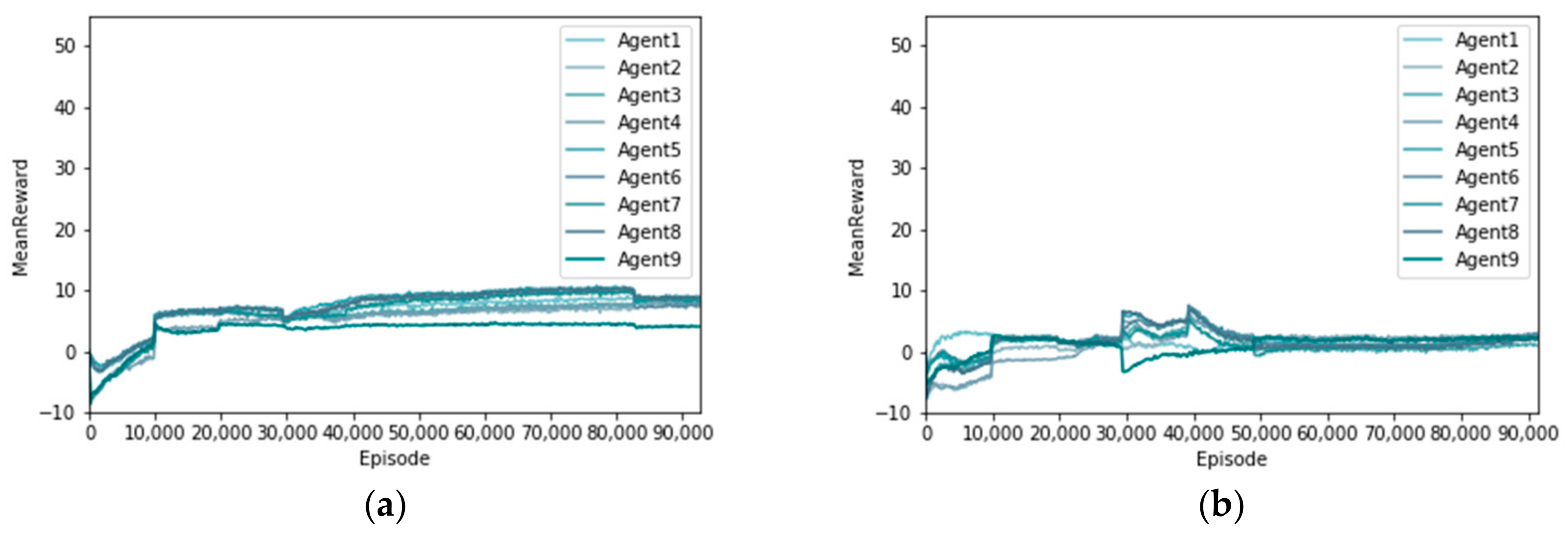
Two reinforcement learning methods were used to solve the scheduling problem of multimetal and multiobjective ore-blending in open-pit mines. The distribution of the rewards obtained by each agent was analyzed. As shown in Figure 8, the horizontal axis represents the number of training sessions, and the vertical axis represents the rewards received by each agent [30]. Figure 8a shows the distribution of rewards using the MADDPG algorithm. From a global perspective, the growth trend of rewards for each agent is similar, with rewards rising first and then gradually flattening. Figure 8b shows the distribution of the rewards using the DDPG algorithm. Globally, there are great differences in the rewards obtained by each agent. By comparing the agent reward distribution of the two algorithms, it can be understood that each agent in the MADDPG algorithm can sense the other agent and co-operate with each other to make efforts toward the goal of reducing the grade and lithology deviation of a polymetallic open-pit mine.
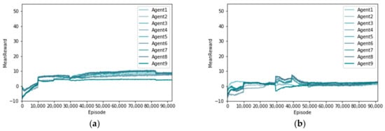
Figure 8.
Rewards for each agent with different algorithms. (a) MADDPG; (b) DDPG.
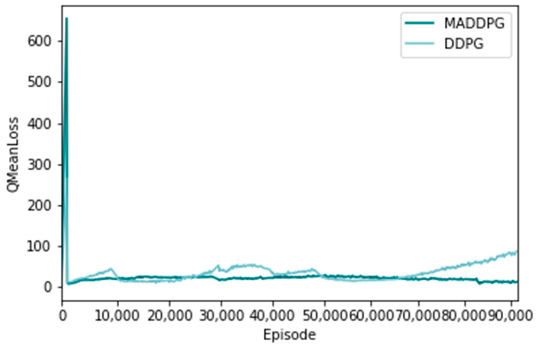
Figure 9 and Figure 10 show the distribution of the loss function of the policy network and the value network using the MADDPG algorithm and the DDPG algorithm, respectively, representing the difference between a single training sample and the real value [31]. The horizontal axis represents the number of training sessions, and the vertical axis represents the average loss of the actor network loss function. From the overall trend, the loss of the MADDPG algorithm shows a zigzag downward trend, which indicates that its network fitting effect is good. The loss function of the DDPG algorithm fluctuates up and down, and the final loss is larger than that of the MADDPG algorithm, indicating that its network fitting effect is not good.
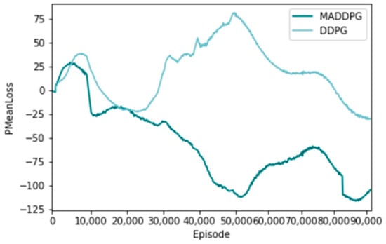
Figure 9.
Loss value of policy network loss function.

Figure 10.
Evaluating the loss value of the network loss function.
5. Conclusions
- (1)
- Aiming at the multimetal and multiobjective ore-blending optimization problem of open-pit mines, we comprehensively considered the influencing factors that have not been considered in the traditional ore-blending model. The ore grade and lithology index are taken as the objective function, and the oxidation rate, ore quantity, grade, and lithology deviation are taken as constraints. The multimetal and multiobjective ore-blending optimization model of open-pit mines was established, which is more in line with the actual production and operation of a mine, effectively improving the comprehensive utilization rate of open-pit mineral resources;
- (2)
- In this study, a deep reinforcement learning algorithm based on actor-critic was used to optimize the multimetal and multiobjective ore-blending process in an open-pit mine. The ore allocation optimization problem was transformed into a partially observable Markov decision process, and the action taken by the agent was scored by the environment in each time granularity. The agent optimizes the strategy according to the score, and the strategy sequence of each agent is sequentially inferred. At the same time, the multimetal multiobjective ore-blending optimization method of open-pit mining based on multiagent deep reinforcement theory can make online decisions and undertake offline training, obtaining the current ore-blending strategy in real-time and this can be fed into production operations;
- (3)
- A simulation experiment method was used to test the ore-blending optimization model, and the ore-blending process was liberated from the traditional static ore-blending method. The changes in ore grade, lithology, oxidation rate, and ore quantity within each time granularity in the ore-blending optimization process can be observed in real-time, which makes the ore-blending process dynamic and helps researchers to clarify the logic behind the ore-blending optimization process. The experimental results show that the algorithm can significantly reduce the waiting time in the case of ensuring calculation accuracy, and this has strong practical value.
Author Contributions
Formal analysis, Q.G.; Data curation, L.W.; Writing—original draft, Z.F. and G.L.; Writing—review & editing, L.C. All authors have read and agreed to the published version of the manuscript.
Funding
This research was funded by the National Natural Science Foundation of China, grant number 52264011; the National Natural Science Foundation of China, grant number 51864046; the China Postdoctoral Science Foundation, grant number 2019M662505.
Data Availability Statement
The data that support the findings of this study are available from the corresponding author upon reasonable request.
Acknowledgments
The authors would like to thank Dianbo Liu (China Molybdenum Co., Ltd. (China)) for his help in origin data collection.
Conflicts of Interest
The authors declare that there is no conflict of interest regarding the publication of this paper.
References
- Ke, L.H.; He, X.Z.; Ye, Y.C.; He, Y.Y. Situations and development trends of ore blending optimization technology. China Min. Mag. 2017, 26, 77–82. [Google Scholar]
- Wu, L.C.; Wang, L.G.; Peng, P.A.; Wang, Z.; Chen, Z.Q. Optimization methods for ore blending in open-pit mine. Min. Metall. Eng. 2012, 32, 8–12. [Google Scholar]
- Chen, P.N.; Zhang, D.J.; Li, Z.G.; Zhang, P.; Zhou, Y.S. Digital optimization model & technical procedure of ore blending of Kun Yang phosphate. J. Wuhan Inst. Technol. 2012, 34, 37–40. [Google Scholar]
- Ke, L.H.; He, Y.Y.; Ye, Y.C.; He, X.Z. Research on ore blending scheme of Wulongquan mine of Wugang. Min. Metall. Eng. 2016, 36, 22–25. [Google Scholar]
- Wang, L.G.; Song, H.Q.; Bi, L.; Chen, X. Optimization of open pit multielement ore blending based on goal programming. J. Northeast. Univ. 2017, 38, 1031–1036. [Google Scholar]
- Li, G.Q.; Li, B.; Hu, N.L.; Hou, J.; Xiu, G.L. Optimization model of mining operation scheduling for underground metal mines. Chin. J. Eng. 2017, 39, 342–348. [Google Scholar]
- Yao, X.L.; Hu, N.L.; Zhou, L.H.; Li, Y. Ore blending of underground mines based on an immune clone selection optimization algorithm. Chin. J. Eng. 2011, 33, 526–531. [Google Scholar]
- Li, Z.G.; Cui, Z.Q. Multi-objective optimization of mine ore blending based on genetic algorithm. J. Guangxi Univ. Nat. Sci. Ed. 2013, 38, 1230–1238. [Google Scholar]
- Li, N.; Ye, H.W.; Wu, H.; Wang, L.G.; Lei, T.; Wang, Q.Z. Ore blending for mine production based on hybrid particle swarm optimization algorithm. Min. Metall. Eng. 2017, 37, 126–130. [Google Scholar]
- Gu, Q.H.; Zhang, W.; Cheng, P.; Zhang, Y.H. Optimization model of ore blending of limestone open-pit mine based on fuzzy multi-objective. Min. Res. Dev. 2021, 41, 181–187. [Google Scholar]
- Huang, L.Q.; He, B.Q.; Wu, Y.C.; Shen, H.M.; Lan, X.P.; Shang, X.Y.; Li, S.; Lin, W.X. Optimization research on the polymetallic multi-objective ore blending for unbalanced grade in Shizhuyuan mine. Min. Res. Dev. 2021, 41, 193–198. [Google Scholar]
- Feng, Q.; Li, Q.; Wang, Y.Z.; Quan, W. Application of constrained multi-objective particle swarm optimization to sinter proportioning optimizatio. Control Theory Appl. 2022, 39, 923–932. [Google Scholar]
- Rummery, G.A.; Niranjan, M. On-Line Q-Learning Using Connectionist Systems; University of Cambridge, Department of Engineering: Cambridge, UK, 1994. [Google Scholar]
- Watkins, C.; Dayan, P. Q-learning. Mach. Learn. 1992, 8, 279–292. [Google Scholar] [CrossRef]
- Mnih, V.; Kavukcuoglu, K.; Silver, D. Human-level control through deep reinforcement learning. Nature 2015, 518, 529–533. [Google Scholar] [CrossRef] [PubMed]
- Pan, F.; Bao, H. Research progress of automatic driving control technology based on reinforcement learning. J. Image Graph. 2021, 26, 28–35. [Google Scholar]
- Xu, J.; Zhu, Y.K.; Xing, C.X. Research on financial trading algorithm based on deep reinforcement learning. Comput. Eng. Appl. 2022, 58, 276–285. [Google Scholar]
- Shen, Y.; Han, J.P.; Li, L.X.; Wang, F.Y. AI in game intelligence—from multi-role game to parallel game. Chin. J. Intell. Sci. Technol. 2020, 2, 205–213. [Google Scholar]
- Qu, Z.X.; Fang, H.N.; Xiao, H.C.; Zhang, J.P.; Yuan, Y.; Zhang, C. An on-orbit object detection method based on deep learning for optical remote sensing image. Aerosp. Control Appl. 2022, 48, 105–115. [Google Scholar]
- Ma, P.C. Research on speech recognition based on deep learning. China Comput. Commun. 2021, 33, 178–180. [Google Scholar]
- Zhang, K.; Feng, X.H.; Guo, Y.R.; Su, Y.K.; Zhao, K.; Zhao, Z.B.; Ma, Z.Y.; Ding, Q.L. Overview of deep convolutional neural networks for image classification. J. Image Graph. 2021, 26, 2305–2325. [Google Scholar]
- Deng, Z.L.; Zhang, Q.W.; Cao, H.; Gu, Z.Y. A scheduling optimization method based on depth intensive study. J. Northwestern Polytech. Univ. 2017, 35, 1047–1053. [Google Scholar]
- He, F.K.; Zhou, W.T.; Zhao, D.X. Optimized deep deterministic policy gradient algorithm. Comput. Eng. Appl. 2019, 55, 151–156. [Google Scholar]
- Liao, X.M.; Yan, S.H.; Shi, J.; Tan, Z.Y.; Zhao, Z.L.; Li, Z. Deep reinforcement learning based resource allocation algorithm in cellular networks. J. Commun. 2019, 40, 11–18. [Google Scholar]
- Liu, G.N.; Qu, J.M.; Li, X.L.; Wu, J.J. Dynamic ambulance redeployment based on deep reinforcement learning. J. Manag. Sci. China 2020, 23, 39–53. [Google Scholar] [CrossRef]
- Kui, H.B.; He, S.C. Multi-objective optimal control strategy for plug-in diesel electric hybrid vehicles based on deep reinforcement learning. J. Chongqing Jiaotong Univ. Nat. Sci. 2021, 40, 44–52. [Google Scholar]
- Hu, D.R.; Peng, Y.G.; Wei, W.; Xiao, T.T.; Cai, T.T.; Xi, W. Multi-timescale deep reinforcement learning for reactive power optimization of distribution network. In Proceedings of the 7th World Congress on Civil, Structural, and Environmental Engineering (CSEE’22), Virtual, 10–12 April 2022; Volume 42, pp. 5034–5045. [Google Scholar]
- Lowe, R.; Wu, Y.; Tamar, A. Multi-agent actor-critic for mixed cooperative-competitive environments. In Proceedings of the 31st International Conference on Neural Information Processing System, Long Beach, CA, USA, 4–9 December 2017; pp. 6382–6393. [Google Scholar]
- Li, J.N.; Yuan, L.; Chai, T.Y.; Lewis, F.L. Consensus of nonlinear multiagent systems with uncertainties using reinforcement learning based sliding mode control. IEEE Trans. Circuits Syst. I Regul. Pap. 2023, 70, 424–434. [Google Scholar] [CrossRef]
- Dao, P.N.; Liu, Y.C. Adaptive reinforcement learning in control design for cooperating manipulator systems. Asian J. Control 2022, 24, 1088–1103. [Google Scholar] [CrossRef]
- Vu, V.T.; Pham, T.L.; Dao, P.N. Disturbance observer-based adaptive reinforcement learning for perturbed uncertain surface vessels. ISA Trans. 2022, 130, 277–292. [Google Scholar] [CrossRef]


Disclaimer/Publisher’s Note: The statements, opinions and data contained in all publications are solely those of the individual author(s) and contributor(s) and not of MDPI and/or the editor(s). MDPI and/or the editor(s) disclaim responsibility for any injury to people or property resulting from any ideas, methods, instructions or products referred to in the content. |
© 2023 by the authors. Licensee MDPI, Basel, Switzerland. This article is an open access article distributed under the terms and conditions of the Creative Commons Attribution (CC BY) license (https://creativecommons.org/licenses/by/4.0/).