Abstract
The choice of attributes in the multi-attribute decision-making process becomes frequently uncertain because of the diverse degree of preference for alternatives. These are assessed utilizing human decisions and linguistic terms that can be utilized for a more adaptable and delicate assessment. The present article illustrates a multi-attribute decision-making (MADM) process, named the exponential technique for order of preference by similarity to an ideal solution (Exp-TOPSIS), considering the selection of attributes with existing uncertainty. Another three notable multi-attribute decision-making (MADM) processes, termed as multi-attribute utility theory (MAUT), elimination and choice expressing reality method (ELECTRE), and the technique for order of preference by similarity to an ideal solution (TOPSIS) are utilized to present a comparison with the proposed methodology by proposing a mathematical model for a solid transportation problem intending to minimize carbon emissions under an uncertain environment. The uncertainty theory, which depends on human conviction degree, is utilized to define the uncertain parameters of the model related to the problem. Applying the proposed one and the other three multi-attribute decision-making processes, the best emission factors are observed to mitigate the carbon emissions from the transport sectors. In this context, the proposed method has some advantages over the existing techniques in selecting the emission factors. All four MADM approaches with different weights have been tested to choose the best five attributes among nine options to be utilized in the mathematical model to minimize the total carbon emission ejection from transportation. In every case, the obtained result states that the proposed Exp-TOPSIS gives the minimum carbon emissions in a range of 2100–2500 units. LINGO 13.0 solver is used to address the deterministic solid transportation problem, and finally, this study presents some investigations on the selection of carbon emission factors and future utilization of the proposed multi-attribute decision-making process.
1. Introduction
Many factors are responsible for global warming, and carbon emissions are the most significant. Carbon emissions also assume an essential part in expanding the ozone-depleting substances. Carbon emissions are brought about by industry, transportation, private areas, businesses, horticultural areas, and so forth. The transportation sector is one of the world’s most elevated carbon emission sectors and was responsible for roughly 61% of worldwide oil utilization, 28% of energy utilization, and 22% of carbon emissions in 2012 [1]. Thus, a decrease in carbon emissions from the transportation area is difficult in the present reality. In street transport, carbon emissions essentially rely upon fuel type, vehicle type, street conditions, climate conditions, traffic conditions, ringing framework, load conditions, vehicle productivity, driver effectiveness, and so on. Along these lines, the greater part of the carbon emission decrease drives has focused on supplanting energy-inept equipment and facilities, upgrading items and bundling, finding less dirtying energy sources, executing energy-saving systems [2], etc. Renewable power sources such as sun-based energy and biodiesel are less destructive to the climate. Yet, it is hard to recognize which kind of energy is more destructive as the case is completely unsure. Since, in the case of choosing a vehicle, if the decision is made between a truck, tripper, and pick-up van, a pick-up van may discharge less carbon; however, a truck can convey more load [3]. Thus, experts will be confounded to choose the less harmful vehicle. If there should arise a question of the street conditions, additionally, this vulnerability is pertinent too. A plain street will cause less outflow than a bumpy street. In any case, if the bumpy street is more limited then experts might pick a sloping street to decrease the expense. Driver effectiveness is another criterion that incurs a cost as well. The driver who has huge experience will demand more compensation than the less experienced driver. Be that as it may, the driver with huge experience will transmit less carbon as he has great driving expertise. If the decision-makers think about cost, then a less experienced driver will be chosen, otherwise not. Therefore, sometimes, the decision-making process may be influenced by the cost of carbon emissions, leading to an uncertain decision-making process.
An uncertain environment is utilized to manage such a sort of vulnerability. There are various sorts of uncertain variables, viz., fuzzy variables such as triangular, trapezoidal, normal, gamma, fuzzy rough variables, stochastic fuzzy variables, uncertain variables [4] such as linear, zigzag, normal, log-normal, and so on. In the literature, such methodologies have been created by a significant proportion of scientists to deal with these dubious cases; however, this study uses the uncertainty theory developed by Liu [4] in 2007 and it is a part of mathematics that relies on normality, duality, subadditivity, and product axioms. The significant contribution to uncertainty theory by Liu et al. [5], gives a wide applicability of uncertain theory to many real-life cases. The expected value function of uncertainty theory is presented in [6]. The uncertain multi-objective and goal programming is shown in [7]. Like Liu, there are several authors who have proposed different models considering uncertainties. Cui and Sheng presented a solid transportation problem (STP) for multi-item in [8]. In their multi-objective models, several uncertain parameters were considered to depict the real-life scenario. Sheng and Yao studied a transportation model based on uncertainty theory [9]. Stochastic scheduling of aggregators of plug-in electric vehicles for participation in energy and ancillary service markets in an uncertain environment is shown in [10].
Decision-makers always find it difficult to take the optimum decision while dealing with uncertainty. Therefore, over the years, uncertainty theory has been significantly studied and applied in many areas to make the decision more realistic. Moreover, the decision-making process involves alternatives and multiple criteria to obtain the best decision. In some multi-criteria decision-making (MCDM) processes, alternative methods for the determination of group decision-making have been improved by Rosanty et al. [11]. This method was created to decide the best option from several alternatives, dependent on the criteria in making decisions. One of the techniques in the decision-making group is MCDM. MCDM is separated into two models: multi-attribute decision-making (MADM) and multi-objective decision-making (MODM). In our study, this MADM approach has been conducted with the utilization of zigzag uncertain factors to show the distinctive characteristics of carbon emissions. The ranking is also shown for how to choose the best and worst criteria for carbon emission selection. To introduce those things, four sorts of MADM approaches have been introduced such as multi-attribute utility theory (MAUT), elimination and choice expressing reality method (ELECTRE), the technique for order of preference by similarity to an ideal solution (TOPSIS), and the proposed exponential technique for order of preference by similarity to an ideal solution (Exp-TOPSIS). Exp-TOPSIS is only the augmentation of the TOPSIS method with an exponential function which was not studied earlier by any researchers, according to our literature survey. In the case of Exp-TOPSIS, the normalized matrix is taken as an exponential function which will be illustrated later.
1.1. Research Motivation
This study deals with carbon emissions and their calculation through different MADM processes. In today’s world, carbon emissions cause very serious ecological problems. By seeing this situation in the real world, we have assumed to draw a carbon emission solid transportation model and defined MADM methods to show the alternatives that are responsible for carbon emissions.
1.2. Research Objectives
The main objectives of this study are as follows:
- Different types of MADM approaches, viz., MAUT, ELECTRE, TOPSIS, and Exp-TOPSIS have been stated, step by step.
- Exp-TOPSIS has been proposed which is the expansion of the TOPSIS method.
- A case study of carbon emissions is shown with the use of some practical data in the form of zigzag uncertain variables.
- An STP has been proposed to show the application of MADM methods.
- All the MADM methods have been utilized to present the ranking with different weights of attributes and also with the same weights of attributes.
- From those rankings, the best five have been taken, and accordingly, these are used to solve the proposed STP with the use of Lingo 13.0 iterative software.
The main scope of this study is that it will help the researchers to find optimal carbon emissions by selecting different types of alternatives to the MADM process.
The organization of the article is as follows. Section 2 presents the literature review. Basic concepts of the uncertain theory are discussed in Section 3. The steps involved in decision-making processes are shown in Section 4. In Section 5, a case study with some practical data are shown. With the use of the case study, a mathematical model for an STP is also proposed. In Section 6, a solution using MADM is described. Results and analysis are shown in Section 7. In Section 8, the conclusion and future aspects have been presented.
2. Review of the Relevant Literature
Multiple studies in the literature have applied MADM/MCDM approaches to analyze decision-making under uncertainty for carbon emissions [12]. MADM/MCDM is a method to select the most convenient solution among the available criteria chosen by a decision-maker [13,14]. Zopunidis et al. [15] described the multi-criteria decision-aid classification methods. Anand et al. [16], in 2008, described the application of MCDM in a robotic system using a fuzzy analytical hierarchy process. Fuzzy multi-criteria decision-making has been described by Carlsson et al. [17]. Kundu et al. [18] proposed a fuzzy multi-criteria decision-making approach to finding the most preferred transportation mode among available modes with respect to some evaluation criteria for a solid transportation problem (STP). On the other hand, Samanta et al. [19] proposed a model that can cope with the ambiguity and vagueness of an STP. In the first stage of their proposed method, the transportation mode is selected and in the second stage, they solve a multi-product transportation problem.
A multi-attribute decision-making process was presented by Ribeiro et al. [20], in 1996. Different researchers [10,21,22] described the fuzzy multi-criteria decision-making process to select from different attributes. Guzel et al. [23] dealt with a multi-attribute solid transportation system where supply and demand are considered uncertain, and they applied a goal programming approach to deal with multiple objectives. Roy et al. [24] addressed the complexity of fixed-charged solid transportation problems and proposed a new ranking method. Roy [25] discussed the multi-criteria methodology for decision-aiding, in 1996, and also discussed the ELECTRE methods in [26]. A brief discussion of ELECTRE and TOPSIS has been shown in [26,27], respectively. MCDM/MADM has different categories of approaches such as a unique synthesis criterion approach, outranking synthesis approach, and iterative total judgment approach. MAUT, ELECTRE, and TOPSIS have been utilized in this study along with a proposed method named Exp-TOPSIS.
A great concern for today’s world is carbon emissions. Therefore, researchers around the world are trying to make a contribution by proposing various models to reduce carbon emissions, and an STP for carbon emissions is one of them. The STP is a generalization of traditional transportation problems (TP) invented by Haley [28]. In the TP, the capacity and demand are considered constraints whereas, in the STP, the mode of the vehicle is an added constraint along with the capacity and demand. Das et al. [29] discussed an STP with mixed types of constraints in different environments. Kundu et al. [30] discussed a multi-objective multi-item STP in a fuzzy environment. Halder et al. [31], Sinha et al. [32], and Das et al. [33] all discussed an STP considering different real-life scenarios and proposed the related mathematical models in different environments such as fuzzy, type-2 fuzzy, and rough intervals, respectively. Researchers have made different types of mathematical models for an STP considering carbon emissions. Salehi et al. [34] described green transport planning with speed control: a balance between total transport costs and carbon emissions. Das et al. [34] discussed a green STP and successfully proposed and solved a model related to a green STP with the use of type-2 fuzzy variables.
A linear programming model is proposed by Soysal et al. [35] in an effort to make the logistics network sustainable by minimizing greenhouse emission gas and cost. Another effort to reduce carbon emissions in the supply chain networks is given by Pan et al. [36]. Chiu et al. [37] described the equivalence of energy prices for carbon taxes and emission trading. In today’s world, the selection of factors that caused carbon emissions with the help of MCDM and MADM methods has become an interesting and integral part of the dynamic research of sustainable supply chain management [38]. Tzeng et al. [39] discussed a multi-criteria analysis of alternative-fuel buses for public transportation energy policy. Wang et al. [27] presented the TOPSIS for fuzzy multiple criteria group decision-making. Watkiss et al. [37] discussed the social cost of carbon review. A multi-class multi-criteria network equilibrium was presented by Yang et al. [38], in 2004. Yeh et al. [40] discussed a modeling subjective evaluation for a fuzzy group MCDM. For more knowledge about multi-attribute decision-making, readers can refer to the “multiple attribute decision-making: methods and applications” by Hwang et al. [41].
The presented literature reviews clearly state the art of this research; as a shred of evidence, it is observed that no such study exists that reflects the art of proposing an Exp-TOPSIS to a sustainable supply chain management problem, i.e., to solve a model of STP that minimizes the carbon emission factors considering uncertainty. Additionally, this article would be of great interest to its readers due to the following major contributing discussion in a very simple and familiar manner:
- In this paper, taking uncertainty into account, four different MADM techniques have been discussed and MAUT is one of them. As the preferences are used as the input in this technique, these preferences should be precise [42,43]. This study incorporates this method to solve a sustainable STP model since it can be applied to many fields, namely, agriculture, energy management, finance, and others. Section 4.1 presents detailed explanations of this process.
- The ELECTRE is one of the techniques which can be applied, which takes uncertainty and vagueness into account, and is presented in [44]. The process and its results can be difficult to explain simply; upping the rankings means that the strengths and weaknesses of the alternatives are not directly identified. This study uses this method in the solution process of the proposed mathematical model, and the related detailed explanations are available in Section 4.2.
- Because of the simple methodological aspect of the TOPSIS, this study considers this method as well [45,46]. The correlation of attributes sometimes makes it difficult to keep the consistency of judgment in many MCDM methods, whereas TOPSIS does not focus on the correlation between attributes. It has applications in many areas such as logistics and supply chain management, engineering, production systems, sales and marketing, environment, human resource management, and water resources. The detailed utilization of TOPSIS in solving the proposed model is available in Section 4.3.
- Finally, the Exp-TOPSIS, a modified version of the TOPSIS, was developed with a change in the technique of giving preferences to orders by similarity to ideal solutions based on the exponential function. As the exponential function indicates the rate of change in expression to the most recent one, it is giving them more realistic and accurate multi-criteria-based decisions. Thus, it is proposed and used hereby in this research article to solve a real-life-based case study designated to a supply chain-oriented optimization problem. Section 4.4 gives detailed explanations of this method.
As an application to the proposed method, a case study is presented and the place for the study is the chosen state “Tripura” of India, which is a hilly area connected by roadways mainly to India, resulting in a huge amount of carbon emissions from transportation to this state.
3. Basic Concepts of Uncertainty Theory
In this study, the main focus is to concentrate on the MADM approaches with the assistance of uncertain variables. A concise depiction of all the fundamental concepts has been given below.
From a mathematical point of view, uncertainty theory is essentially an alternative to estimation. Uncertainty theory should start with a measurable space and rely on several sets such as algebra, σ-algebra, measurable set, Borel-algebra, Borel sets, and measurable functions. Some definitions of uncertainty theory need to be discussed. To provide an axiom-based mathematical tool for describing and dealing with inaccuracies in practice, Liu [45] introduced the uncertainty theory and also successfully applied it to manage and solve optimization problems. To complete this study, some basic concepts and definitions of uncertainty theory have been introduced below.
3.1. Definition
Let us consider a non-empty set Г and a σ-algebra L over Г. Then, for every measurable set Ʌ, the triplet (Г; L; M) will be termed as an uncertainty space for the uncertain measure M subject to fulfilling the axioms given below.
Axioms 1: M {Г} = 1, which can be termed as the normality axiom.
Axioms 2: M {Ʌ} +M {Ʌc} = 1 for any event Ʌ ∈ L, which can be termed as the duality axiom.
Axioms 3: For every countable sequence of events Ʌ1, Ʌ2, …, it can be expressed as
and it can be termed as the subadditivity axiom. Note that the triplet (Г; L; M) is defined as the uncertainty space.
3.2. Theorem
According to Yang et al. [46], “A monotone increasing function defined as ξ: ℜ→ [0, 1] will be called an uncertainty distribution if and only if the function’s monotonicity is continuous excluding Θ(x) ≡ 0 and Θ(x) ≡ 1”.
The use of uncertain variables in real-life decision-making problems is very often. There are mainly four different types of uncertain variables that can be observed and defined based on different membership patterns (Gaussian or normal, zigzag, linear, and log-normal) for the data set. This study is developed by considering the zigzag uncertain variable as the parameter for the proposed model. A brief description of zigzag uncertain variables is given below.
A variable that is uncertain denoted by , with the condition for , is called zigzag if it is following a zigzag uncertainty distribution:
Figure 1 shows the zigzag uncertainty distribution, where are the zigzag uncertain variables and Θ(x) represents the distribution of the zigzag uncertain variables.
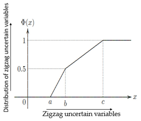
Figure 1.
Zigzag uncertainty distribution.
To simplify the use of the zigzag uncertain variable, it has to be converted to equivalent crisp form using the reduction method based on the expected value. In the paper of Yang et al. [46], the method of reduction based on the expected value is shown below:
4. Decision-Making Process
This research is mainly based on the MADM process and in this context, this article intends to present four types of MADM approaches, viz., MAUT, ELECTRE, TOPSIS, and the proposed Exp-TOPSIS. Hence, it is required to explain all these four methods in a detailed manner so that the use of them can be easily catchable and thus, all the steps to these four processes are described as follows.
4.1. Multi-Attribute Utility Theory
MAUT [43] depends on different attributes which have been chosen by the decision-makers. Sometimes, in MAUT, “objectives” are used in the case of “attributes”. The multi-attribute value theory (MAVT) is also used in attribute selection. The difference between MAUT and MAVT is that the utility function does not include the decision-maker’s risk appetite, whereas the value function does. The utility function is also a value function, but the value function does not necessarily have to be a utility function. Considering a set of different alternatives denoted by and a set of criteria for decision-making denoted by , the problem can be articulated in such a way that defines the execution of the alternative with respect to the criterion .
The steps of MAUT can be described as below:
Step 1. The multi-attribute utility function assumes that there are criteria, and for each of those criteria, a one-dimensional utility (or value) function is evaluated or can be evaluated.
Step 2. The overall utility for the alternatives is expressed by aggregating all the utility functions. Moreover, the process of aggregation is based on the weighting of several criteria and these criteria are considered in the utility function according to their importance. The relationship between the weights of different criteria represents a trade-off of the criteria. The most commonly used multi-attribute utility function is the linear additive utility function:
where is defined as the sum of and and represents the total utility measure of the alternative or the priority of the alternative . Here, is representing the priority weight for the criterion . The above expression for assumes that the execution value is already in the utility scale. Usually, this is mandatory,
otherwise, the increase in the weights will directly increase the utility, always. The trade-offs between the criteria and can be calculated from the ratio of the weights .
Step 3. Normally, the calculation of the marginal rate that helps in the substitution between the two criteria and is performed as the ratio of partial derivatives associated with the utility functions and is given below:
This means that the decision-maker is ready to abandon the λ units of the criteria in order to increase the value of the criteria by one.
4.2. ELECTRE Method
ELECTRE [26] belongs to the outranking method. The ELECTRE method has the following steps which are described below:
Step 1. Creating a decision matrix.
In the decision matrix, columns can indicate the criteria () and rows can indicate the alternatives (). This matrix can be termed the standard matrix and it establishes the base for the process.
Step 2. Normalization of the decision matrix.
The process of normalization of the decision matrix obtained in step 1 consists of the following formula:
Using the formula given in Equation (2), one can obtain the following normalized decision matrix denoted as .
Step 3. Weight preference for the normalized decision matrix.
The decision-maker can choose the weight in such a way that their sum will result in 1. The weight can be multiplied with the corresponding normalized decision matrix terms, such as
where is the weighted normalized decision matrix. One can observe the diagonal property of the matrix , as all the entries are diagonal as , and the rest of the other entries are zero.
Step 4. Concordance and discordance set creating.
The data obtained in the final weighted normalized matrix are then taken into consideration for the comparison pairwise and the results are obtained as follows.
If in each pair, each alternative is superior compared to the other pair element, then it can be granted as a set member of the concordance set, which can be denoted as and defined as follows,
or, in the other case, i.e., when the alternative is inferior compared to the other pair element, then that particular element of the pair for the relevant criteria is granted in the discordance set, which can be denoted as and defined as follows:
Step 5. Creating the concordance matrix.
A concordance matrix is a matrix created by summing up the weight values of the elements of a concordance set. The formula is given below.
Step 6. Creating the discordance matrix.
The discordance matrix is created by dividing the scores of the members of the discordance set by the total score of the entire set.
Step 7. Formulation of the advantage calculation.
The score of the concordance and discordance are averaged. In a concordance matrix, any value above the mean (including ) can be reported as Yes. In the discordance matrix, any value less than or equal to the mean can be specified as no.
Step 8. Creating the net discordance and concordance matrix.
Net discordance and concordance scores can be obtained and utilized to rank the alternatives. Then, the final rank can be computed using the formula given below:
4.3. TOPSIS Method
In 1981, Hwang and Yoon [44] proposed the TOPSIS method, and this method is based on the concept that the superior alternative is the one closest to the positive ideal solution and farthest from the negative ideal solution.
The first three steps (step 1, step 2, and step 3) of TOPSIS are the same as ELECTRE, i.e., first, there is the need to create a decision matrix, then the decision matrix needs to be normalized, and after that, the weight preference for the normalized decision matrix needs to be calculated. Readers can refer to Section 4.2 for a detailed explanation.
Step 4. Using the formulas given below, one can find the positive and negative ideal solutions, respectively:
where and are linked with the positive and negative criteria, respectively.
Step 5. Next, the -dimensional Euclidean distance is applied to compute the separation measures. The separation between every alternative and the positive ideal solution is given below:
Similarly, the separation between every alternative and the negative ideal solution is given below:
Step 6. The relative closeness degree to the ideal solution requires computing and it is defined for the alternative with respect to as follows:
Step 7. Sort your preferences in ascending order. A high value of the closeness coefficient suggests that the alternative is performing well. The optimal alternative is the one that comes closest to the ideal solution in terms of relative closeness.
4.4. Proposed Exp-TOPSIS
Exp-TOPSIS is nothing but an extension of the TOPSIS method. In the case of the Exp-TOPSIS, each value of the normalized decision matrix has been taken as the exponential function of the original decision matrix terms. The steps involved in it are described below.
Step 1. The first step of the method is the same as the step given in Section 4.2.
Step 2. Normalization of the decision matrix.
The process of normalization of the decision matrix obtained in step 1 consists of the following formula:
Using the formula given in Equation (14), one can obtain the following normalized decision matrix, denoted as :
Step 3. Weight preference for the normalized decision matrix.
Weight obtained by a decision-maker’s choice can be multiplied with each value of the normalized decision matrix as shown in Equation (3), where is the weighted normalized matrix, is the weight, and is the member of the normalized decision matrix. One can observe the diagonal property of the matrix , as all the entries are diagonal, as , and the rest of the other entries are zero.
Step 4. Compute the positive and negative ideal solutions using Equations (9) and (10), respectively, which is the same as the TOPSIS method.
Step 5. Using the -dimensional Euclidean distance to compute the separation measures. and to calculate the separation of every alternative from the ideal solution, Equations (11) and (12) are to be used.
Step 6. The relative closeness degree to the ideal solution requires computing and it is defined for the alternative with respect to in Equation (13).
Step 7. Sort your preferences in ascending order. A high value of the closeness coefficient suggests that the alternative is performing well. The optimal alternative is the one that comes closest to the ideal solution in terms of relative closeness.
5. Case Study: A Carbon Emission Solid Transportation Problem
A case study has been offered in this section to demonstrate the implementation of the proposed MADM techniques in an uncertain environment. To maximize carbon emissions from vehicles utilized in the transportation sector, a constraint-based mathematical problem with one objective function has been devised. In an uncertain environment, the MADM technique was used to select the optimum parameters for reducing carbon emissions.
5.1. Case Study Related to Carbon Emissions
Tripura is a hilly state situated in northeast India. In Tripura, trucks, trippers, minivans, dumpers, pick-up vans, etc., are the commonly used freight transportation modes. Tripura is bordered by Bangladesh on three sides. Only on one side is India’s mainland connected with Tripura. The map of Tripura is shown in Figure 2.
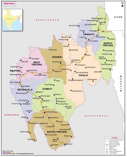
Figure 2.
Physical map of Tripura (https://www.mapsofindia.com/, accessed on 19 March 2023).
Nowadays, the number of vehicles is growing rapidly. Therefore, it is a great concern for the environment in the small state of Tripura. Agartala is the capital of Tripura and Udaipur is one of the biggest cities in Tripura. A study within these two cities has been focused on. In the case of environmental pollution, carbon emissions caused by road transport vehicles are a great matter of concern. Carbon emissions depend on different factors such as fuel type, vehicle type, road conditions, weather conditions, traffic conditions, tolling system, load conditions, vehicle efficiency, driver efficiency, etc.
5.2. Case Study Related to Solid Transportation Problem
Some data from the “M/S Swasti smoke emission testing center” situated in Udaipur, Tripura and from “Tripura State Pollution Control Board” have been collected. The collected data are then utilized to define the fluctuating unit emission as zigzag uncertain variables according to experts’/experienced businessmen’s opinions. For simplicity, two source points, three demand points, and five conveyances have been taken. The data of emissions have been taken concerning nine different factors. The names of the factors are fuel type, vehicle type, road conditions, weather conditions, traffic conditions, tolling system, load conditions, vehicle efficiency, and driver efficiency. A single objective STP model using emission factors has been proposed and it has been presented in Equation (16) later. In Section 7, the inputs which have been collected from the case study are shown in Table 1. With the use of those inputs, four types of MADM techniques are functional to obtain the best five alternatives which are less harmful to the environment.

Table 1.
Per unit normal emissions for the alternatives.
5.3. Materials and Methods
With the use of the collected data, the analysis and use of the research are shown in this section. To define the mathematical model related to the problem, the following assumptions and terms have been used.
Assumptions:
- The parameters of the problem are defined using the analysis made on the past data and experienced experts’ opinions.
- The transportation problem has involved the transportation of goods from their source point to the demand point using different vehicles and it is an unbalanced problem.
- The problem is focused to make an analysis to choose the best factors that optimize the total carbon emissions from the vehicles.
Sets and indices:
| i | Indices to the distribution center. |
| j | Indices to the demand point. |
| k | Indices to the vehicle type used. |
| l | Indices to the different carbon emission factors. |
| l1 | Set of emission factors proportional to the distance traveled by the vehicle. |
| l2 | Set of emission factors proportional to the load or fuel type used in the vehicle. |
Notations:
| Uncertain emission rate for the vehicle k on the route (i, j) considering the l-th factor. | |
| Uncertain extra per unit carbon emissions for the k-th vehicle due to the l-th factor. | |
| dij | Distance between the i-th source point and the j-th demand point. |
| Uncertain emissions at the per unit rate due to the vehicle’s load. | |
| Uncertain emissions at the per unit rate due to the vehicle’s fuel type. | |
| Efficiency based on per unit uncertain emissions caused by the l-th factor. | |
| Ok | Driver efficiency, driving the k-th vehicle. |
| Ek | Per unit emissions for the vehicle type used in transportation. |
| Uncertain available amount of transported items at the i-th source point. | |
| Uncertain demand from the j-th demand point. | |
| Define the uncertain capacity of the k-th vehicle. |
Mathematical model:
Subject to
5.4. Model Description
The objective function (16) consists of four different terms. The first indicates the emissions and extra emissions if there are any from the vehicle on the route for the -th emission factor. This term per unit emissions is multiplied by the distance to evaluate the total emissions for a particular vehicle and is a decision variable used to define the extra emissions for the -th vehicle and is defined in (17). Since emissions are directly proportional to the load on a vehicle as well as the fuel used, so the second term defines the total emissions due to the load for the vehicle . Here, is a decision variable and is defined in (17), which is used to express that, at a time, one factor (load or fuel type) will be functionary to compute the emissions. The third term defined the emissions based on the efficiency rate for different factors (e.g., driver efficiency or vehicle efficiency). Here, is the decision variable, as defined in (21), using , which is the efficiency rate for the factor under consideration and decided by the decision-makers and experts. The last term is used to define the emission rate for choosing a vehicle based on its type such as a small vehicle, large vehicle, etc. Furthermore, the constraint (18) is a source constraint for the transportation network which means that the total transported amount should be less than or equal to the quantity available at each source point. Similarly, constraint (19) is the demand constraint from the different destinations, and constraint (20) is used to define the vehicle capacity which should be less than or equal to the transported amount. The last constraint (22) is putting the non-negativity restriction on the transportation system.
6. Numerical Analysis
This section may be divided by subheadings. It should provide a concise and precise description of the experimental results, their interpretation, as well as the experimental conclusions that can be drawn.
The problem presented in Section 5.2 is an uncertain problem as the input of the problem, i.e., the emission factor’s inputs, are estimated as the zigzag uncertain variable. The deterministic equivalent problem needs to be found for solving the problem in this study. For this, Liu’s [5,47] uncertainty theory has been utilized and then the MADM approaches discussed in the earlier section have been applied to find the best five factors to optimize the carbon emissions. Some data in the zigzag uncertain variable have been collected with the help of expert opinion. Using these data, four types of MADM approaches, MAUT, ELECTRE, TOPSIS, and the proposed Exp-TOPSIS, have been presented.
6.1. Input Tables
All the inputs are considered as zigzag uncertain variables in this study. The per unit normal emissions caused by all the nine factors have been given in Table 1.
The inputs for the other parameters such as the uncertain available sources have been considered as = (20; 30; 35) and = (24; 25; 26), the uncertain demands are considered as = (18; 21; 23), = (14; 15; 16), = (16; 17; 18), and the uncertain capacities of the vehicles are considered as = (12; 14; 15), = (10; 11; 12), = (7; 8; 9), = (8; 9; 10), and = (11; 12; 13). The distances between each source point and demand point have been given as , , , , , and , respectively.
6.2. Decision-Making Process Using MADM
The decision matrix with the use of the inputs given in Table 1 is shown below. It is obtained with the equivalent values of the zigzag uncertain variables calculated using the expected value-based reduction method given in Equation (1). Nine alternatives () of emission factors, which cause danger in our real world, have been taken into account. These are the fuel type , vehicle type , road conditions , weather conditions , traffic conditions , tolling system , load conditions , vehicle efficiency , driver efficiency . The data obtained from the real world are presented in the input tables which are the normal emission rate caused by the fuel type () to driver efficiency (). In the next part, those abbreviations, starting from to for different alternatives, have been used. One criterion has been taken here as criteria 1 (), where denotes the normal emissions caused by the -th factor. The decision matrix is applicable for all the four MADM methods, viz., MAUT, ELECTRE, TOPSIS, and the proposed Exp-TOPSIS. Two types of weights have been taken according to the decision-maker’s opinion, viz., alternatives with different weights and the same weights. The decision matrix in reduced form is presented in Table 2. Three rows are shown in Table 2, where row 1 denotes the decision matrix of MAUT, ELECTRE, TOPSIS, and Exp- TOPSIS.
Table 2.
Decision matrix using reduced zigzag uncertain variables.
Row 2 is the normalized matrix for ELECTRE and TOPSIS, which has been calculated by Equation (2), given in Section 4.2. Row 3 is the weighted normalized matrix that has been calculated by Equation (3), given in Section 4.2.
6.2.1. Rank Obtained Using MAUT
The steps of MAUT have been described in Section 4.1. The function that represents the overall utility has been considered as
The weights of these criteria are denoted as a1 and denotes the normal emissions for different factors, starting from l1 to l9. The overall utility obtained by Equation (23) is given in Table 3. The obtained utility can decide the rank between the two types of weights. Table 2 represents the decision matrix and by using it, the overall utility has been calculated.
Table 3.
Overall utilities and rank using MAUT method.
6.2.2. Rank Obtained Using ELETRE Method
The use of the ELECTRE method in the step-by-step process is presented with an example from Section 4.2. The ELECTRE method is shown with the zigzag uncertain variables. The decision matrix, normalized decision matrix, and weighted normalized matrix for the same weight and different weights are given in Table 2. With the use of the table, the concordance and discordance matrix can be obtained by using Equations (6) and (7). The concordance and discordance index are presented in Table 4. The average scores associated with the concordance and discordance are considered in the calculation.
Table 4.
Concordance and discordance index for different weights and same weights.
For any concordance index in the concordance matrix, a value greater than or equal to the average is defined as ‘Yes’. Furthermore, any discordance index in the discordance matrix, a value which is lesser than or equal to the average is defined as ‘No’. With the use of these criteria, the ranking between the nine alternatives with the different weights and the same weights can be obtained. The ranking is given in Table 5.
Table 5.
Comparison of ranking using ELECTRE method.
6.2.3. Rank Obtained with TOPSIS Method
The TOPSIS method has some steps which are described in Section 4.3. The three matrices, i.e., the decision, normalized decision, and weighted normalized decision matrices are given in Table 2 and need to be identified to obtain the ranking in the TOPSIS function. Furthermore, the distances between every alternative and the positive and negative ideal solutions are calculated using the methods given in Equations (9) and (10), respectively. It can be observed from row 3 of Table 2, the positive and negative ideal solutions for the different weights are 0.163 and 0.025 and for the same weights are 0.0946 and 0.0907, respectively. Using the Equations (11) and (12), the distance between the positive and negative ideal solutions has been obtained, which is given in Table 6, where and indicate the distances from the positive and negative ideal solutions, respectively. In Table 6, the relative closeness cl+ with the Equation (13) can also be found. The rank obtained by the different weights and the same weights can easily be compared from Table 6.
Table 6.
Distance evaluation and rank in TOPSIS.
6.2.4. Rank Evaluation Using Proposed Exp-TOPSIS
The Exp-TOPSIS method has been proposed which is a slight extension of the TOPSIS method. In the case of the Exp-TOPSIS, the normalized matrix can be in the exponential function of the original normalized matrix. The decision matrix is the same as shown in Table 2. However, the normalized matrix and the weighted normalized matrix are slightly different. Next, the calculation for the normalized decision matrix has been performed using the formula given in Equation (14) and is presented in Table 7. The weighted matrix, which is given in row 2 of Table 7, can be calculated by the formula given in Equation (3). Furthermore, the distance between every alternative and the positive and negative ideal solutions can be calculated using the formula given in Equations (9) and (10). From Table 7, it can be easily observed that the positive ideal and negative ideal in the case of the different weights are 0.3264 and 0.0696, respectively, and in the case of the same weights, they are 0.3175 and 0.0514, respectively.
Table 7.
Reduced normalized decision matrix in case of Exp-TOPSIS.
In row 1 of Table 8, and mean the distance between every alternative and the positive and negative ideal solutions, respectively. The relative closeness between every alternative and the positive and negative ideal solutions can be obtained using the Equation (13). The relative distances in the case of the different and same weights are shown in row 2 of Table 8. In addition, the same table presents the rank obtained from the different weights and same weights.
Table 8.
Distance evaluation and rank in Exp-TOPSIS.
7. Results and Discussion
The ranking obtained from all the four MADM techniques has been compared, after solving the case study with the MADM technique. The comparison has been illustrated below where the different weights are written as and the same weights are written as . = fuel type, = vehicle type, = road conditions, = weather conditions, = traffic conditions, = tolling system, = load conditions, = vehicle efficiency, = driver efficiency.
From Table 9, a comparison of ranking between the different weights and same weights using four MADM techniques can easily be observed. Furthermore, the best five factors have been chosen to calculate the model given in Equation (16), according to the decision-maker’s choice.
Table 9.
Comparison of ranks between four MADM methods.
From Table 9, the results obtained in the different MADM methods can be compared. Two types of weights are taken for the alternatives of emissions. One is with the same type of weightage, 0.11, and another is with different weights. In the case of MAUT, the best five rankings are the fuel type, driver efficiency, vehicle efficiency, vehicle type, and load conditions, respectively, when they are applied to different weights. Vehicle efficiency, fuel type, driver efficiency, traffic conditions, load conditions, and weather conditions are the best five alternatives in the case of the same weights. All the other methods with the same and different weights are also presented.
The best five factors are chosen from Table 9 concerning their activities in the environment. A graphical analysis is illustrated in Figure 3. The figure presents the comparison of the different weights of the best five factors of MAUT, ELECTRE, TOPSIS, and the proposed Exp-TOPSIS given in Table 1. The input of each of the five factors is taken from Table 1 and those are used to calculate each method of MADM using the objective function given in Equation (16). The total emissions for the same weightage calculated by MAUT are 2443.937, ELECTRE are 3561.462, TOPSIS are 3467.150, and by the proposed Exp-TOPSIS are 2435.063 and for the different weightage, MAUT gives 1340.26, ELECTRE provides 3483.67, TOPSIS gives 4589.05, and Exp-TOPSIS provides 4589.05. These are all presented in Table 10.
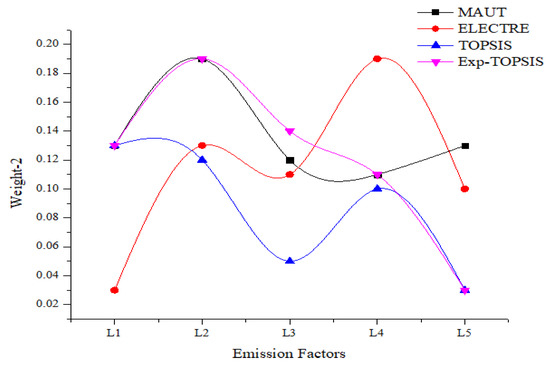
Figure 3.
Best factors calculation for different weights.
Table 10.
Optimal objective value for carbon emissions using different MADM approaches.
7.1. Convergence Test of Proposed Exp-TOPSIS
The MADM approaches with the different weights have been tested. Five types of different weights have been chosen to compare the results. From Table 11, it is clear that the results obtained in the Exp-TOPSIS are better than the other MADM methods in every case.
Table 11.
Optimal result with different MADM techniques.
7.2. Advantage of the Proposed Method
The results presented in Table 10 show an optimal solution with the same weightage and different weightage. The proposed Exp-TOPSIS provides the minimum emissions with the same weightage and with the different weightage, MAUT provides the minimum emissions. In the case of the same weightage, all the weights have been taken as 0.11 which are presented in Table 2. All the alternatives have been multiplied with the same weight to calculate a normalized weighted decision matrix for the same weightage. In Exp-TOPSIS, the best five alternatives are vehicle efficiency, fuel type, vehicle type, traffic conditions, and weather conditions for the same weightage. The objective function of Equation (16) has been calculated and the result has been found as 2435.063 which is less than other methods such as MAUT, ELECTRE, and TOPSIS. Therefore, vehicle efficiency, fuel type, vehicle type, traffic conditions, and weather conditions are five factors that are less harmful to the environment. In the proposed Exp-TOPSIS, the weighted matrix of Table 7, with the use of an exponential function, has been calculated. The exponential function is always the best way to calculate a good and effective result.
In the case of the different weightage, all nine alternatives take nine different weights, given in Table 2. For different weightage cases, MAUT has provided the minimum emissions. In the case of MAUT, the best five factors are the fuel type, driver efficiency, vehicle efficiency, vehicle type, and traffic conditions. When the sum of the weight of those factors from Table 2 has been calculated, it is 0.69. The sum is large as the decision-maker gives more priority to these five factors. Furthermore, in the case of TOPSIS and the proposed Exp-TOPSIS, the sum of the weightage is 0.30 which is less than all four cases. In TOPSIS and the proposed Exp-TOPSIS, the best five factors are the weather conditions, road conditions, driver efficiency, tolling system, and traffic conditions. The results obtained by those alternatives are the largest. Therefore, the proposed method may give a result which is helpful to identify which five alternatives are more harmful to the environment as the total emissions are highest.
7.3. Managerial Insights
The proposed model (Section 5) has been solved using four different MADM processes, including the proposed one also. In each case, the optimal solution has been obtained, with a variation in the optimal objective value which represents the total carbon emissions in the model, and it is required to be minimized. The solution is presented in Table 10, and it has been observed that whenever we consider the same weights for the MADM process, the proposed method, i.e., Exp-TOPSIS, provides us with the optimal objective value for carbon emissions compared to the other three processes. In Figure 4, it is observed that the minimal objective value is 2434.063 and has been obtained for Exp-TOPSIS, which is the proposed one.
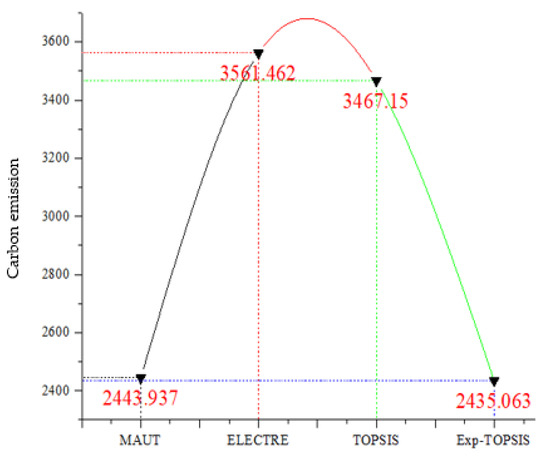
Figure 4.
Optimal carbon emissions obtained with four MADM process taking same weights.
From this result, the following managerial insights have been drawn:
- Same weights mean giving the same preferences to all the attributes, which defines the uniformity and unbiasedness for a fair comparison to the performance of four MADM processes and it is observed that the proposed MADM process gives the best minimal carbon emission. Hence, a decision-maker can choose the proposed method not only to optimize carbon emissions but other optimization problems such as the optimization of cost, time, profit, social economic disruption, etc.
- The Exp-TOPSIS is based on the exponential function, and it always gives the rate of the change in expression that is related to a particular decision-making attribute. Thus, it is suggested to use the proposed method when the case of decision-making is sensitive. The results obtained for the proposed model can be considered as evidence.
- The proposed mathematical model is an optimization model originating from a linear programming problem; thus, it opens several ideas to use in a different situation where the objective is to optimize with respect to the given constraints. For example, traveling means sales problems, job assignment problems, cold supply chain-based inventory problems, vehicle routing problems, facility locations problems, etc., considering uncertainty.
- This study also analyzed the impact of choosing different weights in the objective value and this is observed in Table 10, and also in Figure 5, which represents the same with a comparison to the case if we choose the same weights. Here, for the different weights, ELECTRE gives the optimal emissions, as this process consists of elimination and choice based on the expression of reality, rather than the rate of change in expression. This process is okay sometimes when the expression is available in reality but it is very rare and of high risk; thus, our proposed process would be a better one from a reliability point of view.
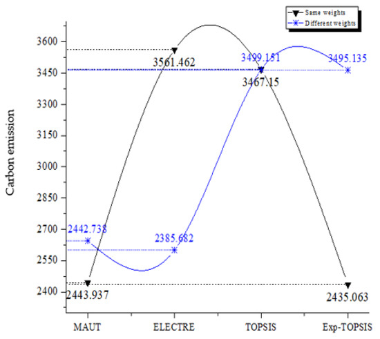 Figure 5. Optimal carbon emissions obtained with four MADM process.
8. Conclusions and Future Scope
This study proposed an MADM approach based on extending the traditional TOPSIS method. Three different types of MADM, viz., MAUT, ELECTRE, and TOPSIS have been illustrated to make a comparison. The main research objective of this study was to minimize carbon emissions using different alternatives and different MADM processes. The main scope of this study is to find the optimum carbon emissions which will benefit the eco-friendly environment. All this study is related to a green solid transportation problem.
Furthermore, a case study has been presented in this paper, and the practical data have been collected and implemented in the solution process of a mathematical model developed for the stated problem. The inherent uncertainty of the practical data set is dealt with using zigzag uncertain variables. Uncertain variables deal with the uncertainty of the environment. We are not able to ensure whether anything happens or not in our natural world. The main merit of uncertain variables is that they help to find a more accurate result when we defuzzify them from more than one value. The demerit is that it is complicated to calculate the formulas using these zigzag uncertain variables. An objective function concerning carbon emissions has been proposed in the mathematical model to minimize the total emissions from the transportation sectors. The last, final contributing discussion of this research article can be summarized as follows:
- Four MADM processes, MAUT, ELECTRE, TOPSIS, and Exp-TOPSIS, are discussed in a step-by-step manner.
- A novel method of Exp-TOPSIS is proposed, which is the extension of the TOPSIS method.
- A case study of carbon emissions is shown with the use of some practical data in the form of the zigzag uncertain variable.
- A mathematical model for an STP is formulated to show the use of MADM methods.
- All the MADM methods are utilized to present the ranking with the different weights of attributes and the same weights of attributes.
- The proposed STP is solved using Lingo 13.0 iterative software from those five best rankings.
- The managerial insights have been drawn to analyze the results at the end.
As a future augmentation, this study can also additionally be utilized for different sorts of multi-criteria/multi-attribute functions. A wide comparison of different MADM methods can be examined considering different study contexts. The proposed objective function can be additionally reached to explore more critical carbon emission functions. These MADM methods can be utilized for handling inventory management as well. Moreover, delicate methods such as a genetic algorithm, particle swarm optimization, and heuristic search algorithm can be applied for wider study and better outcomes. These MADM methods will also be beneficial to reduce carbon emissions by preparing different models not only in the transportation sector but can be applied in inventory management problems comprising production, reverse logistics, forward logistics, etc. The main scope of this study is that it will help the researchers to find optimal carbon emissions by selecting different types of alternatives to the MADM process.
Author Contributions
Conceptualization, A.D., A.A. and D.S.; methodology, A.D. and A.A.; software, D.S. and A.D.; validation, A.A., I.M.H., U.K.B. and A.D.; formal analysis, A.A., I.M.H., U.K.B. and F.A.; investigation, A.A., I.M.H., D.S. and A.D.; resources, A.D. and D.S.; data curation, A.A. and D.S.; writing—original draft preparation, D.S.; writing—review and editing, A.D., A.A., I.M.H. and M.K.N.; visualization, D.S., A.A. and I.M.H.; supervision, A.D., U.K.B. and I.M.H.; project administration, I.M.H.; funding acquisition, A.A. and I.M.H. All authors have read and agreed to the published version of the manuscript.
Funding
This research is supported by the Researchers Supporting Project number (RSPD2023R533), King Saud University, Riyadh, Saudi Arabia.
Institutional Review Board Statement
Not applicable.
Informed Consent Statement
Not applicable.
Data Availability Statement
Data will be provided on request.
Acknowledgments
We would like to thank the editors of the journal as well as the anonymous reviewers for their valuable suggestions that make the paper more robust and more consistent.
Conflicts of Interest
The authors declare no conflict of interest.
References
- IEA. CO2 Emissions from Fuel Combustion Highlights; IEA: Paris, France, 2015; 139p, Available online: https://iea.blob.core.windows.net/assets/eb3b2e8d-28e0-47fd-a8ba-160f7ed42bc3/CO2_Emissions_from_Fuel_Combustion_2019_Highlights.pdf (accessed on 19 March 2023).
- Choudhary, A.; Sarkar, S.; Settur, S.; Tiwari, M. A carbon market sensitive optimization model for integrated forward–reverse logistics. Int. J. Prod. Econ. 2015, 164, 433–444. [Google Scholar] [CrossRef]
- Seo, J.; Park, J.; Oh, Y.; Park, S. Estimation of Total Transport CO2 Emissions Generated by Medium- and Heavy-Duty Vehicles (MHDVs) in a Sector of Korea. Energies 2016, 9, 638. [Google Scholar] [CrossRef]
- Liu, B. Uncertainty Theory; Springer: Berlin/Heidelberg, Germany, 2007; pp. 205–234. [Google Scholar]
- Liu, Y.; Ha, M. Expected Value of Function of Uncertain Variables. J. Uncertain Syst. 2010, 4, 181–186. [Google Scholar]
- Liu, B.; Liu, B. Theory and Practice of Uncertain Programming; Springer: Berlin/Heidelberg, Germany, 2009. [Google Scholar]
- Liu, B.; Chen, X. Uncertain Multiobjective Programming and Uncertain Goal Programming. J. Uncertain. Anal. Appl. 2015, 3, 73. [Google Scholar] [CrossRef]
- Cui, Q.; Sheng, Y. Uncertain programming model for solid transportation problem. Int. Inf. Inst. Inf. 2013, 16, 1207. [Google Scholar]
- Sheng, Y.; Yao, K. A transportation model with uncertain costs and demands. Information 2012, 15, 3179–3185. [Google Scholar]
- Alam, S.T.; Ahmed, S.; Ali, S.M.; Sarker, S.; Kabir, G.; Ul-Islam, A. Challenges to COVID-19 vaccine supply chain: Implications for sustainable development goals. Int. J. Prod. Econ. 2021, 239, 108193. [Google Scholar] [CrossRef]
- Rosanty, E.S.; Dahlan, H.M.; Che Hussin, A.R. Multi-criteria decision making for group decision support system. In Proceedings of the International Conference on Information Retrieval and Knowledge Management, CAMP’12, Kuala Lumpur, Malaysia, 13–15 March 2012; pp. 105–109. [Google Scholar]
- Ilgin, M.A.; Gupta, S.M.; Battaïa, O. Use of MCDM techniques in environmentally conscious manufacturing and product recovery: State of the art. J. Manuf. Syst. 2015, 37, 746–758. [Google Scholar] [CrossRef]
- Abbasbandy, S.; Asady, B. Ranking of fuzzy numbers by sign distance. Inf. Sci. 2006, 176, 2405–2416. [Google Scholar] [CrossRef]
- Abbasbandy, S.; Hajjari, T. A new approach for ranking of trapezoidal fuzzy numbers. Comput. Math. Appl. 2009, 57, 413–419. [Google Scholar] [CrossRef]
- Zopounidis, C.; Doumpos, M. Multi-criteria decision aid in financial decision making: Methodologies and literature review. J. Multi-Criteria Decis. Anal. 2002, 11, 167–186. [Google Scholar] [CrossRef]
- Anand, M.D.; Selvaraj, T.; Kumanan, S.; Johnny, M.A. Application of multicriteria decision making for selection of robotic system using fuzzy analytic hierarchy process. Int. J. Manag. Decis. Mak. 2008, 9, 75. [Google Scholar] [CrossRef]
- Carlsson, C.; Fullér, R. Fuzzy multiple criteria decision making: Recent developments. Fuzzy Sets Syst. 1996, 78, 139–153. [Google Scholar] [CrossRef]
- Kundu, P.; Kar, S.; Maiti, M. A fuzzy MCDM method and an application to solid transportation problem with mode preference. Soft Comput. 2013, 18, 1853–1864. [Google Scholar] [CrossRef]
- Samanta, S.; Jana, D.K. A multi-item transportation problem with mode of transportation preference by MCDM method in interval type-2 fuzzy environment. Neural Comput. Appl. 2019, 31, 605–617. [Google Scholar] [CrossRef]
- Ribeiro, R.A. Fuzzy multiple attribute decision making: A review and new preference elicitation techniques. Fuzzy Sets Syst. 1996, 78, 155–181. [Google Scholar] [CrossRef]
- Triantaphyllou, E.; Chi-Tun, L. Development and evaluation of five fuzzy multiattribute decision-making methods. Int. J. Approx. Reason. 1996, 14, 281–310. [Google Scholar] [CrossRef]
- Abdullah, L. Fuzzy Multi Criteria Decision Making and its Applications: A Brief Review of Category. Procedia Soc. Behav. Sci. 2013, 97, 131–136. [Google Scholar] [CrossRef]
- Güzel, N.; Alp, S.; Geçici, E. Solving solid transportation problems under uncertain environment using goal programming. J. Ind. Eng. 2022, 33, 130–144. [Google Scholar]
- Roy, S.K.; Midya, S. Multi-objective fixed-charge solid transportation problem with product blending under intuitionistic fuzzy environment. Appl. Intell. 2019, 49, 3524–3538. [Google Scholar] [CrossRef]
- French, S.; Roy, B. Multicriteria Methodology for Decision Aiding. J. Oper. Res. Soc. 1997, 48, 1257. [Google Scholar] [CrossRef]
- Roy, B. The Outranking Approach and the Foundations of Electre Methods, Readings in Multiple Criteria Decision Aid; Springer: Berlin/Heidelberg, Germany, 1990; pp. 155–183. [Google Scholar] [CrossRef]
- Wang, Y.-J.; Lee, H.-S. Generalizing TOPSIS for fuzzy multiple-criteria group decision-making. Comput. Math. Appl. 2007, 53, 1762–1772. [Google Scholar] [CrossRef]
- Haley, K.B. New Methods in Mathematical Programming—The Solid Transportation Problem. Oper. Res. 1962, 10, 448–463. [Google Scholar] [CrossRef]
- Das, A.; Bera, U.K.; Das, B. A solid transportation problem with mixed constraint in different environment. J. Appl. Anal. Comput. 2016, 6, 179–195. [Google Scholar] [CrossRef]
- Kundu, P.; Kar, S.; Maiti, M. Multi-objective multi-item solid transportation problem in fuzzy environment. Appl. Math. Model. 2013, 37, 2028–2038. [Google Scholar] [CrossRef]
- Jana, S.H.; Das, B.; Panigrahi, G.; Maiti, M. Some special fixed charge solid transportation problems of substitute and breakable items in crisp and fuzzy environments. Comput. Ind. Eng. 2017, 111, 272–281. [Google Scholar] [CrossRef]
- Sinha, B.; Das, A.; Bera, U.K. Profit Maximization Solid Transportation Problem with Trapezoidal Interval Type-2 Fuzzy Numbers. Int. J. Appl. Comput. Math. 2015, 2, 41–56. [Google Scholar] [CrossRef]
- Das, A.; Bera, U.K.; Maiti, M. A Profit Maximizing Solid Transportation Model under a Rough Interval Approach. IEEE Trans. Fuzzy Syst. 2016, 25, 485–498. [Google Scholar] [CrossRef]
- Das, A.; Bera, U.K.; Maiti, M. Defuzzification and application of trapezoidal type-2 fuzzy variables to green solid transportation problem. Soft Comput. 2018, 22, 2275–2297. [Google Scholar] [CrossRef]
- Soysal, M.; Bloemhof-Ruwaard, J.M.; Van Der Vorst, J.G.A.J. Modelling food logistics networks with emission considerations: The case of an international beef supply chain. Int. J. Prod. Econ. 2014, 152, 57–70. [Google Scholar] [CrossRef]
- Pan, S.; Ballot, E.; Fontane, F. The reduction of greenhouse gas emissions from freight transport by pooling supply chains. Int. J. Prod. Econ. 2013, 143, 86–94. [Google Scholar] [CrossRef]
- Watkiss, P. The Social Cost of Carbon; DEFRA: London, UK, 2005.
- Yang, H.; Huang, H.-J. The multi-class, multi-criteria traffic network equilibrium and systems optimum problem. Transp. Res. Part B Methodol. 2004, 38, 1–15. [Google Scholar] [CrossRef]
- Tzeng, G.-H.; Lin, C.-W.; Opricovic, S. Multi-criteria analysis of alternative-fuel buses for public transportation. Energy Policy 2005, 33, 1373–1383. [Google Scholar] [CrossRef]
- Yeh, C.H.; Chang, Y.H. Modeling subjective evaluation for fuzzy group multi-criteria decision making. Eur. J. Oper. Res. 2009, 194, 464–473. [Google Scholar] [CrossRef]
- Hwang, C.-L.; Yoon, K. Methods for Multiple Attribute Decision Making, Multiple Attribute Decision Making; Springer: Berlin/Heidelberg, Germany, 1981; pp. 58–191. [Google Scholar]
- Bukhsh, Z.A.; Stipanovic, I.; Doree, A.G. Multi-year maintenance planning framework using multi-attribute utility theory and genetic algorithms. Eur. Transp. Res. Rev. 2020, 12, 1–13. [Google Scholar] [CrossRef]
- Taufik, I.; Alam, C.N.; Mustofa, Z.; Rusdiana, A.; Uriawan, W. Implementation of Multi-Attribute Utility Theory (MAUT) method for selecting diplomats. IOP Conf. Ser. Mater. Sci. Eng. 2021, 1098, 032055. [Google Scholar] [CrossRef]
- Sarwar, M.; Akram, M.; Liu, P. An integrated rough ELECTRE II approach for risk evaluation and effects analysis in automatic manufacturing process. Artif. Intell. Rev. 2021, 54, 4449–4481. [Google Scholar] [CrossRef]
- Arya, S.; Chitranshi, M.; Singh, Y. Analysing Distance Measures in Topsis: A Python-Based Tool. In Proceedings of International Conference on Scientific and Natural Computing; Springer: Berlin/Heidelberg, Germany, 2021; pp. 275–292. [Google Scholar]
- Kumar, A.; Kothari, R.; Sahu, S.K.; Kundalwal, S.I. Selection of phase-change material for thermal management of electronic devices using multi-attribute decision-making technique. Int. J. Energy Res. 2021, 45, 2023–2042. [Google Scholar] [CrossRef]
- Liu, B. Why is there a need for uncertainty theory? J. Uncertain Syst. 2012, 6, 3–10. [Google Scholar]


Disclaimer/Publisher’s Note: The statements, opinions and data contained in all publications are solely those of the individual author(s) and contributor(s) and not of MDPI and/or the editor(s). MDPI and/or the editor(s) disclaim responsibility for any injury to people or property resulting from any ideas, methods, instructions or products referred to in the content. |
© 2023 by the authors. Licensee MDPI, Basel, Switzerland. This article is an open access article distributed under the terms and conditions of the Creative Commons Attribution (CC BY) license (https://creativecommons.org/licenses/by/4.0/).