Abstract
Cooking stoves produce significant emissions of PM2.5 in homes, causing major health impacts in rural communities. The installation of chimneys in cooking stoves has been documented to substantially reduce indoor emissions compared to those of traditional open fires. Majority of the emissions pass through chimneys to the outdoors, while some fraction of the emissions leak directly into the indoor air, which is defined as fugitive emission. Indoor PM2.5 concentrations are then the result of such fugitive emissions and the infiltration of outdoor neighborhood pollutants. This study uses a combination of the one-contaminant box model and dispersion models to estimate the indoor PM2.5 household concentration. The results show that the contributions of outdoor infiltration to indoor PM2.5 concentrations increase with higher packing densities and ventilation rates. For a case study, under WHO recommended ventilation conditions, the 24 h average mass concentration is ~21 μg/m3, with fugitive concentration accounting for ~90% of the total exposure for highly packed communities. These results help to identify the potential benefits of intervention strategies in regions that use chimney stoves.
1. Introduction
Globally, many rural communities rely on traditional biomass burning stoves to meet household energy demands, both indoors [1] and outdoors [2], which result in a significant burden of disease [2,3,4]. WHO announced that an estimated 3.2 million deaths per year were attributed to household air pollution in 2020 [5]. In addition, many studies have reported high health risk associated with traditional open-fire cooking [6,7]. A large portion of the rural population utilizes traditional stoves for household needs because of socioeconomic factors including availability of fuel, the cost of the stove, and a lack of alternative energy sources such as LPG [3]. The necessity of reducing pollutants associated with stove burning has led to the development of technologies to improve combustion efficiency. The change of behavior in the kitchen can also reduce PM2.5 exposure. Although there are many different stove types, the combination of a burning chamber and a flue/chimney are commonly used in many areas of the world, in which majority of the emissions are exhausted from the chimney to the outdoor environment. Indoor PM2.5 concentrations are the result of the fraction of the emissions that leak directly into the indoor air [8], combined with the outdoor infiltrated pollutants. The outdoor neighborhood pollutants quantified in this study are from chimney emissions of an individual home and upstream neighborhood homes [9]. Often, the stacks for household chimneys installed in these regions are short, resulting in neighborhood pollution, and substantial emissions accumulate in the vicinity of homes, which enables infiltration back indoors [10,11]. The current study focuses on the contributions of neighborhood pollution to indoor air pollution associated with different housing packing densities, which have not previously been well characterized.
Epidemiological studies have indicated that PM2.5 exposure can cause adverse health impacts through heart, respiratory, and other chronic diseases [12]. Biomass fuel burning is recognized as a major cause of chronic obstructive pulmonary disease, especially for individuals in developing countries [13]. Estimating the risk of exposure that can lead to health problems is vital to inform risk abatement strategies. The current analysis evaluates the outdoor neighborhood pollution distributions, outdoor to indoor infiltration, indoor stove fugitive contamination, and the associated PM2.5 exposure risk [14]. Subsequently, EPA health risk assessment [15] was applied to quantify the inhalation risk of PM2.5 to the female population of different age groups to contribute to the development of control strategies for air quality management in and around rural communities where solid fuels are used for cooking.
2. Materials and Methods
2.1. Background
The disability-adjusted life years (DALYs) represent the sum of years of populations living in a status of less than good health resulting from specific causes. Figure 1 presents the household attributed DALYs per 100,000 people according to WHO released data for the year 2019 [16]. The DALYs are substantially higher in developing countries, where biomass combustion supplies the majority of household primary energy [17].
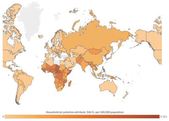
Figure 1.
Household air pollution attributed DALYs per 100,000 people [16].
2.2. Evaluation Framework
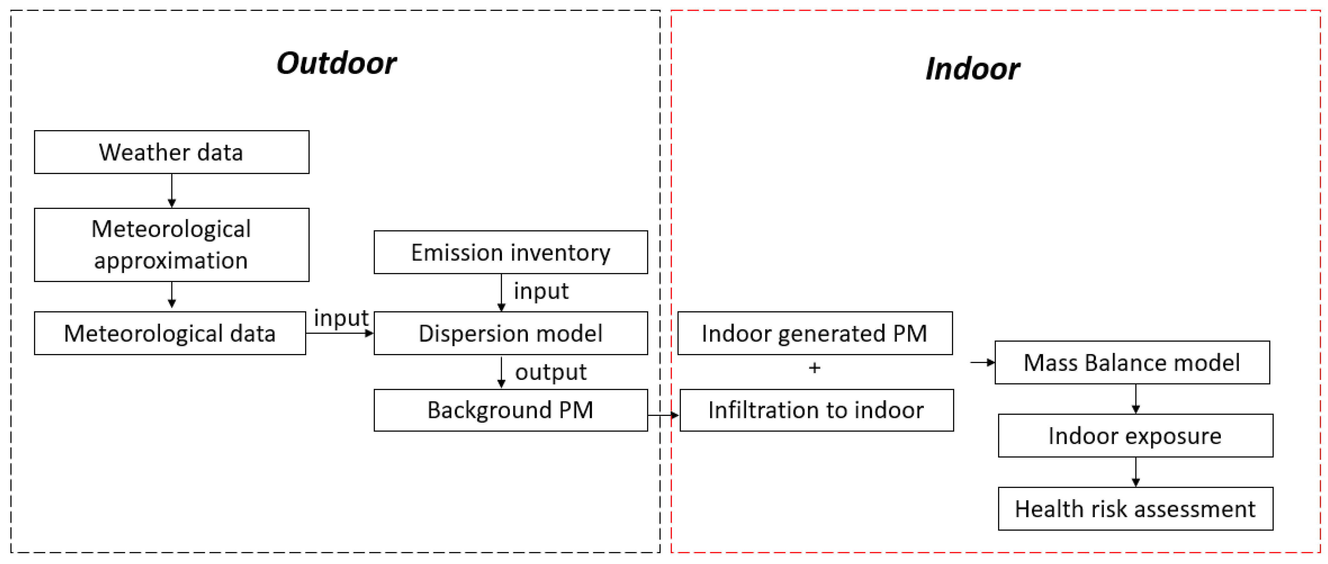
The schematic of the study process is shown in Figure 2. The study is divided into the estimation of outdoor and indoor air quality. For the outdoor air quality study, meteorological parameters such as temperature, wind speed, direction, and cloud cover are required. These required micrometeorological parameters for the dispersion model inputs are derived from routine weather data [18,19]. Integrating the dispersion model with a meteorological preprocessing approximation is a good alternative when the field measurements are not available. The approximation details, together with field validation, are described in the Supplementary Material. Figure S1 shows a good agreement of the measured friction velocity with the approximation model output. A dispersion model is then deployed to quantify outdoor pollutant distribution. Such outdoor pollutants near the household are the infiltration source to the indoor environment. The indoor generated PM2.5 is from indoor fugitive emissions. The infiltrated and the indoor-generated PM2.5, combine to form indoor pollution. Finally, a US EPA health risk assessment methodology [20] is utilized to quantify the potential dose and risk quotient for long-term exposure to such pollutants.
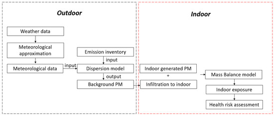
Figure 2.
Analysis flow.
2.3. Dispersion Model
Dispersion models are effective, widely utilized tools to evaluate atmospheric pollution level when field measurements are not available. Such models have been utilized to quantify pollution emitted from different sources, such as cooking, traffic, and industry [17,21,22]. The ability to isolate emission sources, thus targeting the sole effect of one possible source, can inform source management and relevant policymaking. Most of the plume models do not consider complex effects of obstacles such as buildings on the dispersion of pollutants in urban or suburban areas [23]. The current study compares AERMOD with the Quick Urban and Industrial Complex (QUIC) results to examine the influence of building morphology. QUIC accommodates building influences, rapidly enables detailed modeling of the flow field around buildings, and applies this generated wind field in a particle dispersion model. The simulation results are utilized to quantify the neighborhood infiltration because it estimates pollution dispersion in the vicinity of the buildings. AERMOD is extensively used for regulatory purposes and plays a substantial role in decision making [24]. AERMOD does not explicitly solve the flow features in the vicinity of obstacles, but accounts for obstacles through a Plume Rise Model Enhancements (PRIME) model. The current analysis compares neighborhood pollution results using both approaches. The comparison of point source dispersion among Gaussian, QUIC, and water channel evaluation is presented in Figure S2. And the comparison of contours for the outdoor emission estimation of AERMOD output with QUIC output is given in Figure S3.
QUIC has broad applications, primarily in modeling wind flow and dispersion patterns in urban or suburban areas, providing building-scale results that can show pollutant concentrations and their interaction with eddies in the built environment [23,25]. QUIC is a fast-response dispersion model that is comprised of a wind field model QUIC-URB and a dispersion model QUIC-PLUME. The flow patterns modeled by QUIC-URB have been validated with USEPA wind tunnel measurements [26]. QUIC-PLUME has also been validated through many experiments and modeling comparisons. For example, Zajic et al. compared QUIC-PLUME output to a Gaussian plume model output at different atmospheric stability, with the results being in good agreement for unstable and neutral atmospheric stabilities [27].
AERMOD was developed by the U.S. Environmental Protection Agency (EPA) in conjunction with the American Meteorological Society (AMS) to incorporate scientific advances into a dispersion model for regulatory applications [28]. AERMOD is a regulatory model with superior performance to other models in a 17 field study databases [29]. Many studies have integrated meteorological preprocessing to estimate AERMOD required inputs. Kumar et al. integrated a weather forecast model, using data-driven predicted meteorological data as inputs [30]. The current meteorological approximation has been validated for different built environments including relatively uniform terrain, as well as urban canopies [18,31].
2.4. Indoor PM2.5
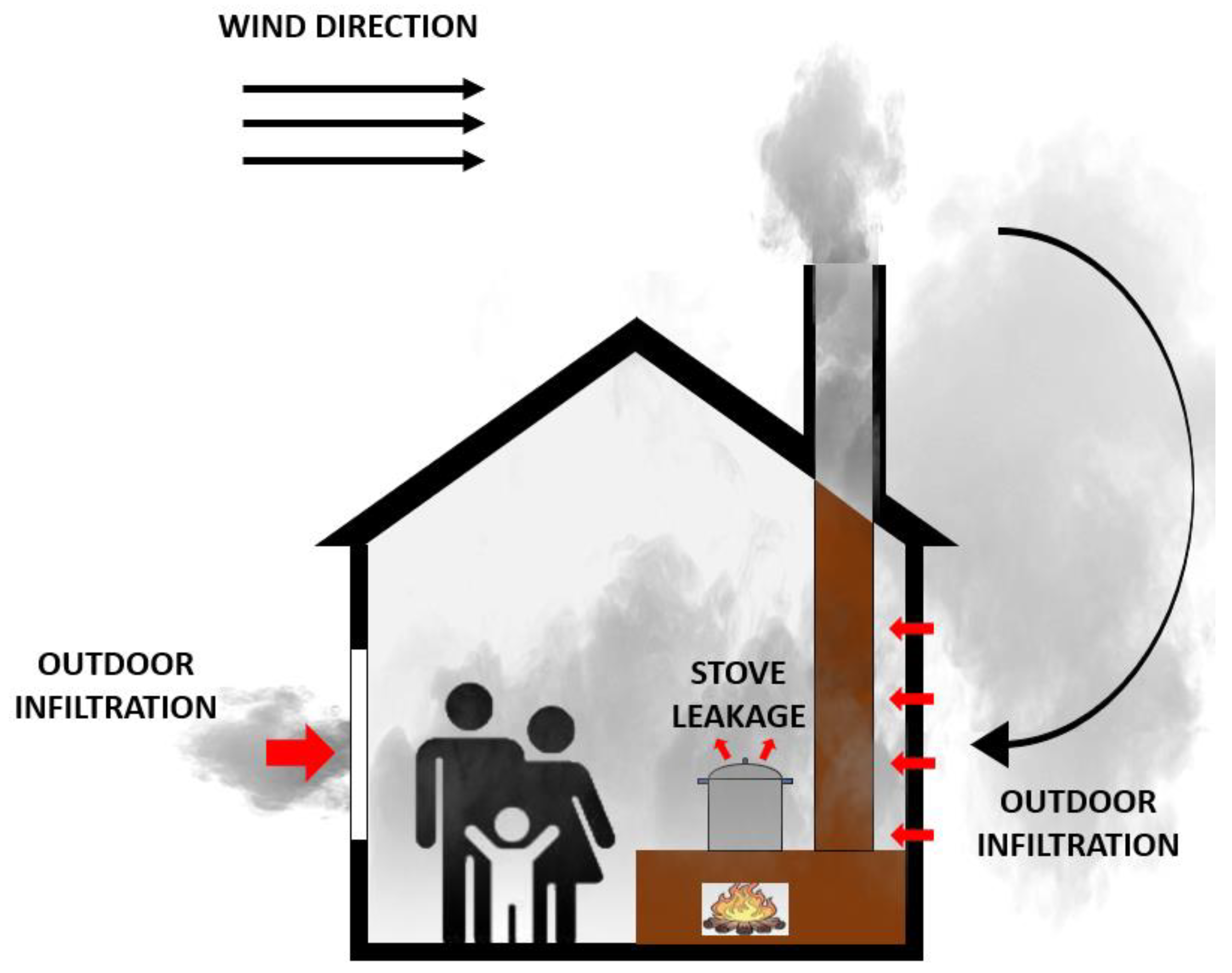
The indoor fugitive emission and infiltration of outdoor pollution are the two major sources of household pollutants (please see the schematic in Figure 3). Such external infiltration from the upstream community is determined by ventilation type, room volume, flow direction, and nature and size of openings in walls, windows, and doors. The ventilation in rural households is usually natural, wherein the leakage of airflow is through the openings in the building walls, windows, and doors. The dimensionless infiltration factor of outdoor pollution to the indoors is described by [14,32]:
where a is the air changes per hour (ACH), P is the penetration coefficient that indicates the fraction of outdoor pollutant passing indoors [33], and k is the pollutant deposition rate per hour. ACH is the rate of indoor air replacement by outdoor air. It is an important parameter that determines air ventilation in microenvironments, thus affecting indoor air exposure [34].When particles penetrate through the building envelope, gravity, diffusion, and inertial interaction are the major determinants of P. P shows a hill-shape distribution with respect to particle size, and it is assumed to be 0.8 in the study case [32]. K describes the flux of particulate matter deposited on the frames of windows, doors, walls, and other surfaces when traveling indoors and it is adapted to be 0.53 h−1 for particle size at 2.5 μm, based on experiments in six naturally ventilated houses [32].

Figure 3.
Household pollution sources from indoor fugitive emission and outdoor infiltration.
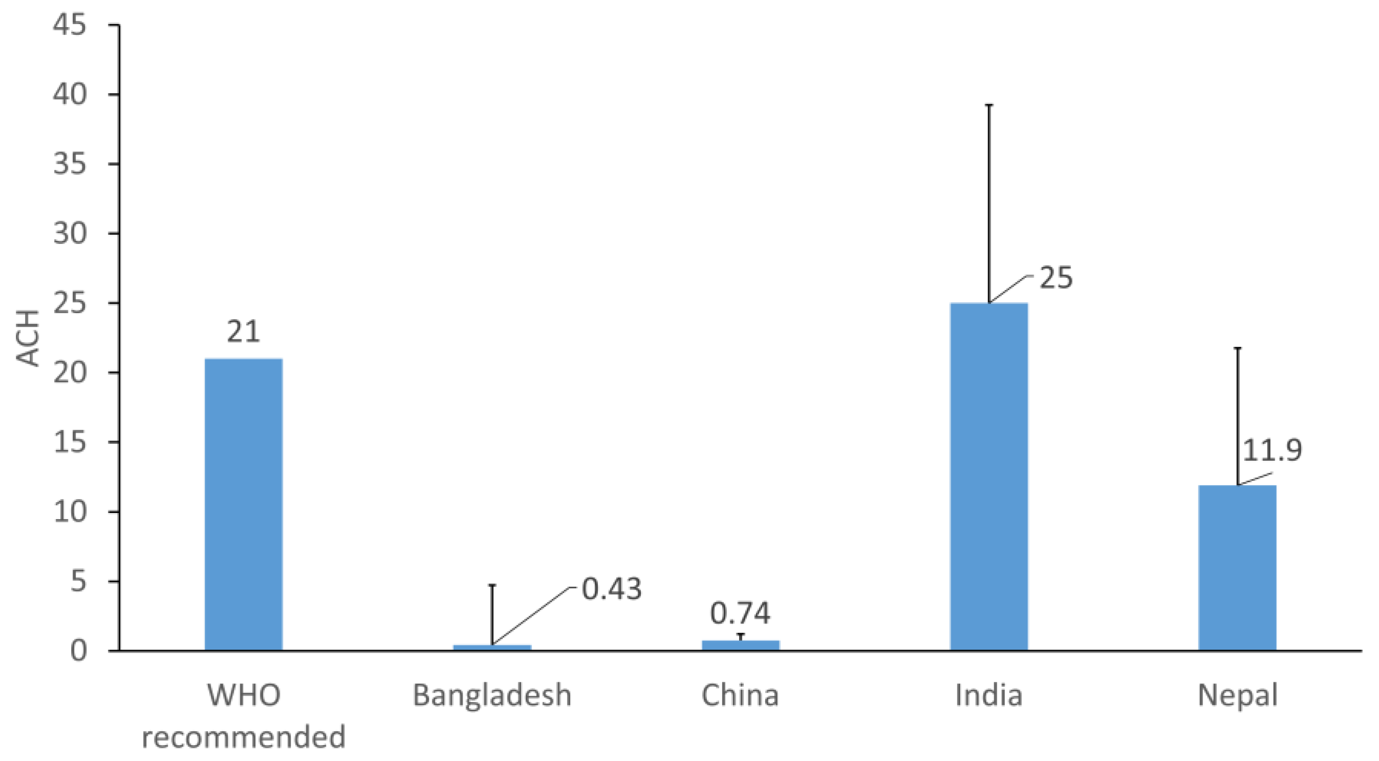
The ACH in a region can vary substantially based on the local wind speed, location, and the closing/opening of the door and windows. Figure 4 shows different ACH measured in rural areas in India [7], Bangladesh [34], China [35], and Nepal [36]. When the windows are closed, the ventilation is solely dependent on the leakage through gaps. The Literature states that the ACH in such conditions is around 1–2 for houses with solid walls. WHO suggested a default ACH of 21, for kitchens using biomass for cooking, to achieve the indoor air quality standard [37]. For current analysis, indoor pollution concentration and residents’ potential dose were estimated for ACH range of 1–25.

Figure 4.
Reference rural air changes per hour in different regions.
Using the calculated dimensionless infiltration factor, the outdoor infiltration is then described by:
where Cout is the outdoor PM2.5 concentration in μg/m3, which is obtained from the dispersion model output.
Computational Fluid Dynamic (CFD) models are at times utilized for indoor air quality modeling [38,39]. In contrast, the current study deployed a computationally inexpensive single zone mass balance model [40] to estimate the indoor generated PM2.5 concentration, which is described by:
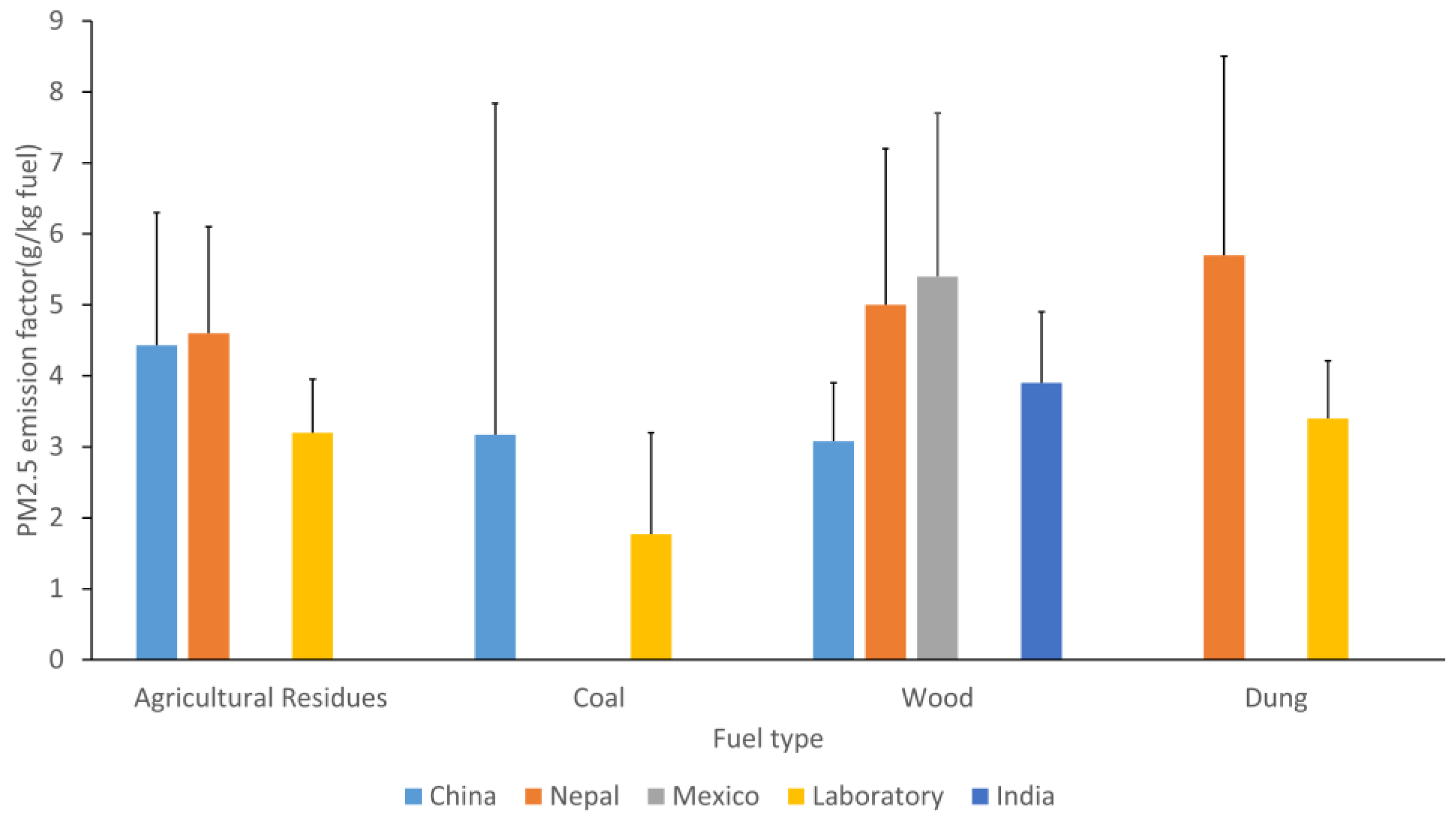
where V is the kitchen volume, which is ~40 m3 for multiple regions [41]. S is the indoor source emission rate in μg/h. In reality, the emission rate measurements vary widely, based on factors such as experimental methodology, combustion facilities, and fuel properties [8]. The indoor fugitive emission is around 2–5% of the total emission, based on the laboratory experiments, as well as field measurements [8,10,41]. Household energy needs are met mainly by biomass fuels, including crop residues, wood, coal, etc. Usage of different types of fuels impact the overall emission levels. Figure 5 presents the PM2.5 emission factor (EF) of different fuel types, in the laboratory [42] and in field, in different regions including China [8], Nepal [42], Mexico [43], and India [42]. For the same type of fuel, the EF differences may be due to factors such as fuel shape, moisture content, and the stove differences. With the different emission factors, one can estimate the emission inventory based on the fuel consumption rate from the various cooking events [44].
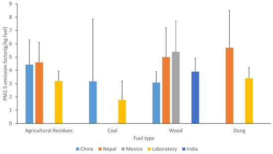
Figure 5.
Reference emission factor for different fuel types.
2.5. Health Risk Assessment
The potential dose of stove-induced PM2.5 for individuals under long-term exposure to cooking emissions is assessed using US EPA risk assessment [20]. The potential dose (I) in μg/kg·day of PM2.5 can be quantified as [15,45,46]:
where CA is the concentration of PM2.5 in μg/m3. ET is the exposure time in h/day, which in this study, is assumed to be 3 h exposure per day [47]. EF is the exposure frequency (days/year). ED is the exposure duration in the study period. AT is the average time of exposure in a day, which is ED × 365. BW is the body weight (kg). IR is the inhalation rate (m3/h), which represents the volume of air inhaled over a specified timeframe. The inhalation rates are typically indexed to activity levels. The inhalation rate for different age groups, segregated by gender and the average body weight, is referred from the EPA Exposure Factors Handbook [48]. Note that for the male gender, the potential dose results are very similar, within 2–7%. For brevity, here we present only results calculated using available female parameters, as in many rural locations, the primary coking activities are carried out by women. Under moderate activity levels, for age groups from 0.5–3, 3–10, and 10–18 years old, the average body weight is 11 kg, 23 kg, and 50 kg, and the average inhalation rate is 0.6 m3/h, 0.9 m3/h, and 1.26 m3/h, respectively, while for the adult age groups from 18–30, 30–60, and above 60 years old, the average body weight is 62 kg, 68 kg, and 67 kg, and the average inhalation rate is 1.32 m3/h, 1.32 m3/h, and 1.2 m3/h, respectively.
The risk quotient is often used to inform the health implications due to pollutant exposure. The risk quotient is described by:
where RfD is the reference dose of PM2.5 (μg/kg·day) and represents the safe average daily dose. RfD is calculated from Equation (4), with a reference concentration of 5 μg/m3. If RQ < 1, the exposure is not considered adverse to public health; if RQ > 1, the exposure is considered detrimental to public health.
3. Results
3.1. Outdoor Pollution Level
A case study of neighborhood pollution attributed to chimney vented PM2.5 emissions is conducted using QUIC model, with a wind speed of 2 m/s (at 10 m height) and a south-southwest wind direction. The QUIC modeling results of ambient PM2.5 pollution during the steady cooking state is shown in Figure 6. The channeling effect caused by wind flow encountering the building obstacles will lead to accumulation of PM2.5 in the building wakes [23]. The QUIC model enables the detection of severely impacted regions, considering the building morphology. A typical rural village consists of regions with different building densities. In each of these building densities, the neighborhood pollution level varies because the effects of trapping PM2.5 near buildings differ. As indicated in Figure 6, the maximum ground level concentration occurred in the high building density region. Although the prevailing wind is from the south-southwest, the buildings in the high-density region substantially disturb the flow and consequently, distribute the emissions in different directions, while in the low-density region, the rarely disturbed flow quickly dilutes PM2.5.
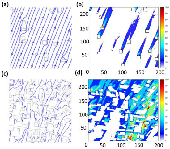
Figure 6.
Outdoor dispersion modeling results: (a,c) flow trajectory for a low- and high-density region, respectively; (b,d). PM2.5 mass concentration distribution in a low- and high-density region, respectively.
The current analysis used an emission rate of 52 mg/min for the outdoor pollution modeling based on field measurements, with 96% of total emissions from chimneys [41]. The mean PM2.5 in the high building density region is 21.2 ± 4.26 μg/m3. The mean PM2.5 in the low building density region is 4.57 ± 2.8 μg/m3. The high-density area is more impacted, regardless of the wind direction, due to the building density. Hence, this region has the highest level of PM2.5 in the communities.
Other factors, such as seasonal relative humidity, temperature, and precipitation, also play a significant role in outdoor pollution dispersion across seasons [49]. In the Brazilian rainforest, during the dry season, exposures to PM2.5 can be 6 times higher than during the rainy season [15]. This lower exposure can be attributed to the leaching of air pollution to the ground as a result of higher precipitation in the rainy season [50].
3.2. Indoor Pollution Level
Instead of completely switching to clean fuel, which may be impractical, many studies have also recommended alternative actions to reduce household air pollution and exposure. Other studies have also recommended alternative actions to reduce household air pollution and exposure, such as increasing the natural ventilation rates [51]. Combining chimneys with improved combustion chambers in stoves can also result in substantially reduced overall emissions, although chimney maintenance is necessary to maintain these reductions [41]. Leakage emissions from well-maintained stoves were shown to be substantially lower than from those in need of repair, such as the filling of cracks and the cleaning of chimneys [52].
Despite the up to 90% reductions in indoor air concentrations of PM2.5 associated with the installation of chimneys [53], fugitive concentration, combined with outdoor infiltrations, still contributes to poor indoor air quality. The indoor pollutant concentration is determined by the fugitive emission rates, room volume, particulate matter decay rate, and the infiltration of pollution from outdoors due to ventilation. Figure 7 shows the modeled indoor generated PM2.5 mass concentrations during 1 h of cooking under different air exchange rates, incorporating contributions of both fugitive emissions and neighborhood infiltration for high-packing density. The fugitive emission rate ranges from 0.26–2.6 mg/min, based on direct field measurements in different regions [8,10,41,54]. The ACH ranges from 1–25 h−1, from poor ventilated cases, to WHO default ventilation rates for ISO tiers.
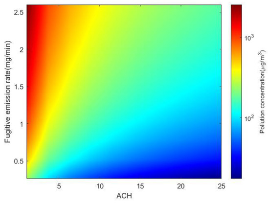
Figure 7.
Indoor PM2.5 concentrations under different ACH incorporating fugitive emission and neighborhood infiltration for a high-packing density neighborhood.
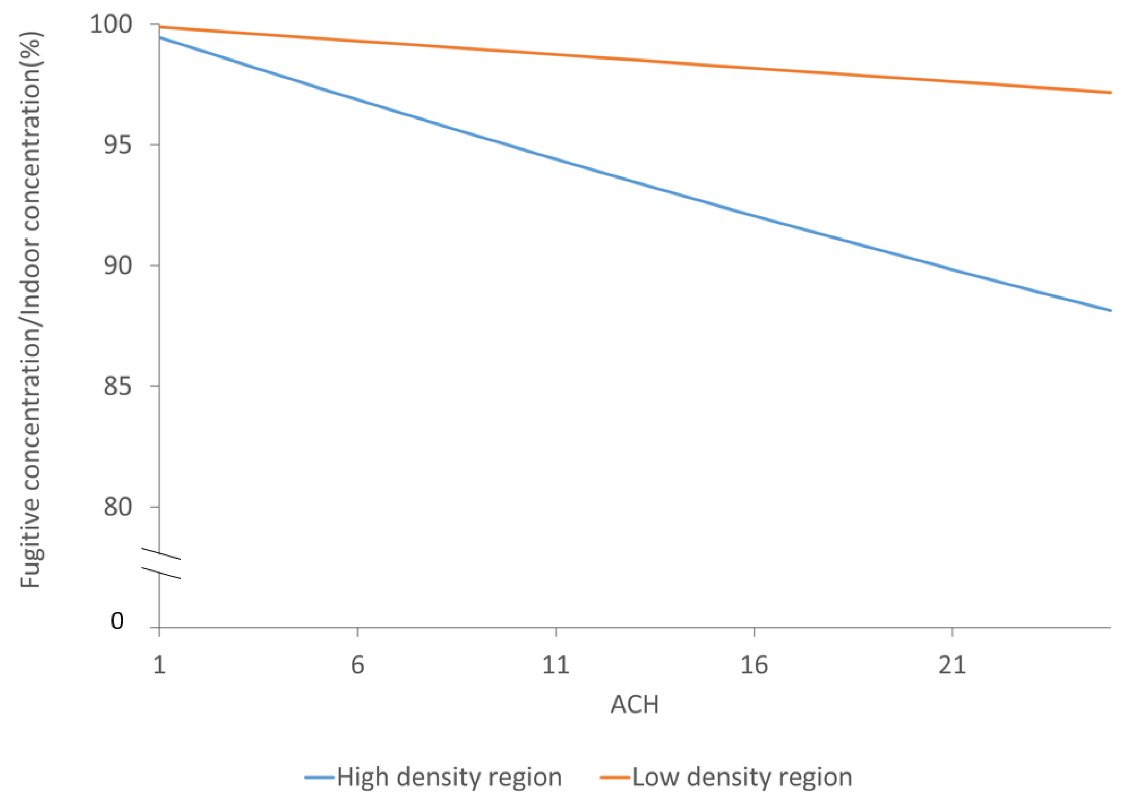
Infiltration of pollution from outdoors consists of both neighborhood pollution and regional background PM2.5. The neighborhood pollution contribution to indoor concentrations depends on the packing density of upstream homes. Figure 8 shows the percentage of fugitive contribution to the total indoor air PM2.5 concentrations. At 25 ACH, for homes in the high packing density area, the indoor generated PM2.5 accounts for 90% of the total concentration, while for a low packing density region, the number is 98%.
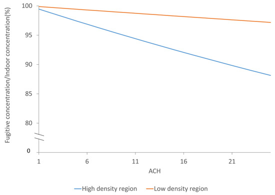
Figure 8.
Contribution of fugitive emission to indoor air PM2.5 concentrations.
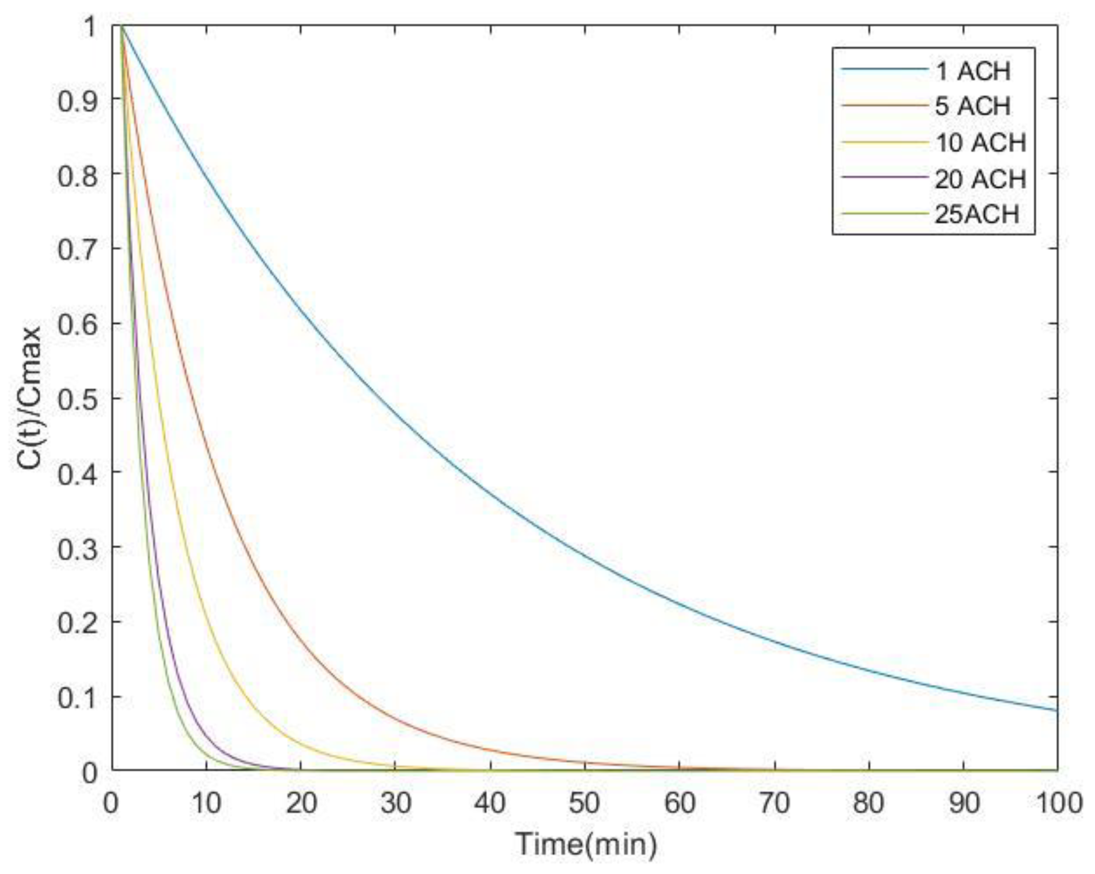
After the cooking concludes, the decay trend of the relative mass concentration (C(t)/Cmax) under ACH = 1, 5, 10, 20, and 25 are shown in Figure 9. Studies indicated that the building characteristics, including ventilation, orientation, the morphology of the streets, wall construction, eave spaces, open–closed windows, etc., dominate the air exchange rate [50,55].
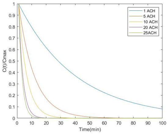
Figure 9.
Influence of different ACHs on relative indoor concentration decay trend after steady cooking events.
This case study uses a fugitive emission rate of 2.1 mg/min, which is directly measured in rural Mexico using nested hoods to capture all emissions [41]. Even at the recommended 21 ACH, the indoor pollution concentration during the 1 h steady cooking event is 174 μg/m3, with fugitive emissions contributing 90% to indoor concentrations. The corresponding 24 h average PM2.5 level is ~21 μg/m3 under the assumption that each household conducts 3 h cooking each day [47]. This exceeds the 2021 WHO air quality guideline of 15 μg/m3 for 24 h.
PM2.5 concentration levels in different rooms can be significantly lower than in other rooms [56] and can vary by season [49]. Zuk et al. found that the kitchen concentrations were two times that of other rooms [56]. In addition, in many homes cooking-generated PM2.5 may readily spread to the adjacent rooms in the house [49,57]. Since people spend the most time in bedrooms and living rooms, having a separate kitchen can help reduce exposures, although, room ventilation and location relative to the kitchen have been reported to impact the PM2.5 level in the room [58]. Behavior changes, such as opening doors and windows [59] and the use of extraction fans, may also reduce indoor concentrations.
3.3. Potential Dose Assessment
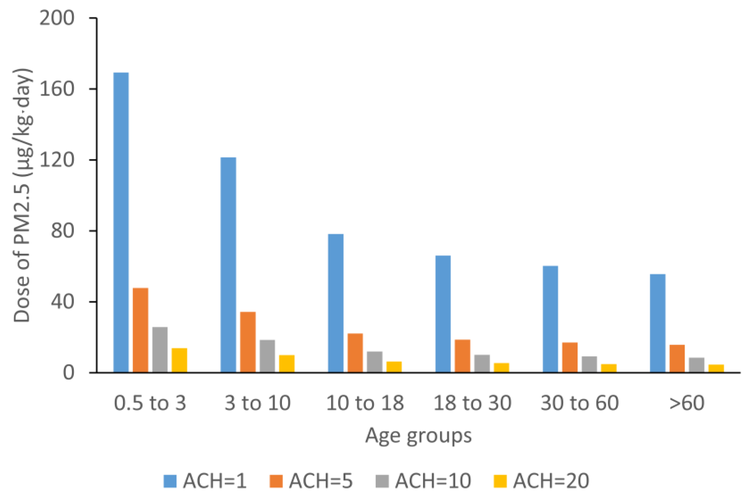
The inhaled dose is determined by individual behaviors and the distance from the emission source. A number of studies have shown that personal exposures are ~50% of indoor kitchen concentrations [52,60], as personal exposures include time spent away from the kitchen in other environments. Figure 10 shows the potential dose estimated under personal exposure. The risk quotient (RQ) for exposed residents is 26, 7.93, 3.96, and 2.19 under 1, 5, 10, and 20 ACH, respectively. This shows that even under high ventilation rates, household emissions moderately contribute to total chronic exposure and may induce respiratory health problems. Besides, the potential intake of pollutants from cooking activity is high, and thus, the long-term exposure can significantly impact individuals who perform the cooking.
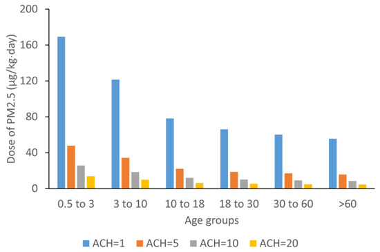
Figure 10.
Case study of potential dose of PM2.5 for different age groups under different ventilation parameters.
In general, potential PM2.5 doses decreased with age groups, and children under 3 years had the highest potential dose, in agreement with other studies [15,50], because younger children are more active and breathe more per unit of body weight.
A study of chimney stove impact conducted over a period of 12 months by Chakraborty et al. found that the median value of PM2.5 RQ was 1.63 [61]. Although the utilization of a chimney stove has adverse health effects, the results show a lower PM2.5 potential dose compared to that from a traditional open fire, for which the observed RQ can be as high as 5.57 [61].
Single-zone models tend to overestimate concentrations, as the model assumes a well-mixed environment, which may attribute to the discrepancies in the calculated and measured concentration [62]. The overestimation of potential dose can thus be a limitation of this approach.
4. Conclusions
The aim of this study is to provide a full-cycle analysis integrating air quality models, infiltration models, and risk assessment models to better understand the impacts of neighborhood pollution and stove fugitive emissions on the potential dose. The main conclusions of this study are:
- PM2.5 pollutants tend to accumulate in the wake of buildings, and the pollutant infiltration can contribute significantly to poor indoor air quality. The major contributor to indoor pollution, however, is fugitive emissions from cooking stoves.
- The contribution of chimney stoves to infiltration increases with higher packing densities and may contribute to indoor pollutant concentrations.
- Indoor concentrations from chimney stoves exceed WHO air quality guideline values for PM2.5. The associated health risk assessment shows that the risk quotient (RQ) is 2.19, despite good ventilation conditions.
Supplementary Materials
The following supporting information can be downloaded at: https://www.mdpi.com/article/10.3390/su15075676/s1, Figure S1: Comparison of meteorological approximation model output and field measurement; Figure S2: Comparison of point source dispersion among Gaussian, QUIC, and water channel evaluation; Figure S3: Comparison of (left) AERMOD output with (right) QUIC output for one-hour outdoor emission estimation. References [18,19,63,64,65] are cited in the supplementary materials.
Author Contributions
Conceptualization, Y.H., S.R.N., R.D.E. and M.P.; data curation, Y.H. and S.R.N.; formal analysis, Y.H. and S.R.N.; investigation, Y.H. and S.R.N.; software, Y.H. and S.R.N.; validation, Y.H. and S.R.N.; visualization, Y.H. and S.R.N.; methodology, Y.H. and S.R.N.; funding acquisition, R.D.E.; project administration, R.D.E. and M.P.; supervision, M.P. and R.D.E.; writing—original draft, Y.H. and S.R.N.; writing—review and editing, Y.H., S.R.N., R.D.E. and M.P. All authors have read and agreed to the published version of the manuscript.
Funding
This work was funded by Clean Stacking Options and Regional IAP Scenarios for Rural Mexico, NIH-5585744.
Institutional Review Board Statement
Not applicable.
Informed Consent Statement
Not applicable.
Data Availability Statement
Not applicable.
Acknowledgments
We are grateful to the Los Alamos National Laboratory for providing the QUIC model under license number: LIC-20-04147. Special thanks to Hannah Lee, Rebecca Albano, and Arthor Bernal for running the QUIC simulation.
Conflicts of Interest
The authors declare no conflict of interest.
References
- Chafe, Z.A.; Brauer, M.; Klimont, Z.; Van Dingenen, R.; Mehta, S.; Rao, S.; Riahi, K.; Dentener, F.; Smith, K.R. Household cooking with solid fuels contributes to ambient PM2.5air pollution and the burden of disease. Environ. Health Perspect. 2015, 122, 1314–1320. [Google Scholar] [CrossRef] [PubMed]
- Pilishvili, T.; Loo, J.D.; Schrag, S.; Stanistreet, D.; Christensen, B.; Yip, F.; Nyagol, R.; Quick, R.; Sage, M.; Bruce, N. Effectiveness of six improved cookstoves in reducing household air pollution and their acceptability in rural western Kenya. PLoS ONE 2016, 11, e0165529. [Google Scholar] [CrossRef] [PubMed]
- García-Frapolli, E.; Schilmann, A.; Berrueta, V.M.; Riojas-Rodríguez, H.; Edwards, R.D.; Johnson, M.; Guevara-Sanginés, A.; Armendariz, C.; Masera, O. Beyond fuelwood savings: Valuing the economic benefits of introducing improved biomass cookstoves in the Purépecha region of Mexico. Ecol. Econ. 2010, 69, 2598–2605. [Google Scholar] [CrossRef]
- McCreanor, J.; Cullinan, P.; Nieuwenhuijsen, M.J.; Stewart-Evans, J.; Malliarou, E.; Jarup, L.; Harrington, R.; Svartengren, M.; Han, I.-K.; Ohman-Strickland, P.; et al. Respiratory Effects of Exposure to Diesel Traffic in Persons with Asthma. N. Engl. J. Med. 2007, 357, 2348–2358. [Google Scholar] [CrossRef]
- World Health Organization. Household Air Pollution. Available online: https://www.who.int/news-room/fact-sheets/detail/household-air-pollution-and-health (accessed on 17 December 2022).
- Parajuli, I.; Lee, H.; Shrestha, K.R. Indoor Air Quality and ventilation assessment of rural mountainous households of Nepal. Int. J. Sustain. Built Environ. 2016, 5, 301–311. [Google Scholar] [CrossRef]
- Johnson, M.; Lam, N.; Brant, S.; Gray, C.; Pennise, D. Modeling indoor air pollution from cookstove emissions in developing countries using a Monte Carlo single-box model. Atmos. Environ. 2011, 45, 3237–3243. [Google Scholar] [CrossRef]
- Shen, H.; Luo, Z.; Xiong, R.; Liu, X.; Zhang, L.; Li, Y.; Du, W.; Chen, Y.; Cheng, H.; Shen, G.; et al. A critical review of pollutant emission factors from fuel combustion in home stoves. Environ. Int. 2021, 157, 106841. [Google Scholar] [CrossRef]
- Ruiz, V.; Masera, O. Estimating Kitchen PM 2.5 and CO Concentrations out of Stove Emissions: The Case of Mexican Plancha-Type Stoves; Universidad Nacional Autónoma de México: Morelia, Mexico, 2018. [Google Scholar]
- Shen, G.; Du, W.; Luo, Z.; Li, Y.; Cai, G.; Lu, C.; Qiu, Y.; Chen, Y.; Cheng, H.; Tao, S. Fugitive Emissions of CO and PM2.5 from Indoor Biomass Burning in Chimney Stoves Based on a Newly Developed Carbon Balance Approach. Environ. Sci. Technol. Lett. 2020, 7, 128–134. [Google Scholar] [CrossRef]
- Lim, M.; Myagmarchuluun, S.; Ban, H.; Hwang, Y.; Ochir, C.; Lodoisamba, D.; Lee, K. Characteristics of indoor pm2.5 concentration in gers using coal stoves in ulaanbaatar, mongolia. Int. J. Environ. Res. Public Health 2018, 15, 2524. [Google Scholar] [CrossRef]
- Pope, C.A.; Dockery, D.W. Health effects of fine particulate air pollution: Lines that connect. J. Air Waste Manag. Assoc. 2006, 56, 709–742. [Google Scholar] [CrossRef]
- Laumbach, R.J.; Kipen, H.M. Respiratory health effects of air pollution: Update on biomass smoke and traffic pollution. J. Allergy Clin. Immunol. 2012, 129, 3–11. [Google Scholar] [CrossRef] [PubMed]
- Breen, M.S.; Schultz, B.D.; Sohn, M.D.; Long, T.; Langstaff, J.; Williams, R.; Isaacs, K.; Meng, Q.Y.; Stallings, C.; Smith, L. A review of air exchange rate models for air pollution exposure assessments. J. Expo. Sci. Environ. Epidemiol. 2014, 24, 555–563. [Google Scholar] [CrossRef] [PubMed]
- De Oliveira, B.F.A.; Ignotti, E.; Artaxo, P.; Do Nascimento Saldiva, P.H.; Junger, W.L.; Hacon, S. Risk assessment of PM2.5 to child residents in Brazilian Amazon region with biofuel production. Environ. Health A Glob. Access Sci. Source 2012, 11, 64. [Google Scholar] [CrossRef] [PubMed]
- World Health Organization. Household Air Pollution Attributable Dalys. Available online: https://www.who.int/data/gho/data/indicators/indicator-details/GHO/household-air-pollution-attributable-dalys (accessed on 16 December 2022).
- Edwards, R.; Princevac, M.; Weltman, R.; Ghasemian, M.; Arora, N.K.; Bond, T. Modeling emission rates and exposures from outdoor cooking. Atmos. Environ. 2017, 164, 50–60. [Google Scholar] [CrossRef]
- Qian, W.; Princevac, M.; Venkatram, A. Using temperature fluctuation measurements to estimate meteorological inputs for modelling dispersion during convective conditions in urban areas. Bound.-Layer Meteorol. 2010, 135, 269–289. [Google Scholar] [CrossRef][Green Version]
- Holtslag, A.A.M.; Van Ulden, A.P. A simple scheme for daytime estimates of the surface fluxes from routine weather data. J. Appl. Meteorol. Climatol. 1983, 22, 517–529. [Google Scholar] [CrossRef]
- Means, B. Risk-Assessment Guidance for Superfund. Volume 1. Human Health Evaluation Manual. Part A. Interim Report (Final); Environmental Protection Agency: Washington, DC, USA, 1989.
- Venkatram, A.; Isakov, V.; Thoma, E.; Baldauf, R. Analysis of air quality data near roadways using a dispersion model. Atmos. Environ. 2007, 41, 9481–9497. [Google Scholar] [CrossRef]
- López, M.T.; Zuk, M.; Garibay, V.; Tzintzun, G.; Iniestra, R.; Fernández, A. Health impacts from power plant emissions in Mexico. Atmos. Environ. 2005, 39, 1199–1209. [Google Scholar] [CrossRef]
- Brown, M.J.; Williams, M.D.; Nelson, M.A.; Werley, K.A. QUIC Transport and Dispersion Modeling of Vehicle Emissions in Cities for Better Public Health Assessments. Environ. Health Insights 2015, 9s1, EHI-S15662. [Google Scholar] [CrossRef]
- Patiño, W.R.; Duong, V.M. Intercomparison of Gaussian Plume Dispersion Models Applied to Sulfur Dioxide Emissions from a Stationary Source in the Suburban Area of Prague, Czech Republic. Environ. Model. Assess. 2021, 27, 119–137. [Google Scholar] [CrossRef]
- Bowker, G.E.; Gillette, D.A.; Bergametti, G.; Marticorena, B. Modeling flow patterns in a small vegetated area in the northern Chihuahuan Desert using QUIC (Quick Urban & Industrial Complex). Environ. Fluid Mech. 2006, 6, 359–384. [Google Scholar] [CrossRef]
- Bowker, G.E.; Perry, S.G.; Heist, D.K. A comparison of airflow patterns from the QUIC model and an atmospheric wind tunnel for a two-dimensional building array and a multi-city block region near the World Trade Center site. Presented at the 5th Symposium on the Urban Environment, Vancouver, BC, Canada, 23–27 August 2004. [Google Scholar]
- Brown, M.J. Quick Urban and Industrial Complex (QUIC) CBR Plume Modeling System: Validation-Study Document; Los Alamos National Lab. (LANL): Los Alamos, NM, USA, 2018.
- Cimorelli, A.J.; Perry, S.G.; Venkatram, A.; Weil, J.C.; Paine, R.J.; Wilson, R.B.; Lee, R.F.; Peters, W.D.; Brode, R.W. AERMOD: A dispersion model for industrial source applications. Part I: General model formulation and boundary layer characterization. J. Appl. Meteorol. 2005, 44, 682–693. [Google Scholar] [CrossRef]
- Perry, S.G.; Cimorelli, A.J.; Paine, R.J.; Brode, R.W.; Weil, J.C.; Venkatram, A.; Wilson, R.B.; Lee, R.F.; Peters, W.D. AERMOD: A Dispersion model for industrial source applications. Part II: Model performance against 17 field study databases. J. Appl. Meteorol. 2005, 44, 694–708. [Google Scholar] [CrossRef]
- Kumar, A.; Dikshit, A.K.; Patil, R.S. Use of simulated and observed meteorology for air quality modeling and source ranking for an industrial region. Sustainability 2021, 13, 4276. [Google Scholar] [CrossRef]
- Wiernga, J. Representative roughness parameters for homogeneous terrain. Bound.-Layer Meteorol. 1993, 63, 323–363. [Google Scholar] [CrossRef]
- Chao, C.Y.H.; Wan, M.P.; Cheng, E.C.K. Penetration coefficient and deposition rate as a function of particle size in non-smoking naturally ventilated residences. Atmos. Environ. 2003, 37, 4233–4241. [Google Scholar] [CrossRef]
- Liu, D.L.; Nazaroff, W.W. Modeling pollutant penetration across building envelopes. Atmos. Environ. 2001, 35, 4451–4462. [Google Scholar] [CrossRef]
- Das, D.; Moynihan, E.; Nicas, M.; McCollum, E.D.; Ahmed, S.; Roy, A.D.; Chowdhury, N.; Hanif, A.A.M.; Babik, K.R.; Baqui, A.H.; et al. Estimating residential air exchange rates in rural Bangladesh using a near field-far field model. Build. Environ. 2021, 206, 108325. [Google Scholar] [CrossRef]
- Zhou, B.; Zhao, B.; Zhou, W. Characterizing PM2.5 concentration and air exchange rates in Chinese rural kitchens: A field study. In Proceedings of the 10th International Healthy Buildings Conference, Brisbane, Australia, 8–12 July 2012; Volume 1, pp. 260–261. [Google Scholar]
- Soneja, S.I.; Tielsch, J.M.; Curriero, F.C.; Zaitchik, B.; Khatry, S.K.; Yan, B.; Chillrud, S.N.; Breysse, P.N. Determining particulate matter and black carbon exfiltration estimates for traditional cookstove use in rural nepalese village households. Environ. Sci. Technol. 2015, 49, 5555–5562. [Google Scholar] [CrossRef]
- ISO. Technical Report ISO/TR Solutions—Harmonized Laboratory Cookstoves Based on Laboratory Testing; ISO: Geneva, Switzerland, 2018; Volume 2018. [Google Scholar]
- Nishandar, S.R.; He, Y.; Princevac, M.; Edwards, R.D. Fate of Exhaled Droplets From Breathing and Coughing in Supermarket Checkouts and Passenger Cars. Environ. Health Insights 2023, 17. [Google Scholar] [CrossRef]
- Mohammadi, M.; Calautit, J. Impact of Ventilation Strategy on the Transmission of Outdoor Pollutants into Indoor Environment Using CFD. Sustainability 2021, 13, 10343. [Google Scholar] [CrossRef]
- Leary, C.O.; Jones, B.; Leary, C.O.; Jones, B. A Method to Measure Emission Rates of PM2.5s from Cooking A Method to Measure Emission Rates of PM 2.5 s from Cooking. In Proceedings of the 38th Air Infiltration and Ventilation Centre Conference, Nottingham, UK, 13–14 September 2017. [Google Scholar]
- Ruiz-García, V.M.; Edwards, R.D.; Ghasemian, M.; Berrueta, V.M.; Princevac, M.; Vázquez, J.C.; Johnson, M.; Masera, O.R. Fugitive Emissions and Health Implications of Plancha-Type Stoves. Environ. Sci. Technol. 2018, 52, 10848–10855. [Google Scholar] [CrossRef] [PubMed]
- Edwards, R.; Bond, T.; KR, S. Characterization of emissions from small, variable solid fuel combustion sources for determining global emissions and climate impact. Final Proj. 2017, 83503601, 1–69. [Google Scholar]
- Johnson, M.; Edwards, R.; Alatorre Frenk, C.; Masera, O. In-field greenhouse gas emissions from cookstoves in rural Mexican households. Atmos. Environ. 2008, 42, 1206–1222. [Google Scholar] [CrossRef]
- Du, W.; Zhuo, S.; Wang, J.; Luo, Z.; Chen, Y.; Wang, Z.; Lin, N.; Cheng, H.; Shen, G.; Tao, S. Substantial leakage into indoor air from on-site solid fuel combustion in chimney stoves. Environ. Pollut. 2021, 291, 118138. [Google Scholar] [CrossRef]
- Bixapathi, B.; Reddy, P.V.V.; Rao, M.S.; Raghavendra, T. Health risk assessment of four important ambient air pollutants in Hyderabad. NVEO-Nat. Volatiles Essent. Oils J. 2021, 8, 9925–9935. [Google Scholar]
- de Souza Silva, P.R.; Ignotti, E.; de Oliveira, B.F.A.; Junger, W.L.; Morais, F.; Artaxo, P.; Hacon, S. High risk of respiratory diseases in children in the fire period in Western Amazon. Rev. Saude Publica 2016, 50, 29. [Google Scholar] [CrossRef]
- World Health Organization. Input Data to Run Household Multiple Emission Sources and Performance Target Models. Available online: https://www.who.int/tools/input-data-to-run-household-multiple-emission-sources-and-performance-target-models (accessed on 16 December 2022).
- U.S. Environmental Protection Agency. U.S. EPA. Exposure Factors Handbook; U.S. Environmental Protection Agency: Washington, DC, USA, 2011.
- Edwards, R.D.; Liu, Y.; He, G.; Yin, Z.; Sinton, J.; Peabody, J.; Smith, K.R. Household CO and PM measured as part of a review of China’s National Improved Stove Program. Indoor Air 2007, 17, 189–203. [Google Scholar] [CrossRef]
- Kaewrat, J.; Janta, R.; Sichum, S.; Kanabkaew, T. Indoor air quality and human health risk assessment in the open-air classroom. Sustainability 2021, 13, 8302. [Google Scholar] [CrossRef]
- Pokhrel, A.K.; Bates, M.N.; Acharya, J.; Valentiner-Branth, P.; Chandyo, R.K.; Shrestha, P.S.; Raut, A.K.; Smith, K.R. PM2.5 in household kitchens of Bhaktapur, Nepal, using four different cooking fuels. Atmos. Environ. 2015, 113, 159–168. [Google Scholar] [CrossRef]
- Hartinger, S.M.; Commodore, A.A.; Hattendorf, J.; Lanata, C.F.; Gil, A.I.; Verastegui, H.; Aguilar-Villalobos, M.; Mäusezahl, D.; Naeher, L.P. Chimney stoves modestly improved Indoor Air Quality measurements compared with traditional open fire stoves: Results from a small-scale intervention study in rural Peru. Indoor Air 2013, 23, 342–352. [Google Scholar] [CrossRef] [PubMed]
- Masera, O.; Edwards, R.; Arnez, C.A.; Berrueta, V.; Johnson, M.; Bracho, L.R.; Riojas-Rodríguez, H.; Smith, K.R. Impact of Patsari improved cookstoves on indoor air quality in Michoacán, Mexico. Energy Sustain. Dev. 2007, 11, 45–56. [Google Scholar] [CrossRef]
- Jetter, J. In Stove 60-Liter Institutional Stove with Wood Fuel—Air Pollutant Emissions and Fuel Efficiency; US Environmental Protection Agency: Washington, DC, USA, 2016.
- Howard-Reed, C.; Wallace, L.A.; Ott, W.R. The effect of opening windows on air change rates in two homes. J. Air Waste Manag. Assoc. 2002, 52, 147–159. [Google Scholar] [CrossRef] [PubMed]
- Zuk, M.; Rojas, L.; Blanco, S.; Serrano, P.; Cruz, J.; Angeles, F.; Tzintzun, G.; Armendariz, C.; Edwards, R.D.; Johnson, M.; et al. The impact of improved wood-burning stoves on fine particulate matter concentrations in rural Mexican homes. J. Expo. Sci. Environ. Epidemiol. 2007, 17, 224–232. [Google Scholar] [CrossRef]
- Kim, H.; Kang, K.; Kim, T. Measurement of particulate matter (PM2.5) and health risk assessment of cooking-generated particles in the kitchen and living rooms of apartment houses. Sustainability 2018, 10, 843. [Google Scholar] [CrossRef]
- Estévez-García, J.A.; Schilmann, A.; Riojas-Rodríguez, H.; Berrueta, V.; Blanco, S.; Villaseñor-Lozano, C.G.; Flores-Ramírez, R.; Cortez-Lugo, M.; Pérez-Padilla, R. Women exposure to household air pollution after an improved cookstove program in rural San Luis Potosi, Mexico. Sci. Total Environ. 2020, 702, 134456. [Google Scholar] [CrossRef]
- Iribagiza, C.; Sharpe, T.; Coyle, J.; Nkubito, P.; Piedrahita, R.; Johnson, M.; Thomas, E.A. Evaluating the effects of access to air quality data on household air pollution and exposure—An interrupted time series experimental study in rwanda. Sustainability 2021, 13, 11523. [Google Scholar] [CrossRef]
- Pillarisetti, A.; Alnes, L.W.H.; Ye, W.; McCracken, J.P.; Canuz, E.; Smith, K.R. Repeated assessment of PM2.5 in Guatemalan kitchens cooking with wood: Implications for measurement strategies. Atmos. Environ. 2023, 295, 119533. [Google Scholar] [CrossRef]
- Chakraborty, D.; Kumar, N. Reduction in household air pollution and associated health risk: A pilot study with an improved cookstove in rural households. Clean Technol. Environ. Policy 2021, 23, 1993–2009. [Google Scholar] [CrossRef]
- Mutahi, A.W.; Borgese, L.; Marchesi, C.; Gatari, M.J.; Depero, L.E. Indoor and outdoor air quality for sustainable life: A case study of rural and urban settlements in poor neighbourhoods in kenya. Sustainability 2021, 13, 2417. [Google Scholar] [CrossRef]
- Schlichting, H.; Gersten, K. Boundary Layer Theory, 8th English edn. J. Fluid Mech. 2020, 415, 346–347. [Google Scholar]
- Wang, I.T.; Chen, P.C. Estimations of heat and momentum fluxes near the ground. Bull. Am. Meteorol. Soc. 1980, 61, 97. [Google Scholar] [CrossRef]
- Boarnet, M.G.; Edwards, R.; Princevac, M.; Wu, J.; Pan, H.; Bartolome, C.J.; Ferguson, G.; Fazl, A.; Lejano, R. Near-Source Modeling of Transportation Emissions in Built Environments Surrounding Major Arterials. Univ. Calif. Transp. Cent. Univ. Calif. Transp. Cent. Work. Papers 2009. [Google Scholar]
Disclaimer/Publisher’s Note: The statements, opinions and data contained in all publications are solely those of the individual author(s) and contributor(s) and not of MDPI and/or the editor(s). MDPI and/or the editor(s) disclaim responsibility for any injury to people or property resulting from any ideas, methods, instructions or products referred to in the content. |
© 2023 by the authors. Licensee MDPI, Basel, Switzerland. This article is an open access article distributed under the terms and conditions of the Creative Commons Attribution (CC BY) license (https://creativecommons.org/licenses/by/4.0/).


