4.1.1. Example Parameters
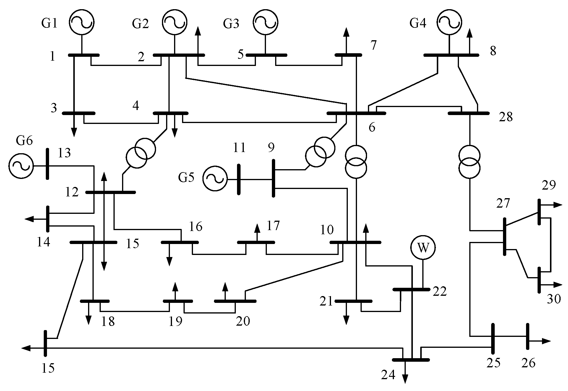
Firstly, the IEEE-30 node system connected to the wind farm is taken as an example for simulation analysis, and the system wiring diagram is shown in
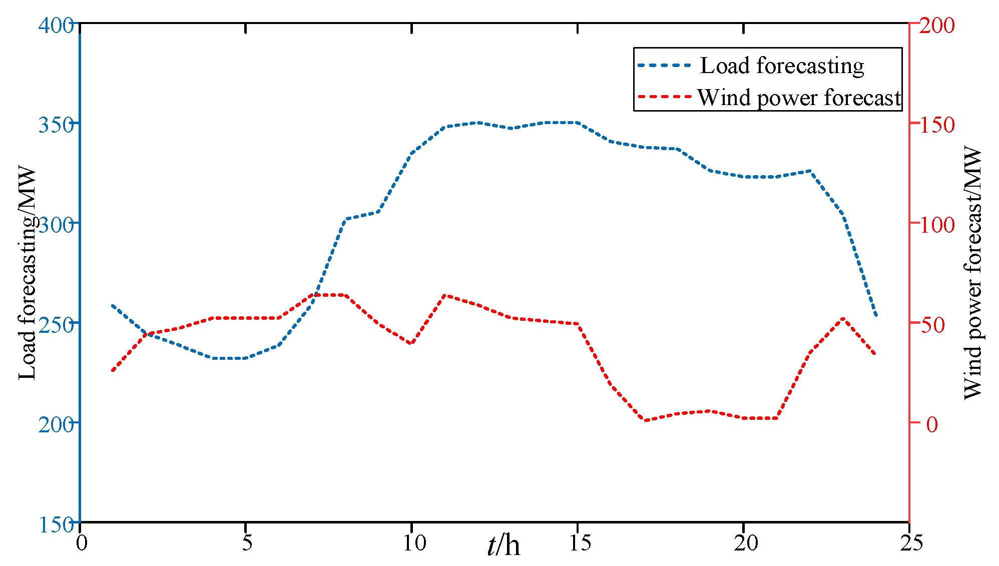
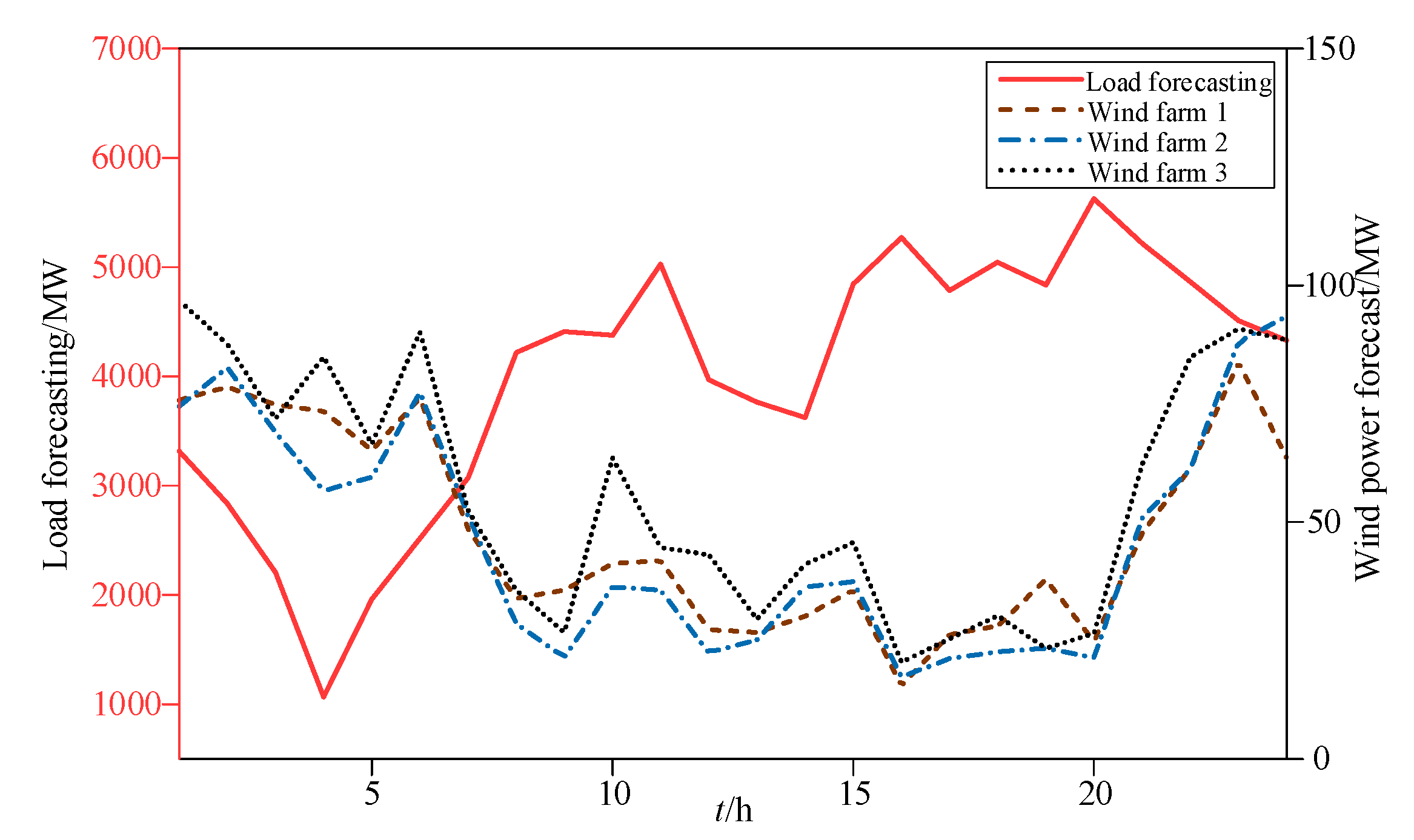
Figure 2. It includes six conventional thermal power units, which are connected to a wind farm with an installed capacity of 150 MW at 22 nodes. The predicted values of load and wind power in each period are shown in
Figure 3, and the parameters of six conventional thermal power units are shown in reference [
23]. The marginal emission factors of electricity and capacity of each unit are shown in
Table A1 of
Appendix A and other parameters are given in reference [
24]. Considering the allocation of carbon emission credits and the calculation of carbon trading costs, the time step is taken as 1 h, and the scheduling period T is 24 h [
25]. In addition, the load reserve coefficient is 0.1, and the wind power reserve coefficient is 0.14. In this chapter, the predicted carbon price of days 401 to 424 is selected to simulate the 24 h carbon trading price in the scheduling period.
The related calculation is based on MATLAB 2016a software and CPLEX 12.4, and the hardware configuration is Windows 10 64-bit operating system with CPU i5-7500 and 8G running memory [
27].
4.1.2. Simulation Results
According to the calculation method in
Section 4.2, the weights of marginal emission factor of electricity and marginal emission factor of capacity are 0.65 and 0.35 [
28], respectively, and the corresponding carbon quota coefficient of each unit is shown in
Table 1.
It can be seen from
Table 1 that thermal power unit G3 has the lowest quota coefficient, while unit G5 has the highest quota coefficient. If other factors are not taken into account [
29], the carbon emissions of the system can be reduced by giving priority to dispatching unit G3 when the system needs the same output level.
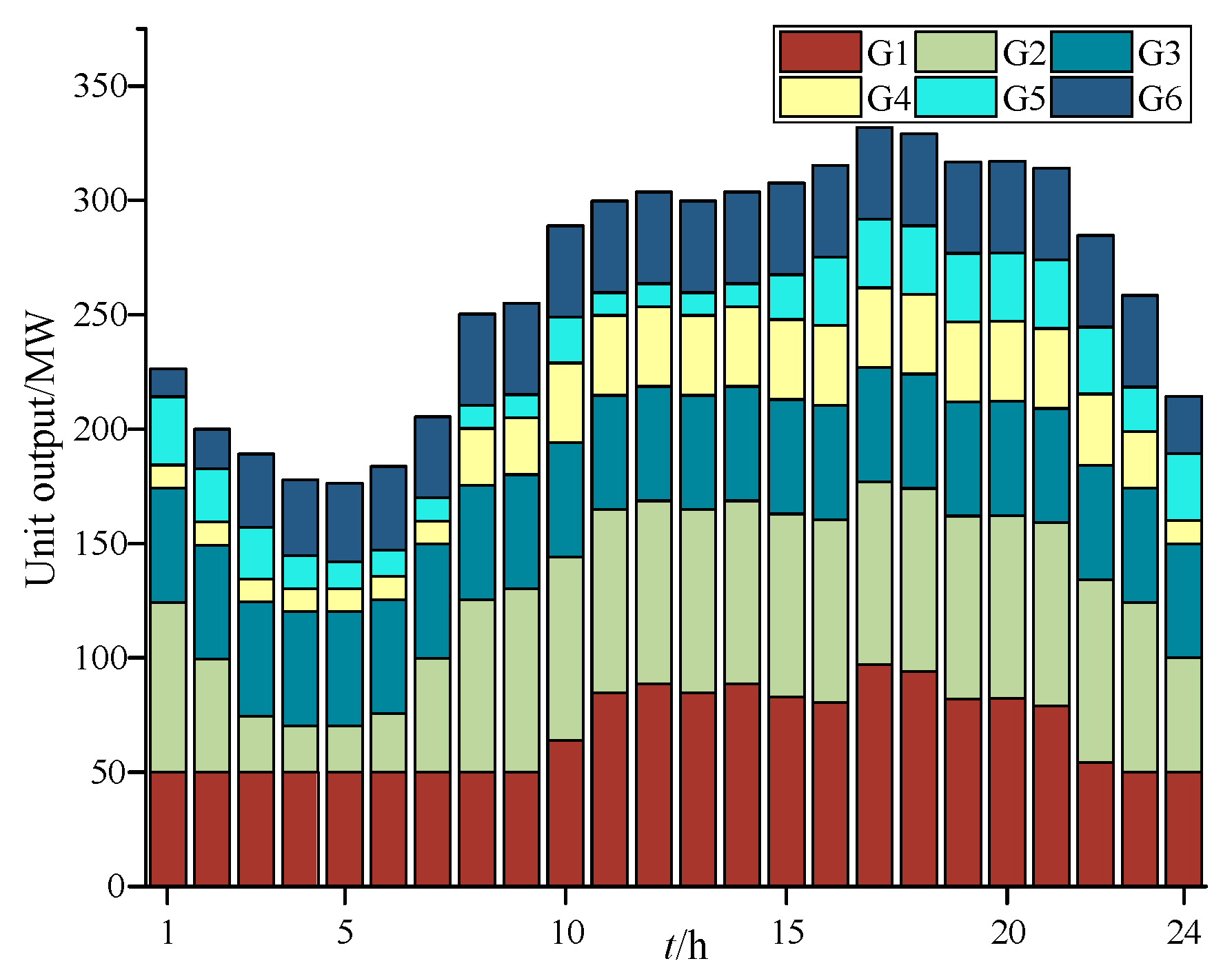
In addition, the day-ahead optimal scheduling results in this paper are shown in
Figure 4.
It can be seen from
Figure 4 that thermal power units G1, G2 and G3 bear the basic load of the system, and G3 is always in full load state during the dispatching period. In the period from t = 1 to t = 6, due to the reduction of load demand, the system adapts to reduce the output of G2 to balance the load constraint; while in the period from t = 6 to t = 12, the system constraint is satisfied by increasing the output of G2.
4.1.3. Comparative Analysis
In order to verify the correctness and effectiveness of the method proposed in this chapter, the following three scenarios are set up:
Scenario 1: Day-ahead optimal scheduling without considering carbon emissions trading;
Scenario 2: Considering the carbon emission trading of the power system, the carbon emission quota allocation method based on the weighted average of the electricity marginal emission factor and the capacity marginal emission factor is used;
Scenario 3: Considering the carbon emission trading of the power system, and using the carbon emission quota allocation method based on the entropy method; that is, the model in this paper.
- (1)
Considering the necessity of the verification of carbon emission trading
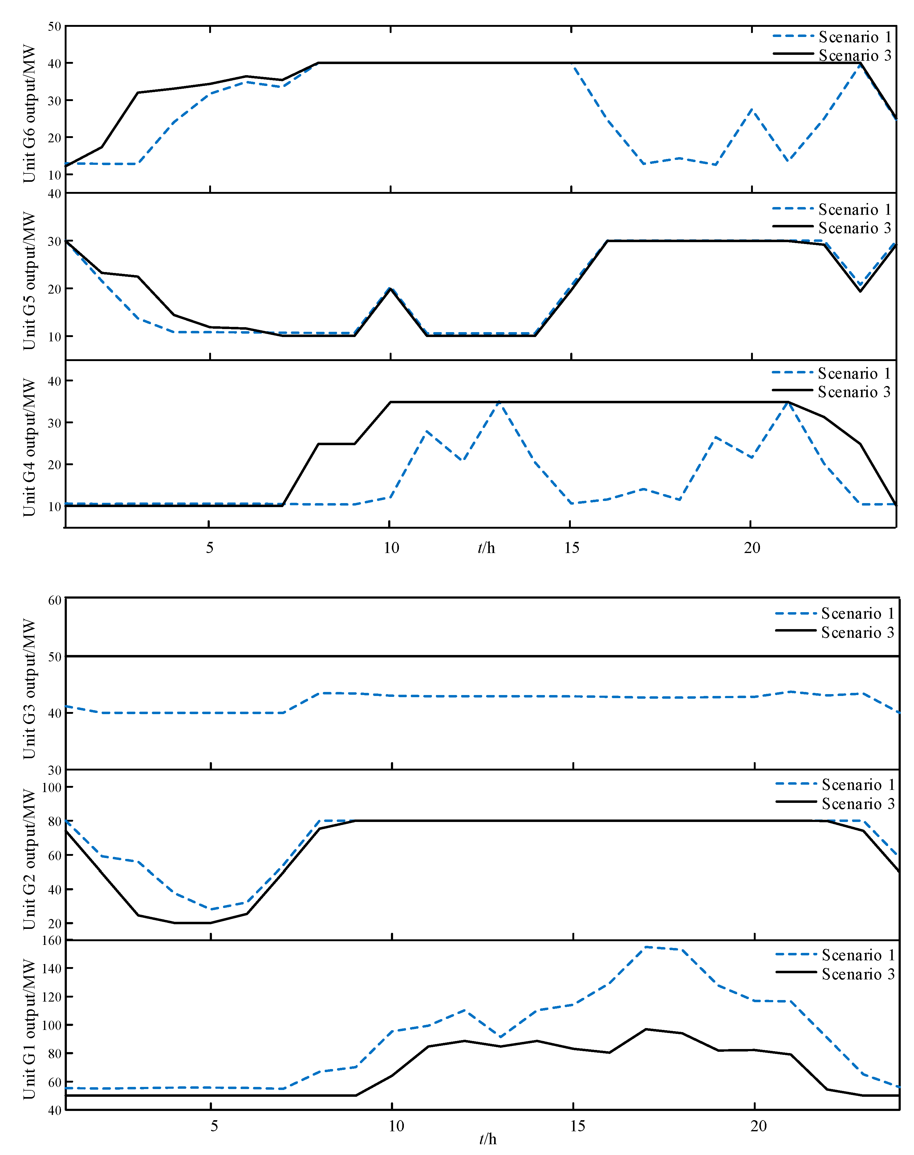
In order to verify the necessity of incorporating carbon trading into the day-ahead optimal scheduling model, the total carbon emissions of Scenario 1 and Scenario 3 are calculated and analyzed. Firstly, the output plan of each unit under Scenario 1 and Scenario 3 in the dispatching period is shown in
Figure 5.
It can be seen from
Figure 5 that compared with Scenario 1, the output level of units G1 and G2 bearing the basic load of the system in Scenario 3 is obviously reduced for the whole dispatching period, in which the output of G1 is reduced most obviously, while the output of units G3, G4, G5 and G6 is significantly increased. This is because the carbon emissions of thermal power units are positively correlated with the unit output. For units G1 and G2, with large active power output and high carbon emission levels, in order to reduce the system carbon emissions in each dispatching period, the Scenario 3 model reduces the output of G1 and G2. For units G3, G4, G5 and G6, with small output and low carbon emission levels, the corresponding active power output is increased. Therefore, incorporating carbon trading into the day-ahead optimal dispatching model is mainly to reduce carbon emissions in each dispatching period by reducing the output of units with higher carbon emission levels, while increasing the output of units with lower carbon emission levels to ensure power supply balance.
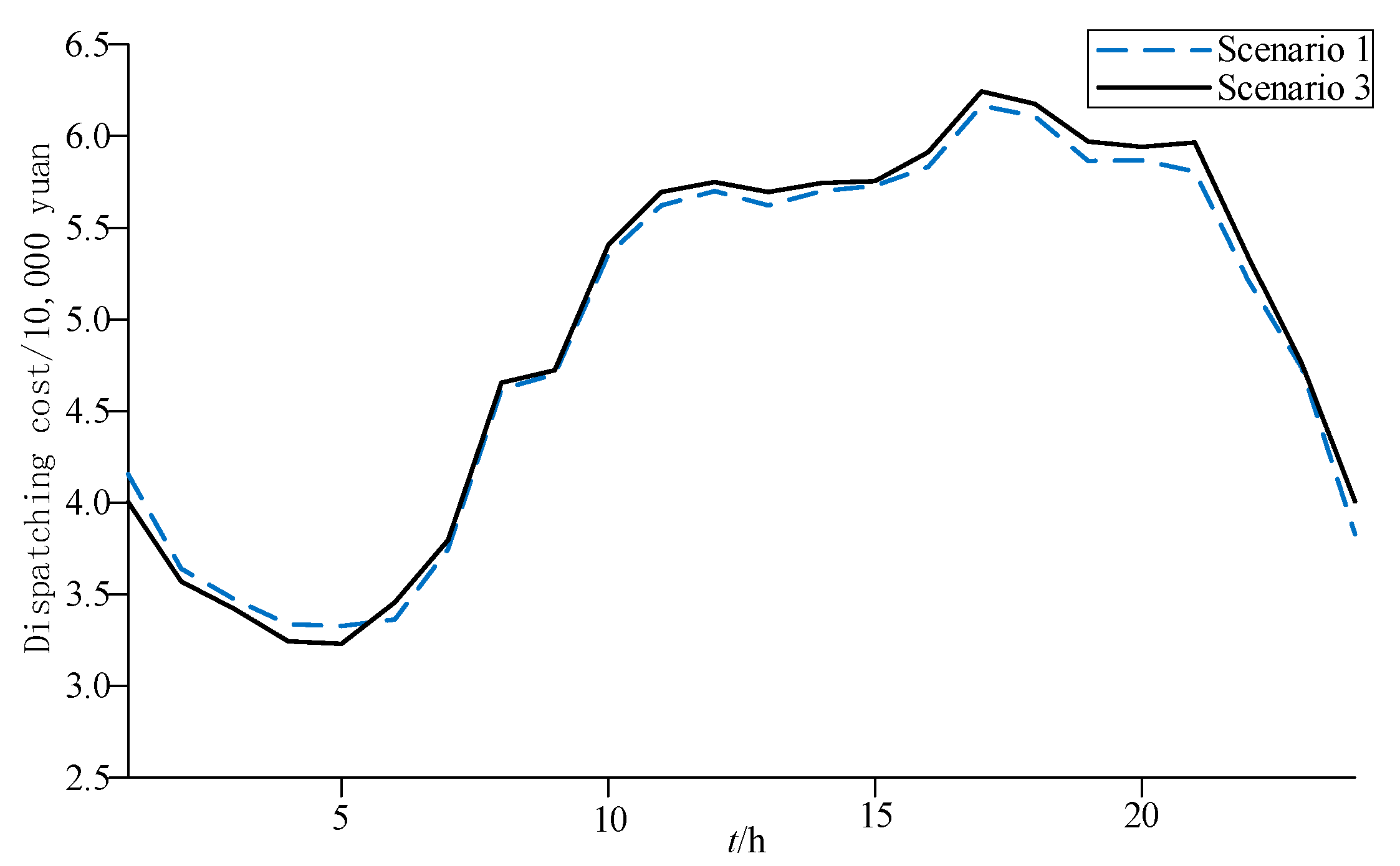
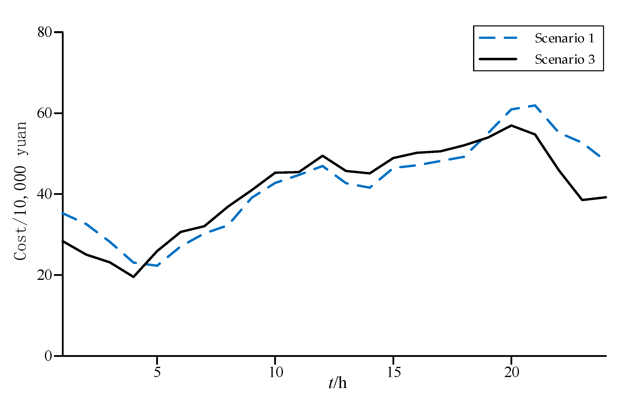
Furthermore, in order to analyze the change of the total cost of the system in the scheduling period after considering the carbon trading, the total cost of each period under the two scenarios is calculated, and the comparison chart is shown in
Figure 6.
It can be seen from
Figure 6 that in the period from t = 1 to t = 5, compared with Scenario 1, the system cost of Scenario 3 is reduced, mainly because the carbon trading income of wind power is greater than the carbon trading cost of thermal power units, thus offsetting part of the cost. In the period from t = 10 to t = 24, the dispatching cost of Scenario 3 is higher than that of Scenario 1, which is mainly due to the increase in output of G3, G4, G5 and G6 in the corresponding period, resulting in the carbon trading cost of thermal power exceeding the carbon trading income of wind power. For the whole dispatching period, the total cost of Scenario 3 is 18,700 yuan higher than that of Scenario 1. Combined with Scenario 3 in
Figure 5, although the output of G1 and G2 is reduced to limit carbon emissions, the total cost will eventually increase to a certain extent. Therefore, incorporating carbon emissions trading into the day-ahead scheduling model is essentially to reduce the total carbon emissions of the system by reducing the output of high-emission units while increasing the output of low-emission units at the cost of a small increase in the total cost.
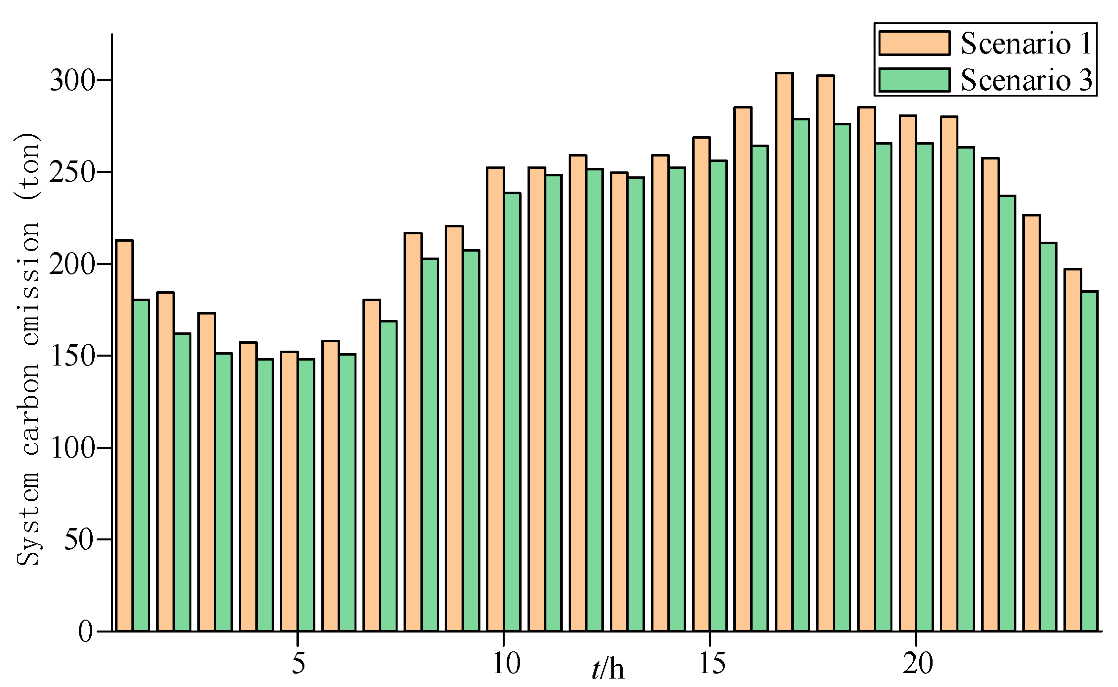
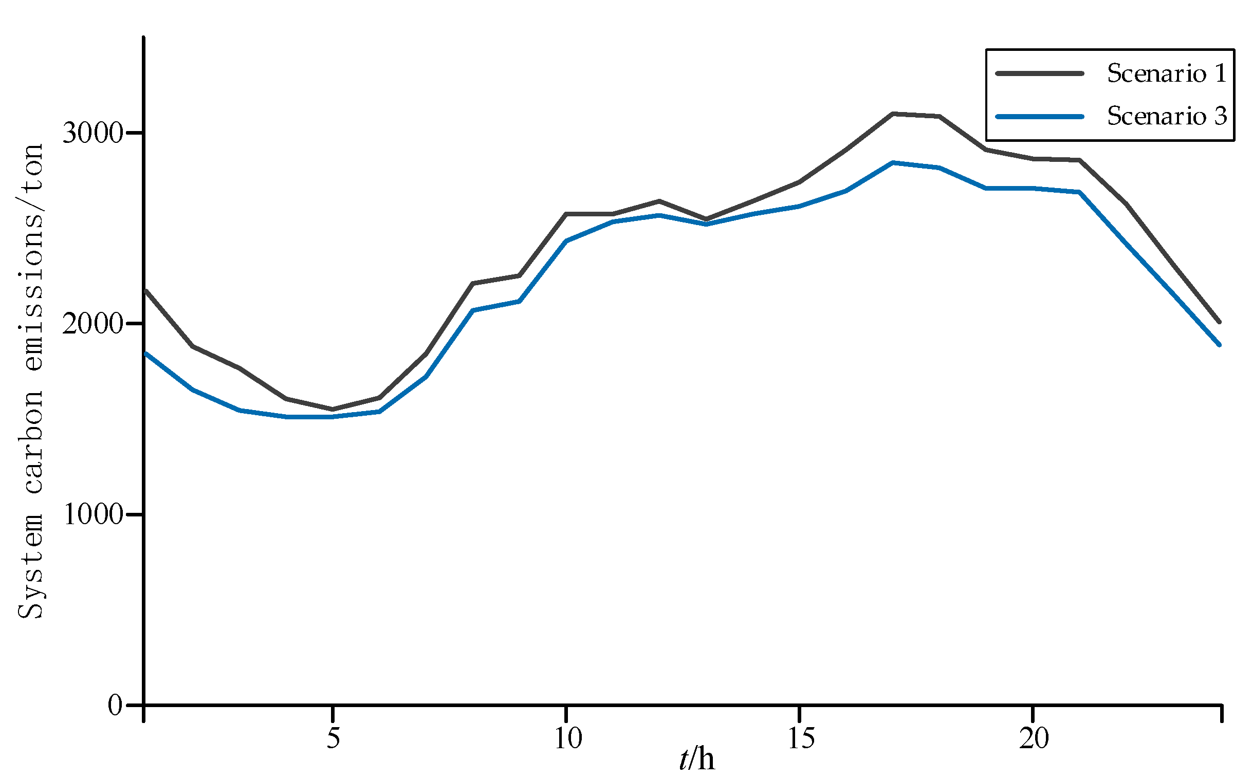
Then, the total carbon emissions of the system in each scheduling period under Scenario 1 and Scenario 3 are calculated, as shown in
Figure 7.
It can be seen from
Figure 7 that the carbon emissions of Scenario 3 are significantly lower than those of Scenario 1. In the whole scheduling period, the total carbon emission from the Scenario 1 system is 5616.36 tons, while the total carbon emission of Scenario 3 is 5262.33 tons, which reduces carbon emissions by nearly 354 tons compared with Scenario 1. Therefore, incorporating carbon emission trading into the day-ahead scheduling model can effectively reduce the total carbon emission of the system.
- (2)
Validity verification of the carbon emission quota allocation method based on the entropy method
The output results of each unit under Scenario 2 and Scenario 3 are shown in
Table A2 and
Table A3 of
Appendix A, respectively. In order to verify the effectiveness of the carbon emission quota allocation method based on the entropy method, the total carbon emission quota of each unit in Scenario 2 and Scenario 3 is calculated, and the specific results are shown in
Table 2.
It can be seen from
Table 2 that the carbon emission quota of G1 in Scenario 3 is higher than that in Scenario 2. By comparing the output results of G1 in the two scenarios, the carbon emission quota is actually reduced by lowering its output. Compared with Scenario 2, the output of G4 and G6 units with lower carbon emission intensity in Scenario 3 increases significantly, and their corresponding carbon emission quotas also increase accordingly. In addition, the carbon emission quota of thermal power units G2, G3 and G5 is higher than that of Scenario 2. This is because the method of calculating the carbon quota coefficient based on the entropy method takes into account the carbon emission characteristics of different units. Compared with the method of directly averaging carbon emission factors, the increase of the carbon quota coefficient leads to a corresponding increase of the carbon emission quota.
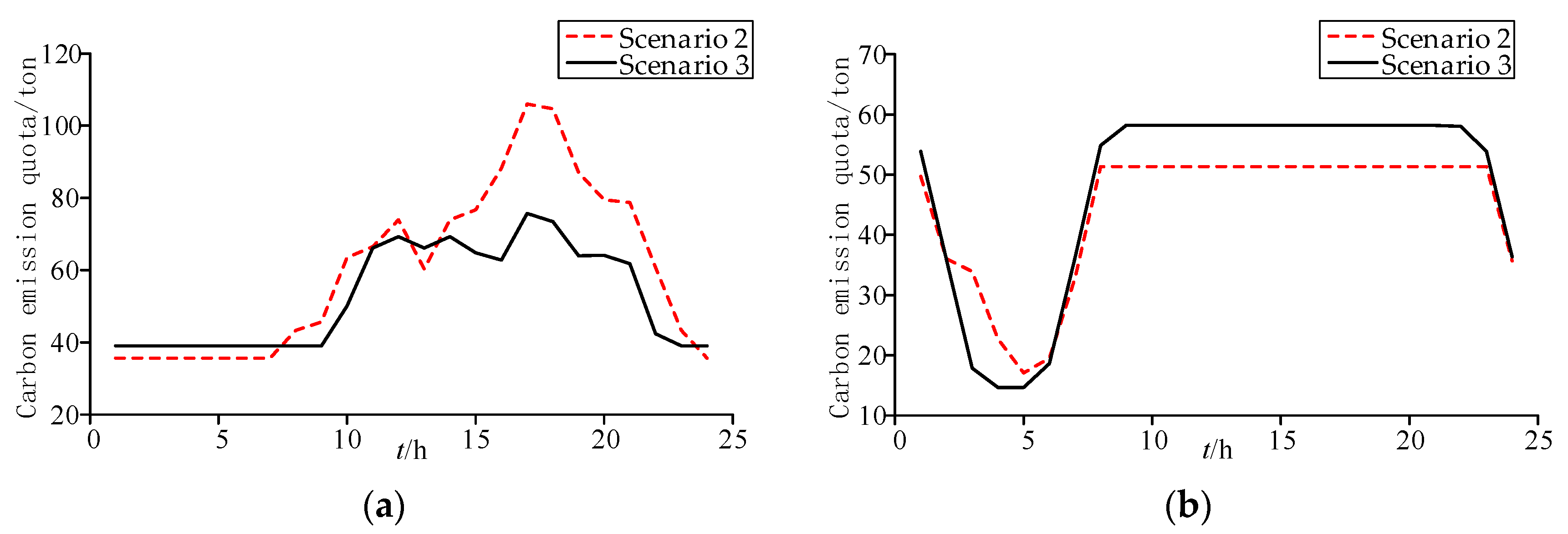
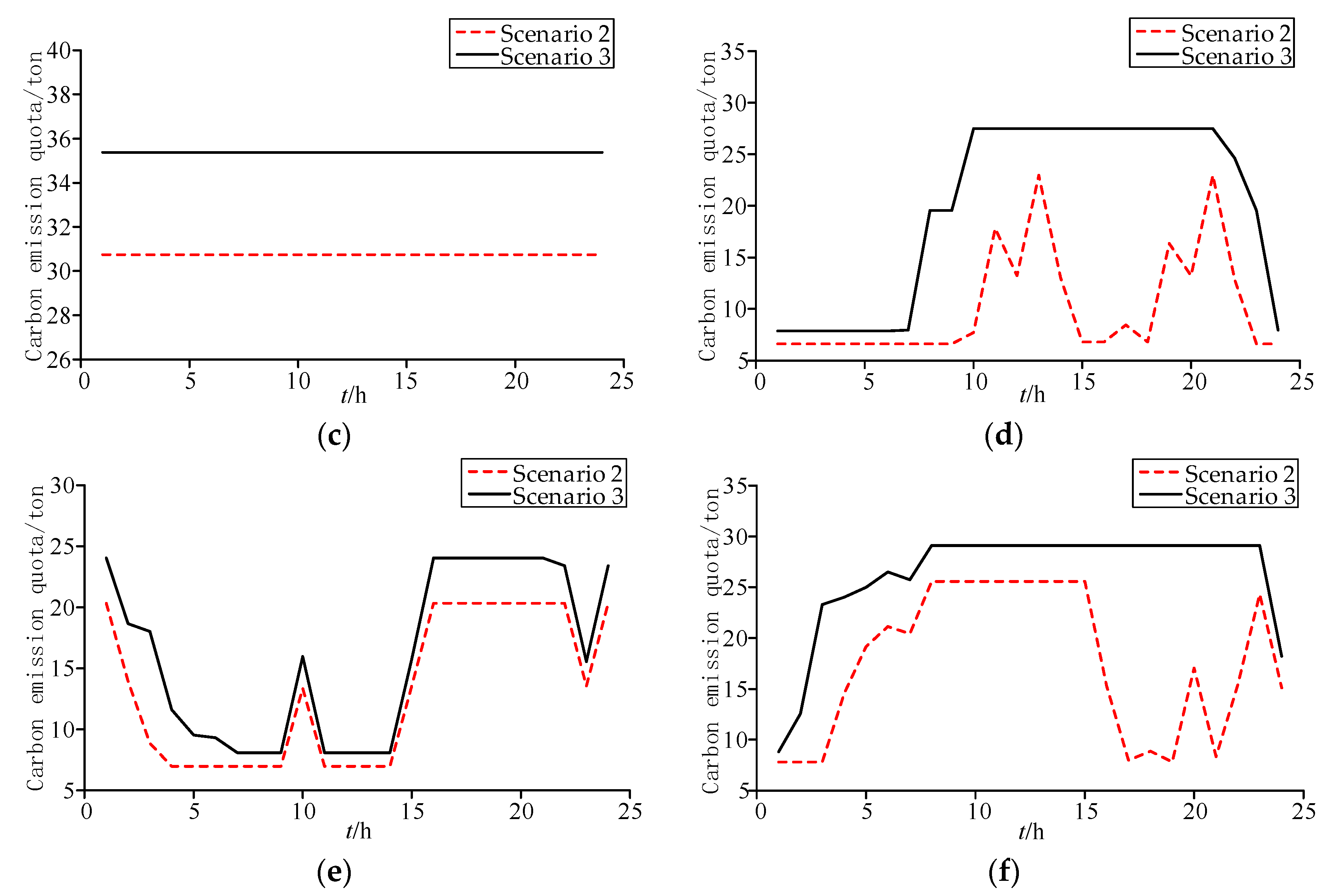
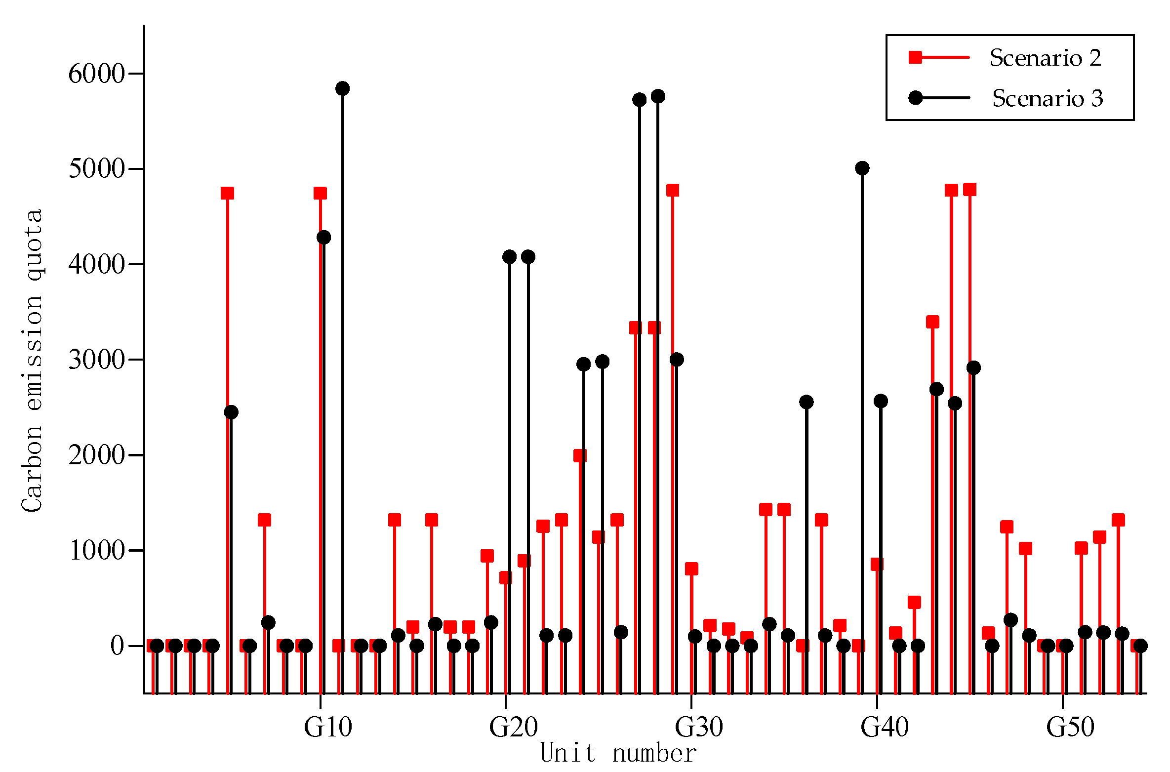
In addition, in order to analyze the impact of the carbon emission quota allocation method in this paper on different units, the carbon emission quotas of each unit in Scenario 2 and Scenario 3 are compared in detail. The carbon emission quotas of six thermal power units in the dispatching period are shown in
Figure 8.
It can be seen from
Figure 8 that for unit G1 bearing the base load, compared with Scenario 2, the carbon emission quota of Scenario 3 from t = 14 to t = 23 is significantly reduced. The main reason is that the output level of unit G1 is more stable, and the total active output is significantly reduced in Scenario 3. For unit G2, the carbon emission quota under Scenario 3 is significantly higher than that under Scenario 2 from t = 8 to t = 24, and the output levels of the two scenarios are basically the same. The main reason for the increase of the G2 quota is that the quota coefficient of Scenario 3 is higher than that of Scenario 2. For unit G3 with unchanged unit output under the two scenarios, the quota of Scenario 3 is higher than that of Scenario 2, which is also caused by the increase of the quota coefficient. For units G4, G5 and G6, their quotas under Scenario 3 are higher than those under Scenario 2. The common reason for the increase of their carbon emission quotas is that they are affected by the increase of the quota coefficient. In addition, the output of G4 and G6 increases significantly and remains within a certain range due to their undertaking the reserve required for wind power access. These two reasons make the quotas of G4 and G6 increase under Scenario 3. Therefore, this method not only optimizes the carbon emission quota of each unit, but also makes the output level of the unit more stable.


