Calibration and Evaluation of the WRF-Hydro Model in Simulating the Streamflow over the Arid Regions of Northwest China: A Case Study in Kaidu River Basin

Abstract

In this study, the hydrological system of the Weather Research and Forecasting model (WRF-Hydro) is applied to simulate the streamflow at the Kaidu River Basin, which is vital to the ecological system in the lower reaches of the Tarim River in Northwest China. The offline WRF-Hydro model is coupled with the Noah multi-parameterization land surface model (Noah-MP) and is forced by the China Meteorological Forcing Dataset (CMFD), with the grid spacing of the hydrological routing modules being 250 m. A 3-year period (1983–1985) is used for calibration and a 17-year period (1986–2002) for the evaluation. Several key parameters of WRF-Hydro and four Noah-MP parameterization options are calibrated, and the performance of WRF-Hydro with the optimized model setting is evaluated using the daily streamflow observations. The results indicate that WRF-Hydro can reproduce the observed streamflow reasonably, with underestimation of the streamflow peaks. The simulated streamflow is sensitive to the parameters of bexp, dksat, smcmax, REFKDT, slope, OVROUGHRTAC and mann in the Kaidu River Basin. At the same time, the parameterization options of Noah-MP also have a large influence on the streamflow simulation. The WRF-Hydro model with optimized model settings can achieve correlation coefficient (CC) and Nash efficiency coefficient (NSE) statistical scores of 0.78 and 0.61, respectively, for the calibration period. Meanwhile, for the evaluation period, the scores are 0.7 and 0.50, respectively. This study indicates the importance of applying the physical-based WRF-Hydro model over Northwest China and provides a reference for the nearby regions.

1. Introduction

The water resources in the arid regions of Northwest China are highly susceptible and vulnerable to the effects of both climate change and human activities [1,2,3]. In recent decades, the expansion of human populations and economic development in the arid regions have exacerbated the conflict between water supply and demand, resulting in rapid degradation in the quality of the ecological environment [4]. For instance, the groundwater table along the Tarim River has declined from 2–3 m to 4–10 m after the 1970s [5], and over 10,000 km² of land has been affected by desertification, particularly for the Populus euphratica forest along the river [6]. To ensure the security of the ecological system in the lower reaches of the Tarim River, a large ecological water conveyance project has been implemented by the local government, transferring water from the Kaidu River to the lower reaches of the Tarim River Basin for the past two decades [7], and observations have indicated that this ecological water conveyance has increased the groundwater table and has a significant influence on the restoration of vegetation in the lower reaches of the Tarim River [1]. As the project relies on water from the Kaidu River, accurate prediction and an in-depth understanding of streamflow variations of the Kaidu River are crucial for the local area [8,9].

In arid regions, the water, energy and ecological processes between the atmosphere, land surface and subsurface are strongly coupled, and numerous studies have emphasized the importance of integrated representation of terrestrial hydrological dynamics in the development of meteorological models [10,11,12], as most of the current weather and climate models oversimplify hydrological processes by using a one-dimensional (vertical) approach that neglects lateral water movement and the subsequent re-infiltration and exfiltration processes. This oversimplification can lead to errors in the representation of hydrologic conditions in models, especially for complex terrain and areas with moisture gradients. The Weather Research and Forecasting (WRF) model [13] is one of the most popular mesoscale models and shows good performance in simulating and predicting major meteorological variables such as temperature, precipitation and wind speed over China [14,15,16,17,18]. The hydrological enhancement system of the WRF model, named WRF-Hydro [19,20], is a fully distributed, multi-physical and multi-scale three-dimensional land surface hydrological simulation system that considers the lateral redistribution of surface, subsurface, groundwater and channel water. As a result, it can better describe the relationship between water and energy fluxes at the atmospheric–terrestrial interface. The WRF-Hydro model can be applied as an offline model for model calibration and flood simulation [21] and as a coupled model for studying the land–atmosphere feedback [22,23,24,25,26,27]. A growing number of studies have been conducted with WRF-Hydro over China, either in the uncoupled or coupled mode [22,24,25,26,27,28,29,30,31]. For example, Wang et al. [22] studied the spatiotemporal characteristics of rainfall and several key water cycle elements, including soil moisture, evapotranspiration and runoff over North China, the results show that the fully coupled WRF/WRF-Hydro system produced slightly less runoff but more frequent infiltration and higher soil moisture than the WRF-only simulations. Liu et al. [30] investigated the effects of four key parameters on the streamflow simulation over North China and found that the runoff infiltration parameter and the channel Manning roughness parameter are the most sensitive parameters, particularly under unsaturated soil conditions. Wang et al. [26] used WRF-Hydro to simulate the climate hydrological coupling situation of the Daihai Basin in North China from 1980 to 2020, and the simulations showed that the inflow of Daihai Lake decreased during the study period and that the runoff into the lake tended to be flat since 2013.

Although many simulations were conducted in different regions of China in previous studies, there are almost no applications of WRF-Hydro in the arid regions of Northwest China. For the Kaidu River Basin of Northwest China, accurate simulation of natural streamflow is of utmost importance for the local government. It can provide the necessary scientific support for effective reservoir operation and agricultural planning. Despite their significance, such simulations have yet to be carried out in this region. Thus, in this study, we apply version 5.1.2 of the WRF-Hydro model to simulate the streamflow of the Kaidu River, investigate the model’s sensitivity to the key parameters affecting its behavior and assess the performance of the WRF-Hydro model with the calibrated parameters. The results of this study could provide valuable references for further research in the study area and nearby regions.

2. Materials and Methods

2.1. Study Area

The Kaidu River Basin is located at the edge of the Taklimakan Desert, the second largest desert in the world. It originates from the southern slope of the Tianshan Mountains in northwestern China and flows into Bosten Lake, which is the headwater of the downstream Tarim River that ultimately flows into the Lob Nor. The basin’s bottom elevation ranges from approximately 2300 to 2600 m above sea level [8]. The climate in the basin is continental temperate arid, with a mean annual temperature of −4.2 °C in the mountainous area (Bayinbuluke station, as shown in Figure 1) for the period 1961–2010. The Kaidu River is the primary contributor to Bosten Lake, accounting for over 80% of the inflowing water, and the annual runoff at the Dashankou hydrological station (as illustrated in Figure 1) is 35.05 × 10⁸ m³ for the period 1961–2010, primarily originating from snow- and ice melt and rainfall. The accumulation of snow typically begins in November and ends in March of the following year, while mountain snowmelt and rainfall are the primary water sources of the river during the summer months [9].

2.2. WRF-Hydro Model Structure and Configuration

In this study, the WRF-Hydro model is used, the model extends the traditional one-dimensional land surface schemes in WRF by providing a framework for multiple terrestrial physics options, such as overland flow, subsurface flow, channel flow and a bucket model to account for baseflow. The model can be used as a hydrological model, which is referred to as the ‘one-way coupling’, ‘offline’ or ‘standalone’ mode, where the model applies a one-way process using gridded atmospheric forcing variables, including incoming shortwave and longwave radiation, specific humidity, air temperature, surface pressure and near-surface wind. Alternatively, the model can be run in a fully coupled mode with information exchange between the land surface model and the atmospheric model; in this case, the atmospheric model can provide the meteorological forcing, and no additional inputs are necessary for the land surface model. This configuration is often referred to as the ‘fully’ or ‘two-way coupling’ mode.

The default land surface model for WRF-Hydro 5.1.2 is the Noah-MP model [32,33], which is developed based on the Noah model [34] and features multiple parameterization options. In contrast to its predecessor, the Noah model, the Noah-MP model offers an expanded range of user-selectable process schemes, including canopy stomatal resistance scheme, dynamic vegetation scheme, snowpack parameterization and runoff/groundwater options. The default physics options of Noah-MP are listed in Table S1. The soil column in Noah-MP has a 2 m profile, subdivided into 4 layers with thicknesses of 10, 30, 60 and 100 cm, respectively.

In this study, the grid spacing of the Noah-MP model is 1 km, and the simulation domain covers the Kaidu River Basin and the surrounding areas, consisting of 300 grids in the west–east direction and 160 grids in the south–north direction. The subgrid routing modules of WRF-Hydro, on the other hand, have a horizontal grid spacing of 250 m, resulting in an aggregation factor of 4. As a result, the WRF-Hydro modules have 1200 grids in the west–east direction and 640 grids in the south–north direction, and the timestep of terrain routing and channel routing is 6 s. For each timestep, the soil conditions within the Noah-MP model are disaggregated from the land surface grids to the high-resolution routing grid through a subgrid, spatial weighting method [19]. The relevant input fields passed from Noah-MP to the routing modules include maximum soil moisture for each soil type, infiltration capacity excess, lateral saturated hydraulic conductivity for each soil type and soil moisture content for each soil layer.

The high-resolution routing fields were generated from elevation data extracted from the HydroSHEDS DEM (https://www.hydrosheds.org (accessed on 10 January 2022)). Channel parameters, such as stream order and flow direction, are presented in Figure S1 for the river basin. The land use dataset used in this study is the Moderate Resolution Imaging Spectroradiometer (MODIS) modified International Geosphere–Biosphere Program (IGBP) 20-category land cover product (Figure S1) developed by the Chinese Academy of Sciences (CAS) [15], and soil type information was obtained from the global soil dataset created by Beijing Normal University [35]. Based on the CAS land cover dataset, the basin was mainly classified into three land cover types: grasslands, open and closed shrublands and barren or sparsely vegetated areas. The land surface properties, including canopy height, maximum carboxylation rate and overland flow roughness, are dependent on land cover type, while the soil hydraulic parameters (i.e., soil porosity, grain size distribution index and saturated hydraulic conductivity) are based on the soil texture types. The physically based one-dimensional column snowpack model (Crocus) was activated during the simulation.

The China Meteorological Forcing Dataset (CMFD), a high-resolution gridded near-surface meteorological dataset over China [36], was utilized to provide meteorological forcing for WRF-Hydro. This dataset has a spatial resolution of 0.1° and 3-hourly temporal resolution and has been validated to be superior to the GLDAS (Global Land Data Assimilation System) when compared to observations. Surface overland, saturated subsurface and channel routing were activated for the routing module in the WRF-Hydro model. The steepest descent for the surface overland flow routing and diffusive wave for the channel routing were used.

Due to the limitation of computational resources, a three-year period (1983–1985) was selected as the calibration period, and for each calibration run, the model performance was evaluated using the simulation results and the daily streamflow observations of the Dashankou station (Figure 1). Then, the model was run for the period of 1986–2002 with the optimized model options, and the performance was evaluated with the observations.

2.3. Experimental Design

The WRF-Hydro model has several hydrological parameters that require adjustment or calibration based on the hydrological characters of the study region. In this study, we selected 12 parameters for calibration guided by prior studies [11,29,30,37]; details of the parameters are listed in

Table 1. List of the parameters tested in the sensitivity experiments.

Name	Description	Units	Default Value	Calibration Factor
bexp	Pore size distribution index		×1	multiple
expon	Bucket drainage parameter		3
dksat	Saturated hydraulic conductivity	m/s	×1	multiple
smcmax	Saturation soil moisture content	fraction	×1	multiple
REFKDT	Surface runoff parameter		3
slope	Openness of bottom drainage boundary		0.1
RETDEPRTFAC	Multiplier on retention depth limit		1
LKSATFAC	Multiplier on lateral hydraulic conductivity		1000
OVROUGHRTAC	Multiplier on Manning’s roughness		1
mann	Channel Manning roughness		×1	multiple
Zmax	Maximum groundwater bucket depth	mm	50
mfsno	Melt factor for snow depletion curve		2.5

.

Among the parameters, the soil saturated hydraulic conductivity (dksat) regulates the speed at which water moves through the subsurface and is commonly calibrated in combination with the pore size distribution index (bexp) parameter, and the latter parameter controls how actual conductivity is scaled from saturated conductivity based on soil water content. The slope parameter, initially estimated from the land surface topography, determines the openness or closure of the bottom boundary of the soil column. The REFKDT parameter controls how easily precipitation reaching the surface infiltrates into the soil column, with higher values of REFKDT leading to more infiltration and less surface runoff. The RETDEPRTFAC parameter is a multiplier on the maximum retention depth, whereas the LKSATFAC parameter is a multiplier on the prescribed lateral saturated hydraulic conductivity values. The overland flow roughness parameter is regulated by the OVROUGHRTFAC parameter, which, in turn, is determined by land use type and affects the speed of overland transmitters downstream. Finally, the Mann parameter reflects the influence of channel roughness on streamflow.

To calibrate the model, we utilized a stepwise approach outlined in [11], as automated calibration methods, such as the dynamically dimensioned search algorithm [38], would require a large number of simulations and considerable computational resources. In this study, we calibrated each parameter listed in Table 1 individually and retained its calibrated value for subsequent steps. Finally, we evaluated the model’s performance against observed streamflow data by running the model with the calibrated parameters.

2.4. Evaluation Metrics

The performance of the WRF-Hydro model is evaluated by four commonly used metrics: correlation coefficient (CC), model bias (BS), root mean squared error (RMSE) and Nash efficiency coefficient (NSE). The CC reflects the linear relationship between simulations and observations. The NSE is a commonly used metric in hydrological evaluations as it takes into account both the magnitude of errors and the variability of timeseries. The RMSE is used to quantify the deviation between the simulations and observations. They are defined as follows:

$$CC=\frac{{\sum }_{i=1}^N\left(M_i-\overline{M}\right)\left(O_i-\overline{O}\right)}{\sqrt{{\sum }_{i=1}^N{\left(M_i-\overline{M}\right)}^2·{\sum }_{i=1}^N{\left(O_i-\overline{O}\right)}^2}}$$

$$BS=100\%\times \frac{{\sum }_{i=1}^N\left(M_i-O_i\right)}{{\sum }_{i=1}^N{O}_i}$$

$$RMSE=\sqrt{\frac{1}{N}{\sum }_{i=1}^N{\left(M_i-O_i\right)}^2}$$

$$NSE=1-\frac{{\sum }_{i=1}^N{\left(O_i-M_i\right)}^2}{{\sum }_{i=1}^N{\left(O_i-\overline{O}\right)}^2}$$

Here, $m_i$ is the value of the model simulation, $o_i$ is the value of the observation, N is the number of observations and $\overline{O}$ and $\overline{M}$ are the average of observation and model simulations, respectively.

3. Results

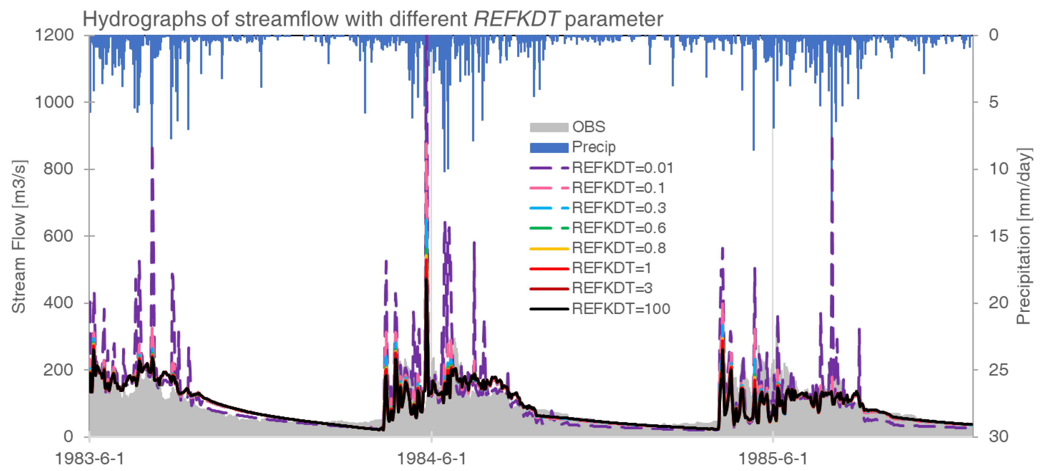
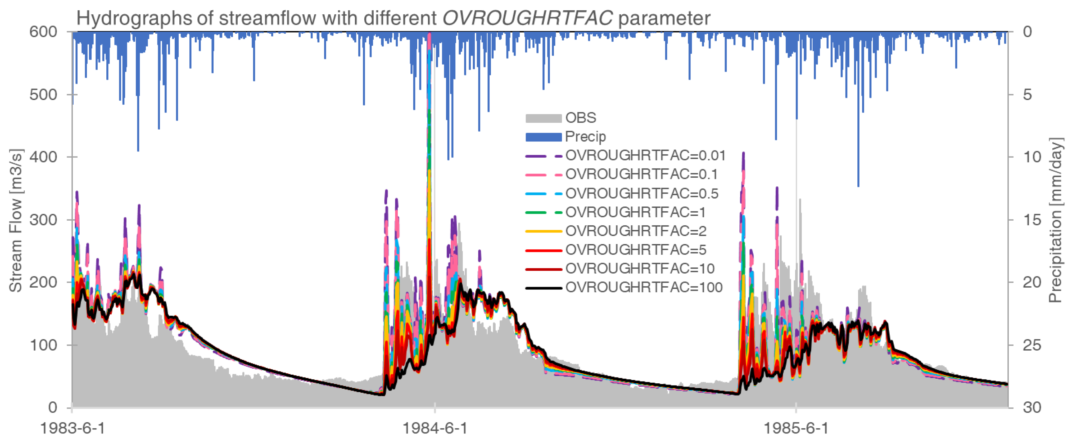
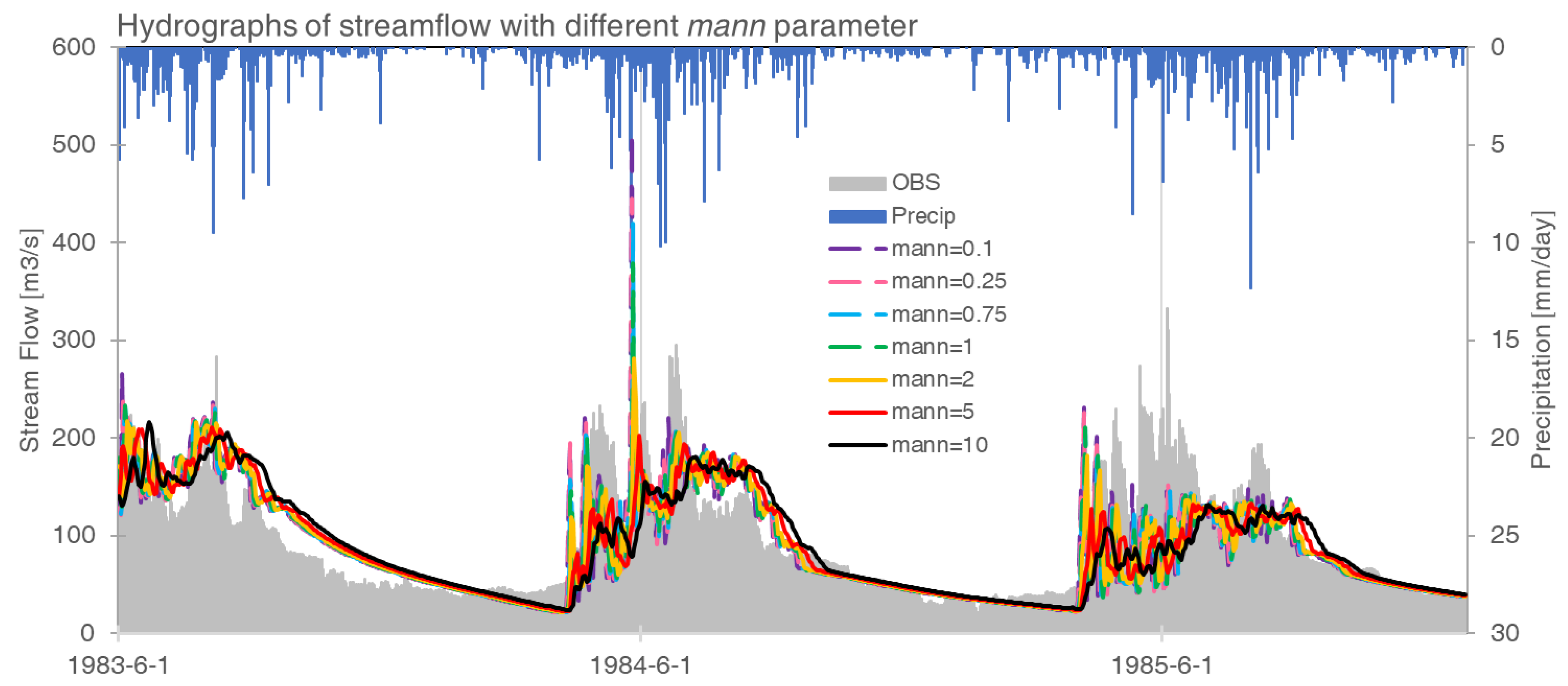
3.1. Model Sensitivity to Key Parameters

Figure 2 shows the results of calibrating the bexp parameter by running the model with a range of values from 0.1 to 10. During the calibration period of 1983–1985, the peak discharge occurs approximately between June and August, while baseflows are generally reached by October. The figure demonstrates that bexp has a significant impact on streamflow simulation, where higher bexp values lead to lower streamflow. In the WRF-Hydro model, bexp controls how actual conductivity is scaled from saturated conductivity based on soil water content, and higher bexp values encourage more water to infiltrate into the soil column, thereby reducing surface runoff, which delays and decreases the runoff peaks. For example, the model run with a bexp value of 0.1 indicates runoff peaks exceeding 2000 m³/s, while the model run with a bexp value of 1 indicates peaks of less than 500 m³/s.

For the statistical scores, the CCs range from 0.71 to 0.73, the BCs range from −71.75 to 75.13%, the RMSEs range from 43.39 to 566.79 m³/s and the NSEs range from 0.50 to 0.60 for all the simulations with different bexp values. Based on these scores, a lower bexp value of 0.4 is considered an optimum value, with CC, BC, RMSE and NSE values of 0.71, 4.19 m³/s, 45.19% and 0.51, respectively. Similar diagrams for selecting the optimum value of the expon parameter with values ranging from 0.01 to 100 are shown in Figure S2. The simulated streamflow is not sensitive to expon, and there are few differences among simulations with different expon values. According to the statistical scores, a value of 10 for expon is chosen as optimal, with a CC of 0.72, BC of 4.53%, RMSE of 43.01 m³/s and NSE of 0.51.

Figure 3 depicts the calibration results of the dksat parameter with a range of values from 0.01 to 100. In the WRF-Hydro model, dksat represents the saturated hydraulic conductivity, which regulates the speed at which water moves through the subsurface. Although initial values of dksat are based on soil texture, reported ranges exhibit considerable variability. In general, higher values of dksat encourage faster soil water movement, which consequently reduces runoff peaks. Statistical evaluation of the sensitivity runs yielded CCs of 0.59–0.72, BCs of −43.06–4.41%, RMSEs of 43.01–94.51 m³/s and NSEs of 0.35–0.51. Based on these metrics, the default value of dksat (×1) is considered an optimum value.

Figure 4 illustrates the results for smcmax parameter with values ranging from 0.1 to 100. In the WRF-Hydro model, smcmax represents the maximum soil moisture content for each soil type, which has a large influence on flood generation. Generally, lower values encourage flash floods. In this study, the simulated streamflow is sensitive to smcmax, and the model spreads are large. The simulation with a value of 0.1 shows significant overestimation on the runoff peaks, both in amounts and values. In contrast, the simulation with a value of 100 underestimates the streamflow during the calibration period. The statistical scores of CC, BC, RMSE and NSE for all the experimental simulations are 0.68–0.80, −43.28–66.34%, 43.01–114.66 m³/s and 0.47–0.64, respectively. According to the statistical scores, the default value (×1) is chosen as optimal, yielding CC, BC, RMSE and NSE of 0.72, 4.53%, 43.01 m³/s and 0.51, respectively.

The hydrographs obtained from the sensitivity simulations with REFKDT ranging from 0.1 to 100 are shown in Figure 5. REFKDT is an important Noah-MP parameter that controls how easily precipitation reaching the surface infiltrates into the soil column versus stays on the surface where it can become surface runoff. It can be observed from the hydrographs in Figure 5 that lower values of REFKDT lead to less infiltration and more surface runoff. For example, the simulation with lower REFKDT (0.01) indicates extremely high runoff peaks of 1200 m³/s in 1984, while higher REFKDT substantially decreases the runoff peak values. The statistical scores of CC, BC, RMSE and NSE for all the sensitivity runs are 0.56–0.72, 1.56–4.57%, 42.93–96.04 m³/s and 0.31–0.51, respectively. Based on these metrics, the default value of REFKDT (3) is chosen as optimal. The hydrographs for selecting the optimum values of RETDEPRTFAC and LKSATFAC parameters are illustrated in Figures S3 and S4. RETDEPRTFAC is a multiplier on the maximum retention depth, and LKSATFAC is a multiplier on the prescribed lateral saturated hydraulic conductivity. However, the simulated streamflow is not sensitive to the values of RETDEPRTFAC and LKSATFAC in this study.

Figure 6 illustrates diagrams for selecting the optimal value of the OVROUGHRT parameter with a range of 0.01 to 100. In WRF-Hydro, OVROUGHRT is determined by land use type and affects the downstream overland transmitter speed, with a default value of 1.0. Lower values of OVROUGHRT lead to higher runoff peaks; for instance, the simulated runoff peak is over 600 m³/s in the sensitivity run with a value of 0.01, while in the simulation with a value of 100, the runoff peak is about 300 m³/s. The CCs range from 0.67 to 0.72, the BCs range from −1.91–7.08%, the RMSE range from 42.13 to 53.83 m³/s and the NSEs range from 0.45 to 0.52 for all the sensitivity runs. Based on these metrics, an OVROUGHRTFAC value of 2 is chosen as optimal, resulting in CC, BC, RMSE and NSE values of 0.72, 5.75%, 42.13 m³/s and 0.52, respectively.

The slope parameter controls how open or closed the bottom boundary of the soil column is. Lower values of slope retain more water in the soil column, resulting in higher runoff peaks. On the other hand, higher values allow more water to drain to the channel or to deeper baseflow, leading to higher baseflow (Figure S5). The default value of slope (0.1) is chosen as optimal based on the statistical scores.

Figure 7 displays the hydrographs of sensitivity tests conducted for the mann parameter. The mann parameter is adjusted by multiplying the initial values in WRF-Hydro codes by the calibration factor, which is constrained between 0.1 and 10. This means that the channel Manning roughness parameters themselves are not adjusted. For instance, if mann has a value of 2, the initial value of channel Manning roughness is multiplied by 2 for all channels to compute the new parameters. As a result, the spatial patterns of the parameters are preserved. Figure 7 illustrates that the mann parameter has a significant influence on the runoff peaks, and lower values of mann resulted in higher runoff peaks. The statistical scores of CC, BC, RMSE and NSE for all the sensitivity runs range from 0.69 to 0.73, 5.03% to 6.15%, 41.20 to 45.55 m³/s and 0.48 to 0.53, respectively. Based on the statistical scores, a multiplier of 2 is chosen as the optimum value, yielding CC, BC, RMSE and NSE values of 0.73, 5.55%, 41.20 m³/s and 0.53, respectively. The simulated streamflow is found to be insensitive to Zmax and mfsno parameters (Figures S6 and S7), and the differences among simulations with different values are negligible. Based on the statistical scores, the lower values of mfsno (2.5) and Zmax (10) are chosen as the optimum values, and the statistical scores of CC, BC, RMSE and NSE are 0.73, 5.57%, 41.12 m³/s and 0.54, respectively.

3.2. Sensitivity to Noah-MP Options

As the WRF-Hydro model is composed of the Noah-MP model, which describes the lateral routing of surface and subsurface water, as well as groundwater storage, the performance of Noah-MP plays a crucial role in streamflow simulations within the WRF-Hydro model [39]. In this study, the impact of Noah-MP options on the streamflow simulations is also investigated. Four physical parameterization options are tested, including the options for runoff, partitioning precipitation into rainfall and snowfall, glacier and surface resistance parameterizations (

Table 2. List of Noah-MP physical parameterizations tested in this study.

Physical Parameterizations	Option	Description
Runoff options (run)
	1	TOPMODEL with groundwater
	2	TOPMODEL with an equilibrium water table
	3	original surface and subsurface runoff
	4	BATS surface and subsurface runoff
Partitioning precipitation into rainfall and snowfall options (pcp)
	1	Jordan
	2	BATS: when SFCTMP < TFRZ + 2.2
	3	SFCTMP < TFRZ
Glacier options (gla)
	1	include phase change of ice
	2	ice treatment more like original Noah
Surface resistance option (res)
	1	Sakaguchi and Zeng [40]
	2	Sellers
	3	Adjusted Sellers to decrease RSURF for wet soil
	4	Option 1 for non-snow; rsurf = rsurf_snow for snow

).

The statistical scores of the sensitivity tests of Noah-MP options are presented in Table S2. Across all simulations, the CCs range from 0.38 to 0.78, the BCs range from −29.92% to 53.88%, the RMSEs range from 40.11 to 69.79 m³/s and the NSEs range from 0.14 to 0.61. Based on the statistical scores, the simulation of run3_pcp2_gla1_res3 (option 3 for runoff, option 2 for partitioning precipitation into rainfall and snowfall, option 1 for glacier and option 3 for surface resistance) is considered optimal, with a CC, BC, RMSE and NSE of 0.78, 41.79%, 54.16 m³/s and 0.61, respectively.

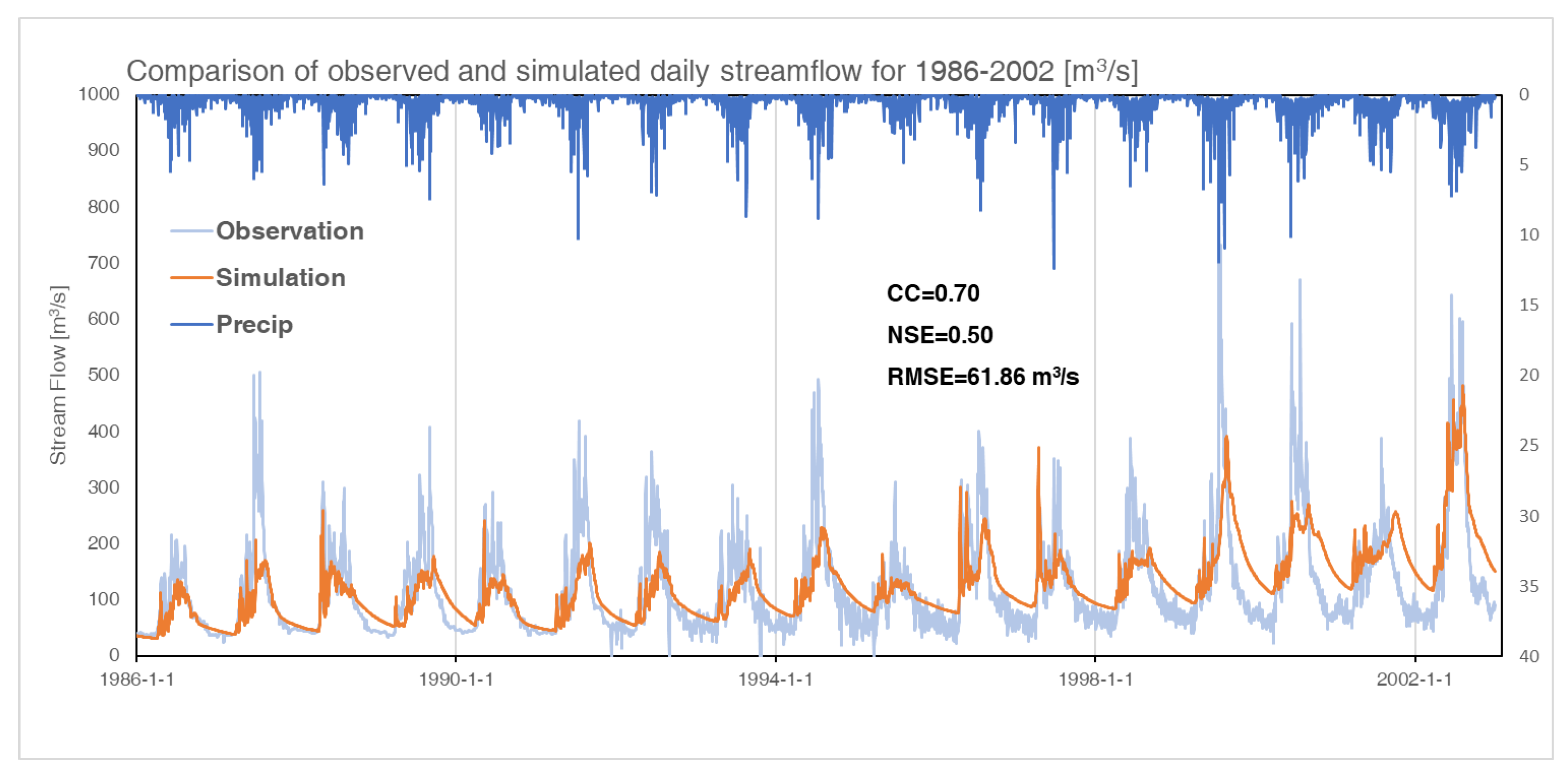
3.3. Model Performance Evaluation

To evaluate the model performance and examine the robustness of the model parameters, the optimized parameter set was applied in the evaluation period of 1986–2002. The simulated and observed daily streamflow time series and associated performance metrics are presented in Figure 8, where streamflow shows significant interannual variation with the peak flows ranging from about 200 m³/s in 1986 to about 800 m³/s in 1999. The WRF-Hydro model reproduces the streamflow trend, as well as dry and wet periods. The timing of simulated peak flows agrees with the observed ones, despite underestimation of peak flow magnitude, especially for wet years with peak streamflow exceeding 400 m³/s. However, the simulated baseflows show overestimation after 1996. Overall, the simulated daily flows agree with the observation, with CC and NSE values of 0.70 and 0.50, respectively.

The hydrographs of observed and simulated monthly streamflow for the evaluation period are shown in Figure S8, the hydrographs are smoother compared to the daily ones in Figure 8 and the WRF-Hydro model shows better performance in reproducing the streamflow on a monthly time scale. During the first ten years of the evaluation period, the model generally underestimates runoff peaks, especially for the wetter years of 1987, 1991, 1992 and 1994. For the years after 1996, WRF-Hydro reproduces the runoff peaks well; for example, for the years 1999 and 2002, the simulated peaks are very close to the observed ones. However, the model shows a significant overestimation of baseflow during the last ten years of the evaluation period. The statistical scores are higher than those for the daily time scale, with CC and NSE values of 0.76 and 0.58, respectively. According to previous studies [41,42], monthly streamflow model simulations are considered ‘good’ when NSE is greater than 0.65 and ‘satisfactory’ when NSE is greater than 0.50. Based on these metrics, the model performance in the Kaidu River Basin is found to be ‘satisfactory’.

4. Discussion and Conclusions

In this study, we calibrate and evaluate the physically based distributed WRF-Hydro modeling system in the Kaidu River Basin of Northwest China, with a grid spacing of 250 m. We investigate the sensitivity of simulated streamflow to twelve key parameters, including the pore size distribution index (bexp), bucket drainage parameter (expon), saturated hydraulic conductivity (dksat), saturation soil moisture content (smcmax), surface runoff parameter (REFKDT), openness of bottom drainage boundary (slope), multiplier on retention depth limit (RETDEPRTFAC), multiplier on lateral hydraulic conductivity (LKSATFAC), multiplier on Manning’s roughness (OVROUGHRTAC), channel Manning roughness (mann), maximum groundwater bucket depth (Zmax) and melt factor for snow depletion curve (mfsno). Additionally, we investigate four Noah-MP parameterizations (runoff, partitioning precipitation into rainfall and snowfall, glacier and surface resistance options) during the calibration period of 1983–1985. The model is manually calibrated using the stepwise calibration approach, and the optimized model setting is evaluated for the period of 1986–2002 using the correlation coefficient (CC), model bias (BS), root mean squared error (RMSE) and Nash efficiency coefficient (NSE) against observed daily and monthly streamflow.

The results indicate that the simulated streamflow is highly sensitive to variations in bexp, dksat, smcmax, REFKDT, slope, OVROUGHRTAC and mann, while the remaining five parameters exert minimal influence on the simulation. Furthermore, the selection of options in Noah-MP has a substantial impact on streamflow simulation, with appropriate choices leading to a 0.5 increase in the statistical scores of CC and a 1.1 increase in NSE. Importantly, the optimal parameter values identified in this study differ from those found in prior research conducted in other Chinese basins [29,30]. These discrepancies highlight the unique hydrological characteristics of arid regions and underscore the importance of model calibration prior to utilizing them for real streamflow simulations.

Our study demonstrates that the WRF-Hydro model, when optimized, reproduces the temporal distribution of daily runoff in the Kaidu River Basin during 1986–2002 reasonably. The model also captures the timing of runoff peaks. Our statistical analysis indicates only a slight decrease in performance compared to the calibration period, with daily CC, NSE and RMSE values of 0.70, 0.50 and 61.86 m³/s, respectively, and monthly CC, NSE and RMSE values of 0.76, 0.58 and 50.27 m³/s, respectively. These results highlight the model’s efficacy in simulating the hydrological characteristics of the Kaidu River Basin and its potential for use in future studies.

According to the evaluation metrics, the performance of WRF-Hydro in the Kaidu River Basin is classified to be ‘not good’, but ‘satisfactory’. However, streamflow simulation in arid regions presents significant challenges, as demonstrated by a similar study conducted in the Heihe River Basin in Northwest China, which also achieved an NSE of approximately 0.5 [24]. Nonetheless, such investigations are of great significance as they can provide a useful reference for nearby regions, given that the calibrated parameters can be successfully transferred to ungauged neighboring basins with similar physiography [11]. This is especially relevant for Northwest China where the availability of observations is limited.

The primary goal of this study is to conduct pioneering research on physically based streamflow simulations in the Kaidu River Basin. Given the strong human impacts in the basin in recent years, we selected an earlier time period (1983–1985) as the calibration period to better capture natural runoff processes and provide a scientific reference for water resource management in the region. Although some uncertainties may be introduced in this approach, such as the exclusion of some large flows in 1999 and 2000 from the calibration period, a physically based simulation of natural runoff is essential for local water resource management applications. In this study, biases in streamflow simulation may be linked to errors in precipitation. Over Northwest China, meteorological stations are sparse and mainly located in valley bottoms, introducing uncertainties in the forcing precipitation dataset of CMFD [29]. This is particularly important for peak flows, where model calibration already indicates some underestimation, and the potential missing of extreme precipitation at the local scale may also contribute to significant streamflow errors [39]. Liu et al. also reported the close relationship between the uncertainties of streamflow and driving precipitation [30], highlighting the importance of developing better precipitation forcing data for hydrological models.

Similar reductions in performance during the evaluation period have been observed in other studies [11,29,30,39,43], indicating the need for more in-depth calibrations in future work, which may involve the development of a new soil dataset for the arid regions of Northwest China with higher quality and resolution, as well as assignment of dynamic and distributed values to the newly developed soil dataset. To improve model performance, variable soil depths across the simulation domain will be investigated in future model versions.

References

1. Chen, Y.; Li, Z.; Fan, Y.; Wang, H.; Deng, H. Progress and prospects of climate change impacts on hydrology in the arid region of northwest China. Environ. Res. 2015, 139, 11–19. [Google Scholar] [CrossRef]
2. Xia, J.; Ning, L.; Wang, Q.; Chen, J.; Wan, L.; Hong, S. Vulnerability of and risk to water resources in arid and semi-arid regions of West China under a scenario of climate change. Clim. Change 2017, 144, 549–563. [Google Scholar] [CrossRef]
3. Tao, H.; Gemmer, M.; Bai, Y.; Su, B.; Mao, W. Trends of streamflow in the Tarim River Basin during the past 50years: Human impact or climate change? J. Hydrol. 2011, 400, 1–9. [Google Scholar] [CrossRef]
4. Xue, L.; Wang, J.; Zhang, L.; Wei, G.; Zhu, B. Spatiotemporal analysis of ecological vulnerability and management in the Tarim River Basin, China. Sci. Total Environ. 2019, 649, 876–888. [Google Scholar] [CrossRef]
5. Yan, H.; Wang, Y.; Wang, Y. The influence of 10 years of water conveyances on groundwater and juvenile Populus euphratica of the lower Tarim River. Env. Earth Sci. 2014, 71, 4091–4096. [Google Scholar] [CrossRef]
6. Chen, Y.; Chen, Y.; Xu, C.; Ye, Z.; Li, Z.; Zhu, C.; Ma, X. Effects of ecological water conveyance on groundwater dynamics and riparian vegetation in the lower reaches of Tarim River, China. Hydrol. Process. 2010, 24, 170–177. [Google Scholar] [CrossRef]
7. Wu, J.; Tang, D. The influence of water conveyances on restoration of vegetation to the lower reaches of Tarim River. Env. Earth Sci. 2010, 59, 967–975. [Google Scholar] [CrossRef]
8. Zhao, B.; Sun, H.; Yan, D.; Wei, G.; Tuo, Y.; Zhang, W. Quantifying changes and drivers of runoff in the Kaidu River Basin associated with plausible climate scenarios. J. Hydrol. Reg. Stud. 2021, 38, 100968. [Google Scholar] [CrossRef]
9. Xu, C.; Zhao, J.; Deng, H.; Fang, G.; Tan, J.; He, D.; Chen, Y.; Chen, Y.; Fu, A. Scenario-based runoff prediction for the Kaidu River basin of the Tianshan Mountains, Northwest China. Env. Earth Sci. 2016, 75, 1126. [Google Scholar] [CrossRef]
10. Balsamo, G.; Pappenberger, F.; Dutra, E.; Viterbo, P.; van den Hurk, B. A revised land hydrology in the ECMWF model: A step towards daily water flux prediction in a fully-closed water cycle. Hydrol. Process. 2011, 25, 1046–1054. [Google Scholar] [CrossRef]
11. Yucel, I.; Onen, A.; Yilmaz, K.K.; Gochis, D.J. Calibration and evaluation of a flood forecasting system: Utility of numerical weather prediction model, data assimilation and satellite-based rainfall. J. Hydrol. 2015, 523, 49–66. [Google Scholar] [CrossRef] [Green Version]
12. Senatore, A.; Mendicino, G.; Gochis, D.J.; Yu, W.; Yates, D.N.; Kunstmann, H. Fully coupled atmosphere-hydrology simulations for the central Mediterranean: Impact of enhanced hydrological parameterization for short and long time scales. J. Adv. Model. Earth Syst. 2015, 7, 1693–1715. [Google Scholar] [CrossRef]
13. Skamarock, C.; Klemp, B.; Dudhia, J.; Gill, O.; Liu, Z.; Berner, J.; Wang, W.; Powers, G.; Duda, G.; Barker, D.M.; et al. A Description of the Advanced Research WRF Model Version 4.1. In NCAR Technical Note; National Center for Atmospheric Research: Boulder, CO, USA, 2019. [Google Scholar]
14. Yu, E. A Warmer, wetter and less windy China in the twenty-first century as projected by a nested high-resolution simulation using the Weather Research and Forecasting (WRF) model. Asia-Pac. J. Atmos. Sci. 2019, 55, 53–74. [Google Scholar]
15. Yu, E.; Ma, J.; Sun, J. Developing a climate prediction system over Southwest China using the 8-km Weather Research and Forecasting (WRF) model: System design, model calibration and performance evaluation. Weather Forecast 2022, 37, 1703–1719. [Google Scholar] [CrossRef]
16. Yu, L.; Liu, Y.; Liu, T.; Yu, E.; Bu, K.; Jia, Q.; Shen, L.; Zheng, X.; Zhang, S. Coupling localized Noah-MP-Crop model with the WRF model improved dynamic crop growth simulation across Northeast China. Comput. Electron. Agric. 2022, 201, 107323. [Google Scholar] [CrossRef]
17. Gao, S. Dynamical downscaling of surface air temperature and precipitation using RegCM4 and WRF over China. Clim. Dyn. 2020, 55, 1283–1302. [Google Scholar] [CrossRef]
18. Gao, Y.; Xu, J.; Zhang, M.; Liu, Z.; Dan, J. Regional climate dynamical downscaling over the Tibetan Plateau—From quarter-degree to kilometer-scale. Sci. China Earth Sci. 2022, 1–11. [Google Scholar] [CrossRef]
19. Gochis, J.; Chen, F. Hydrological enhancements to the community Noah land surface model. In NCAR Technical Note; University Corporation for Atmospheric Research: Boulder, CO, USA, 2003. [Google Scholar]
20. Gochis, D.; Dugger, A.; Barlage, M.; Fitzgerald, K.; Karsten, L.; Mcallister, M.; McCreight, J.; Mills, J.; Rafieeinasab, A.; Read, L. The NCAR WRF-Hydro Modeling System Technical Description. In NCAR Technical Note; University Corporation for Atmospheric Research: Boulder, CO, USA, 2018. [Google Scholar]
21. Givati, A.; Gochis, D.; Rummler, T.; Kunstmann, H. Comparing one-Way and two-way coupled hydrometeorological forecasting systems for flood forecasting in the Mediterranean region. Hydrology 2016, 3, 19. [Google Scholar] [CrossRef] [Green Version]
22. Wang, W.; Liu, J.; Li, C.; Liu, Y.; Yu, F.; Yu, E. An evaluation study of the fully coupled WRF/WRF-Hydro modeling system for simulation of storm events with different rainfall evenness in space and time. Water 2020, 12, 1209. [Google Scholar] [CrossRef]
23. Rummler, T.; Arnault, J.; Gochis, D.; Kunstmann, H. Role of lateral terrestrial water flow on the regional water cycle in a complex terrain region: Investigation with a fully coupled model system. J. Geophys. Res. Atmos. 2019, 124, 507–529. [Google Scholar] [CrossRef]
24. Zhang, Z.; Arnault, J.; Wagner, S.; Laux, P.; Kunstmann, H. Impact of lateral terrestrial water flow on land-atmosphere interactions in the Heihe River Basin in China: Fully coupled modeling and precipitation recycling analysis. J. Geophys. Res. Atmos. 2019, 124, 8401–8423. [Google Scholar] [CrossRef]
25. Zhang, Z.Y.; Arnault, J.; Laux, P.; Ma, N.; Wei, J.H.; Shang, S.S.; Kunstmann, H. Convection-permitting fully coupled WRF-Hydro ensemble simulations in high mountain environment: Impact of boundary layer- and lateral flow parameterizations on land-atmosphere interactions. Clim. Dyn. 2022, 59, 1355–1376. [Google Scholar] [CrossRef]
26. Wang, J.; Liu, D.; Tian, S.; Ma, J.; Wang, L. Coupling reconstruction of atmospheric hydrological profile and dry-up risk prediction in a typical lake basin in arid area of China. Sci. Rep. 2022, 12, 6535. [Google Scholar] [CrossRef]
27. Wang, W.; Liu, J.; Xu, B.; Li, C.; Liu, Y.; Yu, F. A WRF/WRF-Hydro coupling system with an improved structure for rainfall-runoff simulation with mixed runoff generation mechanism. J. Hydrol. 2022, 612, 128049. [Google Scholar] [CrossRef]
28. Yan, J.; Jia, S.; Lv, A.; Zhu, W. Water resources assessment of China’s transboundary river basins using a machine learning approach. Water Resour. Res. 2019, 55, 632–655. [Google Scholar] [CrossRef] [Green Version]
29. Liu, S.; Wang, J.; Wei, J.; Wang, H. Hydrological simulation evaluation with WRF-Hydro in a large and highly complicated watershed: The Xijiang River basin. J. Hydrol. Reg. Stud. 2021, 38, 100943. [Google Scholar] [CrossRef]
30. Liu, Y.; Liu, J.; Li, C.; Yu, F.; Wang, W.; Qiu, Q. Parameter sensitivity analysis of the WRF-Hydro modeling system for streamflow simulation: A case study in semi-humid and semi-arid catchments of Northern China. Asia-Pac. J. Atmos. Sci. 2021, 57, 451–466. [Google Scholar] [CrossRef]
31. Zhang, Z.Y.; Arnault, J.; Laux, P.; Ma, N.; Wei, J.H.; Kunstmann, H. Diurnal cycle of surface energy fluxes in high mountain terrain: High-resolution fully coupled atmosphere-hydrology modelling and impact of lateral flow. Hydrol. Process. 2021, 35, e14454. [Google Scholar] [CrossRef]
32. Niu, G.Y.; Yang, Z.L.; Mitchell, K.E.; Chen, F.; Ek, M.B.; Barlage, M.; Kumar, A.; Manning, K.; Niyogi, D.; Rosero, E. The community Noah land surface model with multiparameterization options (Noah-MP): 1. Model description and evaluation with local-scale measurements. J. Geophys. Res. Atmos. 2011, 116, D12. [Google Scholar] [CrossRef] [Green Version]
33. Yang, Z.; Niu, G.; Mitchell, K.E.; Chen, F.; Ek, M.B.; Barlage, M.; Longuevergne, L.; Manning, K.; Niyogi, D.; Tewari, M. The community Noah land surface model with multiparameterization options (Noah-MP): 2. Evaluation over global river basins. J. Geophys. Res. Atmos. 2011, 116, D12. [Google Scholar] [CrossRef]
34. Chen, F.; Dudhia, J. Coupling an advanced land surface–hydrology model with the Penn State–NCAR MM5 modeling system. Part I: Model implementation and sensitivity. Mon. Weather Rev. 2001, 129, 569–585. [Google Scholar] [CrossRef]
35. Wei, S.; Dai, Y.; Duan, Q.; Liu, B.; Yuan, H. A global soil data set for earth system modeling. J. Adv. Model. Earth Syst. 2014, 6, 249–263. [Google Scholar]
36. He, J.; Yang, K.; Tang, W.; Lu, H.; Qin, J.; Chen, Y.; Li, X. The first high-resolution meteorological forcing dataset for land process studies over China. Sci. Data 2020, 7, 25. [Google Scholar] [CrossRef] [PubMed] [Green Version]
37. Cho, K.; Kim, Y. Improving streamflow prediction in the WRF-Hydro model with LSTM networks. J. Hydrol. 2022, 605, 127297. [Google Scholar] [CrossRef]
38. Tolson, B.A.; Shoemaker, C.A. Dynamically dimensioned search algorithm for computationally efficient watershed model calibration. Water Resour. Res. 2007, 43, W01413. [Google Scholar] [CrossRef] [Green Version]
39. Sofokleous, I.; Bruggeman, A.; Camera, C.; Eliades, M. Grid-based calibration of the WRF-Hydro with Noah-MP model with improved groundwater and transpiration process equations. J. Hydrol. 2023, 617, 128991. [Google Scholar] [CrossRef]
40. Sakaguchi, K.; Zeng, X. Effects of soil wetness, plant litter, and under-canopy atmospheric stability on ground evaporation in the Community Land Model (CLM3.5). J. Geophys. Res. Atmos. 2009, 114, D1. [Google Scholar] [CrossRef]
41. Moriasi, D.; Arnold, J.; Van Liew, M.; Bingner, R.; Harmel, R.D.; Veith, T. Model evaluation guidelines for systematic quantification of accuracy in watershed simulations. Trans. ASABE 2007, 50, 885–900. [Google Scholar] [CrossRef]
42. Moriasi, D.; Gitau, M.; Pai, N.; Daggupati, P. Hydrologic and water quality models: Performance measures and evaluation criteria. Trans. ASABE 2015, 58, 1763–1785. [Google Scholar]
43. Camera, C.; Bruggeman, A.; Zittis, G.; Sofokleous, I.; Arnault, J. Simulation of extreme rainfall and streamflow events in small Mediterranean watersheds with a one-way-coupled atmospheric–hydrologic modelling system. Nat. Hazards Earth Syst. Sci. 2020, 20, 2791–2810. [Google Scholar] [CrossRef]
Figure 1. Location of the Kaidu River Basin and the simulation domain of WRF-Hydro.
Sustainability 15 06175 g001
Figure 2. Simulated hydrographs with the sensitivity tests of bexp ranging from 0.1 to 10, where the calibration factor is multiplied. The precipitation and observed streamflow are shown in blue and gray bars, respectively.
Sustainability 15 06175 g002
Figure 3. Same as Figure 2, but for the sensitivity runs of dksat ranging from 0.01 to 100, the calibration factor is multiplied.
Sustainability 15 06175 g003
Figure 4. Same as Figure 2, but for the sensitivity tests of smcmax ranging from 0.1 to 100, the calibration factor is multiplied.
Sustainability 15 06175 g004
Figure 5. Same as Figure 2, but for the sensitivity tests of REFKDT values ranging from 0.01 to 100.
Sustainability 15 06175 g005
Figure 6. Same as Figure 2, but for the sensitivity tests of OVROUGHRTFAC parameter ranging from 0.01 to 100.
Sustainability 15 06175 g006
Figure 7. Same as Figure 2, but for the sensitivity tests of mann parameter ranging from 0.1 to 10, the calibration factor is multiplied.
Sustainability 15 06175 g007
Figure 8. Comparison of observed and simulated daily streamflow during the evaluation period.
Sustainability 15 06175 g008