Corrosion Inhibitor Distribution and Injection Cycle Prediction in a High Water-Cut Oil Well: A Numerical Simulation Study

Abstract

The wellbore downhole strings corrosion has attracted extensive interest as most of the oilfields in China enter the high water-cut period. Injection of corrosion inhibitors, one of the most effective corrosion protection methods, is employed to mitigate the wellbore corrosion. Nevertheless, its wider application suffers from insufficient knowledge regarding the distribution of corrosion inhibitors inside the tubing, particularly with different inhibitor injection cycles. Thus, in this study, the computational fluid dynamics (CFD) method was first attempted to investigate the hydrodynamics in a tubing and the interactions between the corrosion inhibitor and produced fluid with high water-cut. Key factors including the time, wellbore heights, injection rates, oil phase velocities and corrosion inhibitor viscosities were discussed in detail as regards how they affect the corrosion inhibitor distribution inside the tubing. Feasible formulas were established for predicting the volume fraction of the corrosion inhibitor at different wellbore heights, which showed good agreement with the simulation results. It is noted that the determination of the corrosion inhibitor injection rate depends on both the film quality of the corrosion inhibitor and the stability of the annular flow. Based on the interphase diffusion effect, a new method for determining the intermittent injection cycle of corrosion inhibitor was proposed to maintain the integrity of corrosion inhibitor film at the tubing inner wall.

1. Introduction

In recent years, most of China’s oilfields have entered the development stages of high water-cut or super high water-cut period. The produced water is usually highly mineralized and dissolves with corrosive substances such as CO₂ and H₂S, leading to localized corrosion or perforation of the casing and other downhole tools, which seriously threatens the normal production of oilfields [1,2]. Corrosion inhibitor injection is generally regarded as an effective way of preserving the downhole tools [3], which has a wide range of application prospects in major oilfields of China.

As proven green and lowly toxic corrosion inhibitors, organic corrosion inhibitors attract much attention and have a sustainable application in the anti-corrosion industry [4,5]. Based on the adsorption theory [6,7,8,9], elements O, N, P and S in most organic corrosion inhibitors can be easily adsorbed on the metallic surface; especially important, the N atom on the imidazoline ring can be combined with the empty d orbit on the iron atom to enhance the adsorption performance of corrosion inhibitor molecules on the steel surface. This is conducive to the formation of a protective film to isolate the corrosive medium and to effectively reduce the corrosion rate; thus, the concentration distribution of corrosion inhibitor in the wellbore is critical to its film-forming quality and anti-corrosion effect. Corrosion inhibitors are usually injected from the ground through the annulus between the tubing and casing, and then carried by the produced fluid through the tubing inner wall [10,11].

Experiments are usually difficult to conduct to detect the corrosion inhibitor distribution in wellbore or pipelines. The numerical simulation method is considered an effective way to address this problem [12,13]. Quentin et al. [14] proposed that the influence of surface roughness should be considered when analyzing liquid film in the process of spray formation of liquid film. Liu et al. [15] studied the distribution law of corrosion inhibitor in a 3D flow field in a natural-gas-gathering and transportation pipeline using the mixture model. In the following study [16], they found that the larger the pipe angle, injection rate and gas flow rate, the better the distribution of corrosion inhibitor in the pipeline. The injection amount will affect the concentration, but the distribution trend is unchanged. Jing et al. [17] held the idea that the corrosion inhibitor droplets would disperse in the pipe and adhere to the inner wall under the effect of gas flow, but the top of pipe is easily absent from the inhibitor film. In addition, Farokhipour et al. [18] believed that the volume of fluid (VOF) and Euler–Euler method can be also used to simulate the distribution of corrosion inhibitor in multiphase flow in pipes. To sum up, most of the numerical simulation studies related to corrosion inhibitor distribution are mainly focused on gas pipelines; few studies have been carried out in high water-cut oil wells, and the distribution characteristics of the corrosion inhibitor in oil–water flows in the downhole tubing are still unclear.

The inhibition effect of corrosion inhibitors is related to the injection method, dosage, and cycle. Continuous injection can ensure that a complete protective film is always adsorbed on the metallic surface of the wellbore tubing. However, in order to prevent corrosion inhibitors from freezing in the winter and reduce the consumption of corrosion inhibitors and labor costs, intermittent injection is a commonly used and feasible method in oil fields. In the intermittent injection process, it is not only required to form a protective film on the metallic surface at the beginning of injection, but also to ensure that the corrosion inhibitor film is supplemented in time after being thinned by the produced liquid in subsequent production operations [19,20]. Therefore, a scientific and reasonable prediction of a corrosion inhibitor injection cycle is also important.

In this work, a three-dimensional produced fluid-corrosion inhibitor solution two-phase flow numerical model in the tubing was established based on the computational fluid dynamics theories. The influential factors affecting the distribution of the corrosion inhibitor were analyzed and empirical formulas were introduced to predict the volume fractions of corrosion inhibitors at different tubing heights. A method for calculating the intermittent injection cycle was also proposed, and the minimum corrosion inhibitor injection interval was determined. The results of this study can provide important guidance for the development of anti-corrosion measures for downhole tools in oilfields.

2. Numerical Models

From the test results of typical produced fluids in Yanchang Oilfield (

Table 1. Test results of typical produced waters collected from Yanchang Oilfield.

Well	pH	Density at 20 °C/(g/cm3)	Salinity/(mg/L)	Water-Cut/%	Water Type
X210	8.55	1.018	25,171	96	CaCl2
X216-2	7.53	1.019	24,015	94	NaHCO3
X275-1	7.01	1.021	27,814	94	CaCl2
H132	8.53	1.019	26,545	98	CaCl2
H131-5	8.63	1.019	26,796	93	CaCl2
X124	8.50	1.018	27,029	85	CaCl2
W214-5	7.71	1.021	25,764	81	CaCl2
W231	8.53	1.019	9205	81	NaHCO3

), it can be found that the water content of crude oil is generally as high as 80–90% and the produced water is highly mineralized. The flow and distribution characteristics of produced fluid and corrosion inhibitors in the tubing are often difficult to be measured due to the limitation of experimental conditions. However, the produced fluid-corrosion inhibitor solution flow characteristics in a vertical tubing and the distribution of corrosion inhibitor on the inner wall can be simulated using the Eulerian two-fluid model embedded in Fluent, which has rich physical models, advanced numerical methods and powerful pre- and post-processing functions.

2.1. Multiphase Flow Model

Conventional numerical models have difficulty in simulating the strong adhesion between the corrosion inhibitor molecules and the tubing inner wall, resulting in deviations between the simulation results and field data. The Eulerian two-fluid model is a complex multiphase flow model obtained by establishing respective Navier–Stokes (NS) equations for each phase and then volume averaging, time averaging or volume–time averaging. This model is widely applied in scientific research and practical industrial simulations for the advantages that it can obtain the macroscopic flow hydraulics and has low computational efforts. Typical applications of the Eulerian two-fluid model include dispersive flows, separated flows, and transitional fluid flows. In the modeling, the corrosion inhibitor solution was regarded as one phase, and the produced fluid was taken as the other one, in which the properties of oil and water were determined by their respective components. In Eulerian two-fluid model, it is assumed that the fluids involved are incompressible and no mass transfer exists between the two phases.

The mass conservation equations of each phase [21,22,23] are as follows:

$$\frac{\partial }{\partial t}({\alpha }_q{\rho }_q)+\nabla \cdot ({\alpha }_q{\rho }_q{\overrightarrow{u}}_q)=0$$

(1)

where $t$ is the time, ${\alpha }_q$, ${\rho }_q$, ${\overrightarrow{u}}_q$ are the volume fraction, density and velocity of the qth phase, respectively.

The volume fractions are assumed to be continuous functions of space and time, which is equal to one.

$${\displaystyle \sum _{k=1}^N{\alpha }_q}=1$$

(2)

The momentum equation for qth phase [24,25] is shown as follows:

$$\frac{\partial }{\partial t}({\alpha }_q{\rho }_q{\overrightarrow{u}}_q)+\nabla \cdot ({\alpha }_q{\rho }_q{\overrightarrow{u}}_q{\overrightarrow{u}}_q)=-\nabla \left({\alpha }_{q}p\right)+\nabla {\stackrel{=}{\tau }}_q+{\alpha }_q{\rho }_q\overrightarrow{g}+M_q$$

(3)

where $p$ is the pressure shared by all the phases, $\overrightarrow{g}$ is the gravitational acceleration, ${\stackrel{=}{\tau }}_q$ is the qth phase stress tensor,

$${\stackrel{=}{\tau }}_q={\alpha }_q{\mu }_q^{eff}\left(\nabla {\overrightarrow{u}}_q+\nabla {\overrightarrow{u}}_q^T\right)$$

(4)

and

$${\mu }_q^{eff}={\mu }_q+{\mu }_{t,q}$$

(5)

The interfacial momentum transfer term $M_q$ is as follows:

$$M_q=M_q^d+M_q^{VM}+M_q^L$$

(6)

where $M_q^d$, $M_q^{VM}$, $M_q^L$ are the drag force, virtual mass force and lift fore, respectively.

The drag force $M_q^d$ is given by:

$$M_q^d=\frac{3}{4d_p}{\alpha }_p{\rho }_q{C}_D\left|{\overrightarrow{u}}_p-{\overrightarrow{u}}_q\right|\left({\overrightarrow{u}}_p-{\overrightarrow{u}}_q\right)$$

(7)

The drag coefficient $C_D$ is determined by the particle Reynolds number Re, which can be expressed as follows [26]:

$$C_D=\{\begin{array}{cc}24\left(1+0.15{\mathrm{Re}}^{0.687}\right)/\mathrm{Re}& \mathrm{Re}\le 1000\\ 0.44& \mathrm{Re}>1000\end{array}$$

(8)

The relative Reynolds number for the primary phase q and the secondary phase p is given by:

$$\mathrm{Re}=\frac{{\rho }_q\left|{\overrightarrow{u}}_q-{\overrightarrow{u}}_p\right|d_p}{{\mu }_q}$$

(9)

The virtual mass force $M_q^{VM}$ [26] are as follows:

$$M_q^{VM}=-M_p^{VM}=C_{VM}{\alpha }_p{\rho }_q\left(\frac{d_q{\overrightarrow{u}}_q}{d_t}-\frac{d_p{\overrightarrow{u}}_p}{d_t}\right)$$

(10)

where $C_{VM}$ is the virtual mass coefficient.

The lift force $M_q^L$ is expressed as follows [27]:

$$M_q^L=-M_p^L=C_L{\alpha }_p{\rho }_q\left({\overrightarrow{u}}_p-{\overrightarrow{u}}_q\right)\times \left(\nabla \times {\overrightarrow{u}}_q\right)$$

(11)

where $C_L$ is the lift force coefficient.

2.2. Turbulence Modeling

At present, the main numerical calculation methods for turbulence include direct numerical simulation (DNS), large eddy simulation (LES) and Reynolds time-averaged equations (RANS). The most applied calculation method is RANS, where the Navier–Stokes equation is first time-averaged and then the time-averaged control equation is solved. In order to obtain a closed averaged Reynolds equation, different turbulence models such as standard k-ε, RNG k-ε, Realizable k-ε and RSM were developed. Here, the RNG k-ε model was considered. The RNG k-ε turbulence model can describe the effect of small-scale vortices in the modified viscosity term after large scale motions, which in turn removes the small-scale motions from the governing equations.

The turbulent kinetic energy and dissipation equations [28,29,30] are given by:

$$\frac{\partial (\rho k)}{\partial t}+\frac{\partial (\rho k{u}_i)}{\partial x_i}=\frac{\partial }{\partial x_i}({\alpha }_k{\mu }_q^{eff}\frac{\partial k}{\partial x_{\mathrm{j}}})+G_k+G_b-\rho \epsilon +S_k$$

(12)

$$\frac{\partial (\rho \epsilon )}{\partial t}+\frac{\partial (\rho \epsilon u_i)}{\partial x_i}=\frac{\partial }{\partial x_j}({\alpha }_{\epsilon }{\mu }_q^{eff}\frac{\partial \epsilon }{\partial x_j})+C_{1\mathsf{\epsilon }}^{*}\frac{\epsilon }{k}(G_k+C_{3\mathsf{\epsilon }}{G}_b)-C_{2\mathsf{\epsilon }}\rho \frac{{\epsilon }^2}{k}-R_{\epsilon }+S_{\mathsf{\epsilon }}$$

(13)

where $C_{1\epsilon }$, $C_{2\epsilon }$ and $C_{3\epsilon }$ are dimensionless empirical constants, which can be taken as $C_{1\epsilon }=1.44$, $C_{2\epsilon }=1.92$,$C_{3\epsilon }=0.09$. $S_k$ and $S_{\epsilon }$ are the user-defined source terms, kg/m³·s. $G_b$ is the production of turbulent kinetic energy caused by the buoyancy, kg/m³·s. $G_k$ is the stress source term caused by velocity gradient, kg/m³·s, which can be calculated by

$$G_k=-\rho {u^{\prime }}_i{u^{\prime }}_j(\partial u_j/\partial x_i)$$

(14)

After molding, it can be expressed as follows:

$$G_k={\mu }_t{E}^2$$

(15)

in which

$$E_{ij}=\sqrt{2S_{ij}{S}_{ij}}, E_{ij}=\frac{1}{2}(\frac{\partial u_j}{x_i}+\frac{\partial u_i}{x_i})$$

(16)

The additional source term $R_{\epsilon }$, represents the effect of average strain rate on $\epsilon$, which is as follows:

$$R_{\epsilon }=\frac{C_{\mu }\rho {\eta }^3(1-\eta /{\eta }_0)}{\left(1+\beta {\eta }^3\right)}\frac{{\epsilon }^2}{k}$$

(17)

The turbulent viscosity ${\mu }_{t,q}$ in Equation (5) is written in terms of the turbulent kinetic energy of the qth phase:

$${\mu }_{t,q}=\rho C_{\mu }\frac{k^2}{\epsilon }$$

(18)

The coefficients in Equations (12)–(18) can be obtained as $u=u_i+u_j$, ${\alpha }_k={\alpha }_{\mathsf{\epsilon }}=1.39$, $C_{{}_{1\epsilon }}^{*}=C_{1\epsilon }-\frac{\eta \left(1-\eta /{\eta }_0\right)}{1+\beta {\eta }^3}$, $C_{\mu }=0.0845$, ${\eta }_0=4.337$, $\beta =0.012$, $\eta ={(\alpha E_{ij}\cdot E_{ij})}^{1/2}\frac{k}{\epsilon }$.

2.3. Numerical Methodology

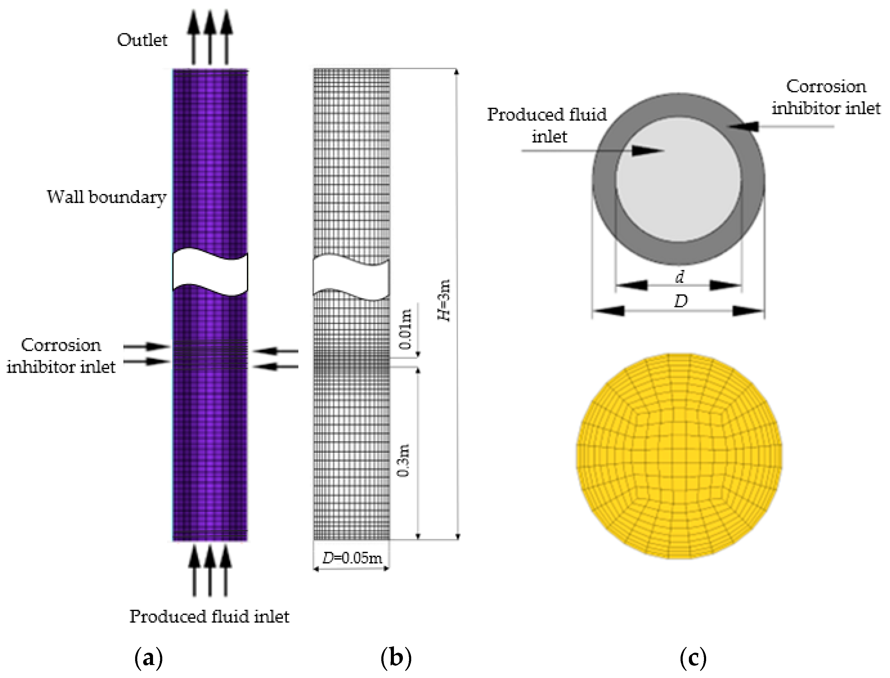
2.3.1. Computational Geometry

The schematic diagram of the tubing, casing and its supporting equipment of a self-flowing well is shown in Figure 1.

It is known from the injection process of corrosion inhibitor conducted in the typical Yanchang Oilfield that the corrosion inhibitor solution is usually injected from the casing at the wellhead, and then flows into the tubing through the annulus between the casing and tubing at the bottom of the well. Subsequently, a protective film can form at the inner wall of the tubing when the corrosion inhibitor solution is carried away by the produced fluid.

As shown in Figure 2, a simplified three-dimensional numerical model was established to simulate the vertical produced fluid-corrosion inhibitor solution flow in the tubing. The height of the tubing H is 3.0 m, and the corresponding inner diameter D is 0.05 m. The produced fluids flow from the bottom of the tubing and the corrosion inhibitors flow through an annular gap of 0.01 m at a distance of 0.3 m from the bottom of the tubing. The meshing of the model was performed using the multi-sweeping method. To resolve the corrosion inhibitor solution flow in a narrow annulus, a progressively finer mesh was taken near the tubing wall, as well as near the tubing inlet and its exit and the corrosion inhibitor inlet. The computational domain was meshed with hexahedral elements, which can not only reduce the number of volume elements, but also improve the solution accuracy and convergence.

2.3.2. Solution Setup

The model was numerically solved using the finite volume method and the SIMPLEC method was used to solve the momentum equations coupled with the pressure and velocity. Meanwhile, the momentum equations were discretized using the second-order upwind method, which can help to improve the accuracy of the solution. Transient simulations with sufficiently small time step (10⁻⁴ s) were performed. The Geo-Reconstruct scheme was applied to determine the interface shape. Convergence was judges based on the transport equation residuals and conservation of mass for each fluid. At the bottom inlet of the tubing, velocity boundary condition was applied and the produced fluid was set as the primary phase. At the outlet, a free outflow condition was used and a no-penetration and no-slip boundary condition was imposed on the impermeable tubing wall.

An imidazoline type oil-soluble corrosion inhibitor was selected in this numerical study, and the basic properties are shown in

Table 2. Basic properties of the imidazoline type oil-soluble corrosion inhibitor.

Density/(g/cm3)	Freezing Point/(°C)	pH	Dosage/(ppm)	Corrosion Rate/(mm/a)	Injection Method
20	−15	6–8	200	0.043	Continuous injection

. The density of the corrosion inhibitor solution measured is 20 g/cm³ at room temperature and the freezing point is −15 °C. The pH value was maintained between 6 and 8. Consistent with the production parameters in Yanchang Oilfield, continuous injection of 200 ppm dosage was recommended, which can reduce the corrosion rate in the wellbore to 0.043 mm/a.

A summary of the simulation condition was provided in

Table 3. Summary of the simulation condition.

Simulation Condition	Inlet 1 (Produced Fluid)		Inlet 2 (Corrosion Inhibitor)
	Water	Oil	Polymer Solution
Volume fraction, %	80	20	100
Velocity, m/s	0.05–1.5	0.05–1.5	0.1–0.9
Volume fraction of corrosion inhibitor, %	0	0	100
Viscosity, mPa·s	/	/	50–250

. The produced fluid was taken as one phase, and its property was determined by the corresponding components of water and oil. The volume fractions of water and oil at the inlet were identified as 80% and 20%, respectively, which is essentially consistent with the field data as shown in Table 1. The input superficial velocities of the water and oil are in the same range of 0.05–1.5 m/s, and the input superficial velocity of the corrosion inhibitor solution is kept in the range of 0.1–0.9 m/s. In addition, the viscosity of the polymer solution varies from 50 mPa·s to 250 mPa·s.

2.3.3. Grid Independence Verification

A mesh independence study was conducted to ensure that the mesh resolution does not significantly affect the results of the numerical simulation. To this aim, structured grids were used to discretize the computational space. The information of four numbers of elements are shown in

Table 4. Grid independence analysis on the inlet pressure and outlet flow velocity.

No.	Elements	Inlet Pressure, MPa	Outlet Flow Velocity, m/s
1	91,000	15.37	0.84
2	131,096	15.93	0.76
3	223,215	16.07	0.73
4	396,354	16.03	0.77

.

It can be found that the calculation accuracy increases with increasing the elements; however, the balance between the accuracy and calculation time needs to be taken into consideration. The deviations between the calculated inlet pressure, outlet flow velocity and the reference value (223,215 elements) are only approximately 0.2% and 5.1%; thus, the mesh of 396,354 elements can lead to relatively high simulation accuracy in a reasonable simulation time.

3. Results and Discussion

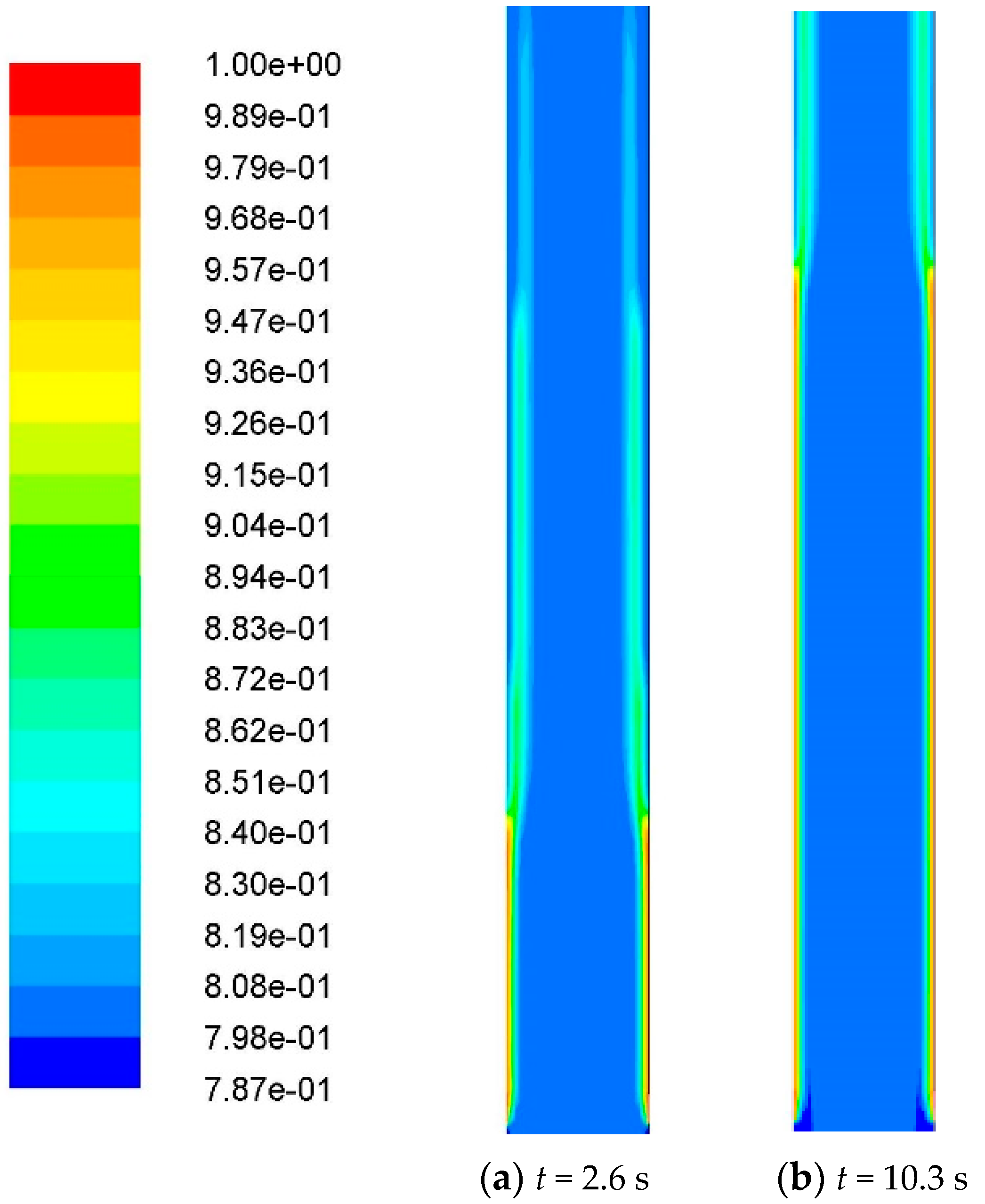
3.1. Effect of Calculation Time

The volume fractions of the corrosion inhibitor at different moments calculated using numerical simulation are shown in Figure 3. From the contours obtained at t = 2.6 s and t = 10.3 s, it is obvious that the corrosion inhibitor, which is carried by the produced fluid, flows upwards along the inner wall of the tubing. In addition, the corrosion inhibitor tends to diffuse to the center of the tubing gradually with time, and the volume fraction of the corrosion inhibitor near the inner wall slowly decreases.

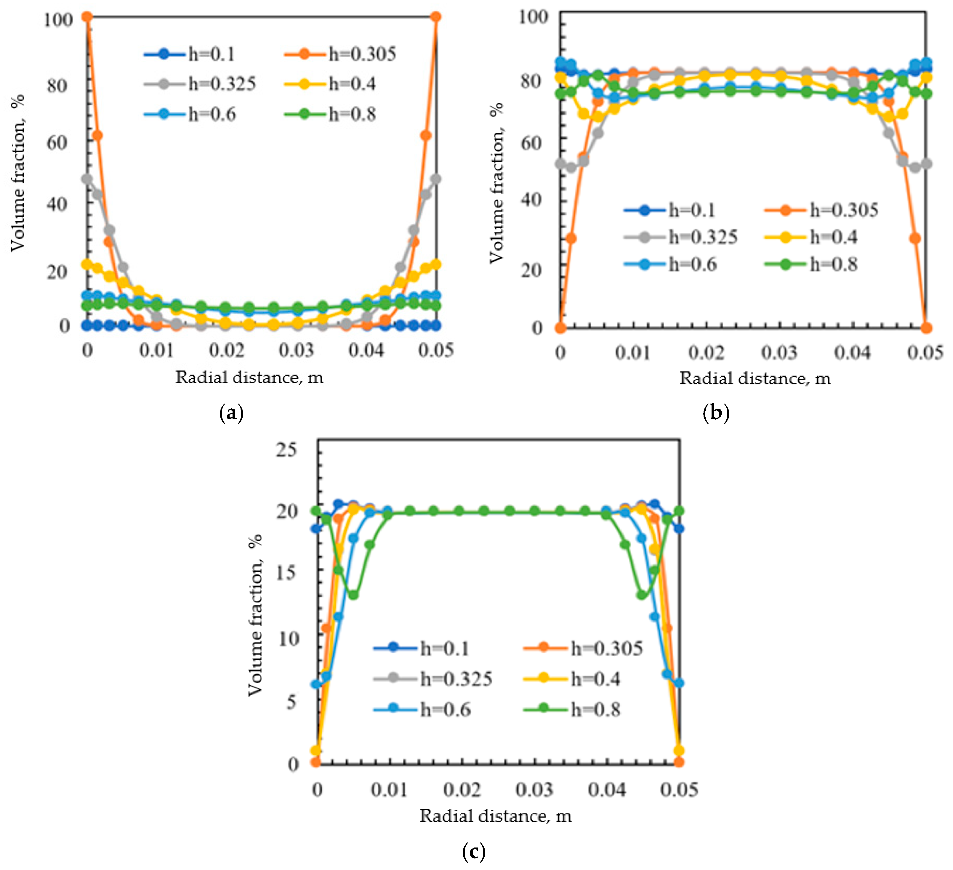
3.2. Effect of Tubing Height

Figure 4 shows the volume fractions of the corrosion inhibitor, water and oil at different tubing heights. It can be observed from Figure 4a that a stable annular flow of corrosion inhibitor can form along the tubing and the volume fraction varies with the increase in the tubing height. At a low tubing height (h = 0.1 m, lower than the corrosion inhibitor inlet), the sectional concentration of the corrosion inhibitor is always maintained at zero; correspondingly, the volume fractions of water and oil remain the same as the initial values of 80% and 20%, respectively. At a higher tubing height of 0.305 m, the volume fraction of the corrosion inhibitor at the tubing inner wall rapidly increases to 100%, but still remains zero at the tubing center. As the tubing height continues to increase, the volume fractions of the corrosion inhibitor at the tubing wall gradually decline; however, those fractions in the center of the tubing slightly increase. When the tubing height is higher than 0.8 m, the cross-sectional volume fraction of the corrosion inhibitor essentially maintains at approximately 10%. It is noted that the corrosion inhibitor injected through the annulus of tubing and casing can effectively form a certain thickness of corrosion inhibitor liquid film on the inner wall of the tubing, thus isolating the metallic tubing wall from the corrosive medium and mitigating the wellbore corrosion [31].

As shown in Figure 4b,c, the volume fractions of the water and oil remain the same as the input values at low tubing height of 0.1 m. With the increase in tubing height and injection of corrosion inhibitor, both the volume fractions of water and oil at the tubing inner wall decrease first and then gradually increase. It can be indicated that the maximum concentration of corrosion inhibitor occurs near the tubing inner wall, but not at the inner wall due to the diffusion effect of the corrosion inhibitor. When the tubing height is higher than 0.325 m, the volume fractions of water and oil essentially maintain at approximately 80% and 20%, respectively, which is consistent with the distribution of the corrosion inhibitor shown in Figure 4a. Furthermore, it is worth noting that when the height is higher than 0.8 m, both the water and oil volume fractions approach their lowest values. It can be explained that the corrosion inhibitor are concentrated near the tubing inner wall when it was injected from the inlet at a distance of 0.3 m from the tubing bottom. Furthermore, a produced fluid-corrosion inhibitor solution core annular flow can form, in which the produced fluid maintains in the center and the corrosion inhibitor solution in the annulus [32].

The distribution curves of volume fractions of the corrosion inhibitor at different tubing heights can be fitted with different functions and the results are shown in

Table 5. Fitting results of the corrosion inhibitor volume fraction curves at different tubing heights.

Tubing Height, m	Fitted Correlations of the Volume Fraction	R2	Variance	Standard Deviation
0.305	$\{\begin{array}{c}y=4047.3x^2-202.3x+0.9431 y>0\hfill \\ y=2.1\times {10}^{-5}\hspace{1em}\hspace{1em}\hspace{1em}\hspace{1em}\hspace{1em}\hspace{1em}\hspace{1em}y\le 0\hfill \end{array}$	0.95	0.003295	0.0574
0.325	$\{\begin{array}{c}y=1168.3x^2-58.413x+0.4827 y>0\hfill \\ y=2.1\times {10}^{-5}\hspace{1em}\hspace{1em}\hspace{1em}\hspace{1em}\hspace{1em}\hspace{1em}\hspace{1em}y\le 0\hfill \end{array}$	0.98	8.1 × 10−7	0.0009
0.4	$y=322.4x^2-16.12x+0.2067\hspace{1em}y>0$	0.94	0.001867	0.04321
0.6	$y=85.805x^2-4.2909x+0.1039\hspace{1em}y>0$	0.97	7.73 × 10−6	0.00278
0.8	$y=61.035x^2-3.04x+0.0715\hspace{1em}y>0$	0.97	7.24 × 10−6	0.00269

. At a tubing height of 0.305 m and 0.325 m, the volume fraction curves can be fitted with segmented functions, respectively. Both the correlation coefficients R² are larger than 0.95 and the corresponding RMSE values are less than 1.09 × 10⁻³. When the height is larger than 0.4 m, the corresponding curves can be fitted with quadratic polynomial functions. The parameters in each correlation are different; thus, the individual parameters a, b, c are again fitted as a function of the tubing height (Equation (20)).

$$y=a{x}^2-bx+c$$

(19)

$$\{\begin{array}{c}a=t{(h-m)}^n\\ b=t{(h-m)}^n\\ c=t{(h-m)}^n\end{array}$$

(20)

As shown in

Table 6. T-value test conducted on the fitting parameters in Equation (20).

Parameter		Fitted Parameters	Variance	Standard Deviation	T-Value	t-Test	Independent Distribution
a	t	30.1262	31.48	5.61111	5.36903	0.11723	0.99931
	m	0.29645	1.0 × 10−6	0.001	296.2949	0.00215	0.99822
	n	−1.02911	0.004	0.06352	−16.2003	0.03925	0.99973
b	t	1.50629	0.0786	0.28038	5.37228	0.11716	0.99931
	m	0.29645	1.0 × 10−6	0.001	296.3502	0.00215	0.99822
	n	−1.02914	0.004	0.06349	−16.2093	0.03923	0.99973
c	t	0.0447	5.336 × 10−6	0.00231	19.34401	0.03288	0.99467
	m	0.29281	5.388 × 10−7	7.34 × 10−4	399.1817	0.00159	0.98953
	n	−0.69195	0.000414	0.02034	−34.0122	0.01871	0.998

, the T-value test was conducted on the fitted parameters t, m, n in Equation (20) and reasonable fitted parameters were obtained with small standard deviations. All the independent distribution values are nearly close to 1. It can also be seen from Figure 5 that a good agreement was achieved between the calculated volume fractions of the corrosion inhibitor and the simulated ones, and the relative errors are essentially within ±20%. The correlations obtained can facilitate the rapid determination of the corrosion inhibitor distribution at different tubing heights.

3.3. Effect of Injection Rate of Corrosion Inhibitor

Figure 6 shows the effects of injection rate on the distribution of corrosion inhibitor on the tubing inner wall of h = 0.3, where the volume fractions of corrosion inhibitor can be clearly observed at different locations in the cross-section. The injection rate provides the radial velocity of corrosion inhibitor entering the tubing; thus, it greatly affects the radial distribution of corrosion inhibitor along the tubing. When the injection rate increases from 0.1 m/s to 0.9 m/s, the volume fraction of corrosion inhibitor very close to the tubing inner wall reduces from 47% to 31.1%, while the volume fraction in the center of the tubing increases to 6%. It can be seen that excessive radial velocity may cause the corrosion inhibitor to not easily adhere to the tubing inner wall, and a large amount of corrosion inhibitor is concentrated in the central area of the tubing at a large initial radial velocity. Therefore, an excessively large injection rate is not conducive to the corrosion inhibitor adherence to the tubing wall. Under the simulated conditions as mentioned before, the volume fraction of corrosion inhibitor in the tubing center tends to 0 at an inlet velocity of 0.1 m/s, the volume fraction close to the tubing inner wall reaches the highest of approximately 48% instead, which confirms that a more stable annular flow can be obtained.

In terms of corrosion inhibitor film formation only, the lower the injection rate, the better it is for the formation of corrosion inhibitor film on the tubing inner wall. However, at a low injection rate, a higher volume fraction near the inner wall can be obtained; however, the thickness of the corrosion inhibitor film is much smaller and the annular flow is also unstable. Therefore, properly increasing the injection rate is beneficial to maintaining the stability of the annular flow. In general, the flow pattern in the tubing mainly depends on the ratio of gravity to viscous force ($G/V=\frac{\Delta \rho g{D}^2}{\mu U}$). When the G/V ratio is small, namely the viscous force is dominant, it is easier to obtain an annular flow [33,34]. The value of G/V decreases with increasing the injection rate; thus, increasing the injection rate of corrosion inhibitor can improve the stability of the annular flow structure to a certain extent. On the whole, both the film quality of the corrosion inhibitor and stability of the annular flow need to be taken into account when determining the injection rate of corrosion inhibitor.

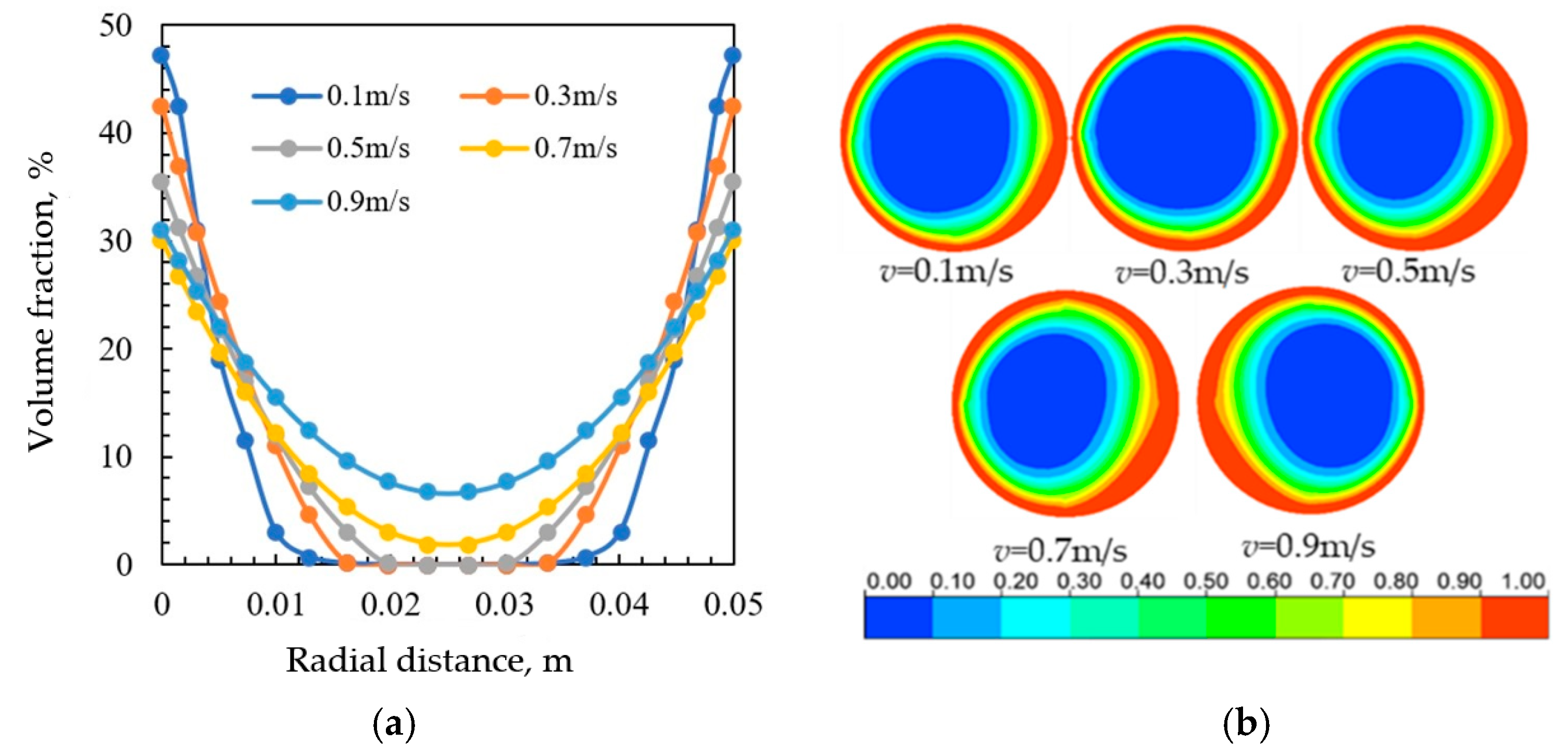
3.4. Effect of Produced Fluid Velocity

The effects of the produced fluid velocity on the distribution of corrosion inhibitor obtained in the simulations are shown in Figure 7. It can be observed that the corrosion inhibitor near the tubing inner wall migrates obviously to the center at low velocities of produced fluid, and its volume fraction reaches 9.4% at the radial distance of 16.2 mm. As the velocity continues to increase, the corrosion inhibitor is gradually squeezed by the produced fluid to the inner wall of the tubing. In Figure 7b, it can be observed that increasing the velocities of produced fluid leads to a higher volume fraction of corrosion inhibitor and a better protective film adhering to the tubing inner wall. At a low produced fluid velocity (v = 0.05 m/s), the corrosion inhibitor adhered to the inner wall of the tubing diffuses outward significantly and the maximum volume fraction of corrosion inhibitor near the inner wall is only 25%. When the produced fluid velocity reaches 1.0 m/s, the volume fraction rapidly increases to approximately 60%. Furthermore, a maximum volume fraction of 68% can be achieved when the produced fluid velocity increases to 1.5 m/s. The reason may be that the produced fluid velocity is high enough, while the velocity in the flow boundary layer near the wall is still very low (approaching 0); thus, a larger velocity gradient appears, which leads to more obvious diffusion of the corrosion inhibitor. Based on the phase diffusion equation, the velocity difference between the two phases is very important for the diffusion velocity [35,36]. Therefore, appropriately increasing the produced fluid velocity is beneficial to the corrosion inhibitor to adhering to the inner wall of the tubing. However, in turn, excessive velocity tends to wash away the protective film on the tubing inner wall [37]. An appropriate velocity is in the range of 1.0 m/s ≤ v ≤ 1.5 m/s under the entire simulation conditions in this work.

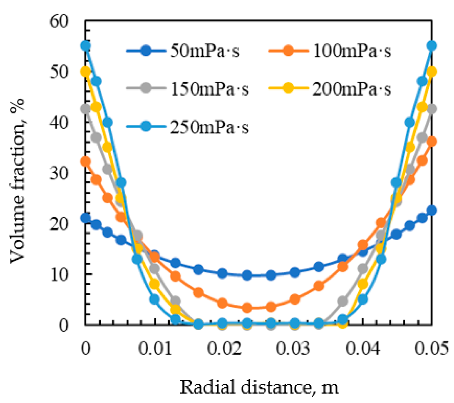
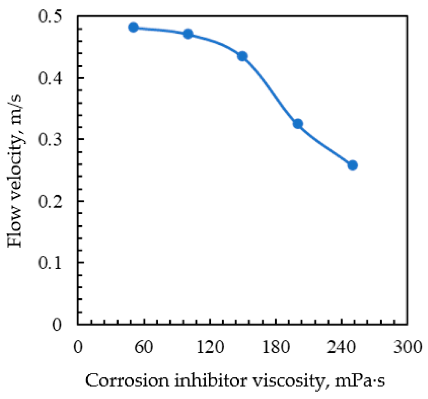
3.5. Effect of Corrosion Inhibitor Viscosity

Figure 8 demonstrates the effects of corrosion inhibitor viscosity on its distribution in the tubing. The inlet velocities of the produced fluid and corrosion inhibitor are fixed at 0.5 m/s and 0.1 m/s, respectively, and the viscosity of the corrosion inhibitor varies from 50 mPa·s to 250 mPa·s. It is found that the volume fraction of corrosion inhibitor near the tubing inner wall increases with the increase in the corrosion inhibitor viscosity. When the viscosity is less than 150 mPa·s, the volume fraction of corrosion inhibitor is sensitive to its viscosity. The volume fraction at the same radial distance increases by 34% when the corrosion inhibitor viscosity increases from 100 mPa·s to 150 mPa·s. As the viscosity continues to increase above 200 mPa·s, the increasing rate of the volume fraction of corrosion inhibitor on the tubing wall becomes moderate. This indicates that increasing the viscosity of the corrosion inhibitor adequately helps to enhance its adhesion on the tubing inner wall and also helps to protect the tubing against corrosion, which is consistent with the simulation results of corrosion inhibitor distribution in pipes obtained by Zhuo et al. [38].

However, excessive viscosity of corrosion inhibitor will also reduce its fluidity in the tubing. The comparison of the flow velocities of corrosion inhibitor on the inner wall of the tubing at different viscosities of corrosion inhibitor are shown in Figure 9. The inlet velocity of the corrosion inhibitor is relatively low compared to the velocity of the produced fluid, and the flow velocity of corrosion inhibitor is further reduced with the increase in its viscosity. As mentioned above, the increase in the corrosion inhibitor viscosity could lead to a more stable annular flow and a more ideal protective film adhering to the tubing inner wall. Nevertheless, when the corrosion inhibitor viscosity increases above 150 mPa·s, its flow velocity rapidly decreases; the increased velocity difference between the produced fluid and corrosion inhibitor solution will accelerate the diffusion of the corrosion inhibitor from the tubing inner wall to the center area. Hence, excessive viscosity of the corrosion inhibitor is not conducive to its adhesion to the inner wall of the tubing.

3.6. Injection Cycle of Corrosion Inhibitor

In the continuous injection process, a stable film of corrosion inhibitor can be formed on the entire inner wall of the tubing when the corrosion inhibitor is carried by the produced fluid to the wellhead. As the corrosion inhibitor continues to be injected, it will be continuously adhered to the tubing inner wall, thereby isolating the corrosive medium. In addition to the continuous injection process, intermittent injection is also applied in the oilfields. In this process, the corrosion inhibitor is continuously injected first, and a stable protective film forms due to the strong surface tension of corrosion inhibitor [39]. Then, the injection is stopped, and the concentration of corrosion inhibitor on the inner wall will gradually decrease under the continuous scouring of produced fluid from the bottom of the well. When the concentration of corrosion inhibitor is too low or the liquid film is completely damaged, the corrosion inhibitor will be injected again from the annulus between the casing and tubing. The intermittent injection process can significantly reduce the consumption of corrosion inhibitor and the load of injection equipment, which is an advanced technology for the refined and intelligent management of oil fields [40]. However, the injection cycle of intermittent injection is closely related to the quality of film formation on the tubing wall. Too frequent injections will waste chemicals and increase labor costs; however, if the injection interval is too long, the corrosion inhibitor film will be thinned by the produced fluid and the tubing steel will be exposed to the corrosive medium again. Therefore, the determination of an injection cycle is key to ensuring the film quality of the intermittent injection process [41].

Figure 10 illustrates distribution of corrosion inhibitor along the tubing inner wall at different moments after stopping injection. At the beginning, a complete film can still be observed on the inner wall (Figure 10a). After stopping injections for 5 h, the concentration of corrosion inhibitor in the upper part of the tubing remains unchanged; however, the concentration near the inlet begins to decrease and migrates to the center of the tubing (Figure 10b). With the injection stopping time further extended to 10 h, the concentration of corrosion inhibitor near the inner wall of the upper part of the tubing also begins to decrease, and the concentration near the inlet continues to decrease (Figure 10c). As shown in Figure 10e, the concentration on the inner wall near the inlet decreases to less than 10% after 20 h.

Figure 11 shows the volume fractions of corrosion inhibitor on the inner wall of the tubing of h = 0.3 m at different stopping times. It is found that the volume fraction on the inner wall decreases significantly at the initial stage of stopping injection, and it decreases by 62% within 10 h. Subsequently, the decreasing trend of the volume fraction gradually slows down with time, and it only decreases by 40% at 40 h. The volume fraction curve can be fitted using an exponential function with a correlation coefficient R² of 0.99. Based on the correlation established, the time of the minimum protective effect of the corrosion inhibitor on the inner wall of the tubing, namely the time when additional corrosion inhibitor needs to be supplemented, can be deduced. In this case, it is assumed that the corrosion inhibitor has no corrosion mitigation effect when its volume fraction is lower than 1%. When the volume fraction of corrosion inhibitor on the tubing inner wall near the inlet decreases to less than 1% after the injection is stopped for 3.5 days, it means that it is the time to have corrosion inhibitor re-injection; in addition, the minimum injection cycle can be roughly identified as 3.5 days.

The effective repair time of the corrosion inhibitor adsorption film is usually used as a method to determine the corrosion inhibitor injection cycle [42]; however, a considerable number of parameters are involved in the calculation process, which causes difficulty in achieving it. The abovementioned method for determining the corrosion inhibitor injection cycle is mainly based on the diffusion effect of produced fluid-corrosion inhibitor solution two-phase flow. In practical applications, the volume fraction of corrosion inhibitor will be affected by other factors, including pressure, temperature and wall roughness, etc. in the tubing. It is often difficult to take all the main factors into account. The injection cycle determined using the simulation method in this study may have some deviations from the true value; however, in general, it is a simple, feasible and relatively reliable method.

4. Conclusions

In this work, a three-dimensional numerical model for the tubing in the wellbore and the Eulerian two-fluid model and turbulence modelling method were combined to study the produced fluid-corrosion inhibitor solution two-phase flow and intermittent injection cycle of corrosion inhibitor. To the best of our knowledge, this is the first attempt to explore the distribution characteristics of corrosion inhibitor in a high water-cut oil well, which can provide new insights for the formulation of on-site wellbore corrosion prevention and control schemes in oil fields.

The main factors, including time, wellbore heights, injection rates, oil phase velocities and corrosion inhibitor viscosities, affecting the corrosion inhibitor distribution inside the tubing were investigated. Once the corrosion inhibitor solution was injected through the annulus of tubing and casing, a stable produced fluid-corrosion inhibitor solution annular flow can be maintained under appropriate conditions. With the increase in tubing height, a protective film of corrosion inhibitor adhered on the tubing inner wall can maintain for a long time. Empirical formulas for predicting the volume fraction of corrosion inhibitor at different tubing heights were obtained using the regression method and the relative errors between the calculated and simulated values are essentially within ±20%. Furthermore, a proper increase in injection rate of corrosion inhibitor can improve the stability of the annular flow structure; however, both the stability of the annular flow and film quality of the corrosion inhibitor are the two key factors determining the injection rate of corrosion inhibitor. Increasing the produced fluid velocity and reducing viscosity of corrosion inhibitor is conducive to the adhesion of corrosion inhibitor to the inner wall of the tubing. Moreover, the key to maintaining the integrity of the corrosion inhibitor film at the tubing inner wall is to determine an appropriate injection cycle. Based on the interphase diffusion effect, a feasible method for determining the injection cycle of corrosion inhibitor was proposed. The minimum corrosion inhibitor injection interval of 3.5 days was identified under the simulated conditions of this work.

References

1. Zeng, D.; Dong, B.; Zeng, F.; Yu, Z.; Tao, Y. Analysis of corrosion failure and materials selection for CO2-H2S gas well. J. Nat. Gas Sci. Eng. 2020, 86, 103734. [Google Scholar] [CrossRef]
2. Wang, R.; Luo, S. Grooving corrosion of electric-resistance-welded oil well casing of J55 steel. Corros. Sci. 2013, 68, 119–127. [Google Scholar] [CrossRef]
3. Abdel Ghany, N.A.; Shehata, M.F.; Saleh, R.M.; El Hosary, A.A. Novel corrosion inhibitor for acidizing oil wells. Mater. Corros. 2016, 68, 355–360. [Google Scholar] [CrossRef]
4. Huang, L.; Li, H.; Wu, Y. Comprehensive evaluation of corrosion inhibition performance and ecotoxicological effect of cinchona IIa as a green corrosion inhibitor for pickling of Q235 steel. J. Environ. Manag. 2023, 335, 117531. [Google Scholar] [CrossRef]
5. Medupin, R.O.; Ukoba, K.O.; Yoro, K.O.; Jen, T.C. Sustainable approach for corrosion control in mild steel using plant-based inhibitors: A review. Mater. Today Sustain. 2023, 22, 100373. [Google Scholar] [CrossRef]
6. Pan, C.; Chen, N.; He, J.; Liu, S.; Xu, P. Effects of corrosion inhibitor and functional components on the electrochemical and mechanical properties of concrete subject to chloride environment. Corros. Sci. 2020, 260, 119–124. [Google Scholar] [CrossRef]
7. Shamsa, A.; Barker, R.; Hua, Y.; Barmatov, E.; Hughes, T.; Neville, A. Impact of corrosion products on performance of imidazoline corrosion inhibitor on X65 carbon steel in CO2 environments. Corros. Sci. 2021, 85, 109423. [Google Scholar] [CrossRef]
8. Choi, H.; Song, Y.K.; Kim, K.Y.; Park, J.M. Encapsulation of triethanolamine as organic corrosion inhibitor into nanoparticles and its active corrosion protection for steel sheets. Surf. Coat. Technol. 2012, 206, 2354–2362. [Google Scholar] [CrossRef]
9. Javidi, M.; Chamanfar, R.; Bekhrad, S. Investigation on the efficiency of corrosion inhibitor in CO2 corrosion of carbon steel in the presence of iron carbonate scale. J. Nat. Gas Sci. Eng. 2019, 61, 1970205. [Google Scholar] [CrossRef]
10. Negm, N.A.; Tawfik, S.M.; Badr, E.A.; Abdou, M.I.; Ghuiba, F.M. Evaluation of some nonionic surfactants derived from vanillin as corrosion inhibitors for carbon steel during drilling processes. J. Surfactants Deterg. 2015, 18, 413–420. [Google Scholar] [CrossRef]
11. Bacca, K.R.G.; Lopes, N.F.; Marcolino, J.B.; Grasel, F.D.S.; Costa, E.M. Performance of Quebracho extract as eco-friendly corrosion inhibitor for SAE 1010 steel in the oil field environment. Mater. Corros. 2020, 71, 155–165. [Google Scholar] [CrossRef]
12. Gao, X.; Zhang, X.; Wang, J. Numerical simulation of corrosion inhibitor behavior. J. Drain. Irrig. Mach. Eng. 2017, 35, 50–55. [Google Scholar]
13. Rojas-Figueroa, A.; Fairuzov, Y.V. Numerical simulation of corrosion inhibitor transport in pipelines carrying oil-water mixtures. J. Energy Resour. Technol. 2002, 124, 239–245. [Google Scholar] [CrossRef]
14. Quentin, L.; Lamarque, N.; Hélie, J.; Legendre, D. On the spreading of high-pressure spray-generated liquid wall films. Int. J. Multiphas. Flow 2021, 139, 103619. [Google Scholar]
15. Liu, E.; Li, D.; Zhao, W.; Peng, S.; Chen, Q. Correlation analysis of pipeline corrosion and liquid accumulation in gas gathering station based on computational fluid dynamics. J. Nat. Gas Sci. Eng. 2022, 102, 104564. [Google Scholar] [CrossRef]
16. Liu, E.; Tang, H.; Zhang, Y.; Li, D.; Kou, B.; Liu, N.; Azimi, M. Experiment and numerical simulation of distribution law of water-based corrosion inhibitor in natural gas gathering and transportation pipeline. Petrol. Sci. 2023, in press. [Google Scholar] [CrossRef]
17. Jing, J.; Xiao, F.; Yang, L.; Wang, S.; Sun, J. Experimental and simulation study of atomization concentration of corrosion inhibitor in a gas pipe. J. Nat. Gas Sci. Eng. 2018, 49, 8–18. [Google Scholar] [CrossRef]
18. Farokhipour, A.; Mansoori, Z.; Saffar-Avval, M.; Ahmadi, G. 3D computational modeling of sand erosion in gas-liquid-particle multiphase annular flows in bends. Wear 2020, 450, 203241. [Google Scholar] [CrossRef]
19. Farhadian, A.; Rahimi, A.; Safaei, N.; Shaabani, A.; Alavi, A. A theoretical and experimental study of castor oil-based inhibitor for corrosion inhibition of mild steel in acidic medium at elevated temperatures. Corros. Sci. 2020, 175, 108–113. [Google Scholar] [CrossRef]
20. Khan, F.; Sudhakara, S.M.; Puttaigowda, Y.M.; Pushpanjali. Amide substituted zinc centered macrocyclic phthalocyanines for corrosion inhibition of mild steel in hydrochloric acid medium. Surf. Eng. Appl. Electrochem. 2022, 58, 613–624. [Google Scholar] [CrossRef]
21. Tarek, G.; Meftah, H.; Shiferaw, R. Experimental investigation of gas–oil–water phase flow in vertical pipes: Influence of gas injection on the total pressure gradient. J. Petrol. Explor. Prod. Technol. 2019, 9, 3071–3078. [Google Scholar]
22. Strazza, D.; Grassi, B.; Demori, M.; Ferrari, V.; Poesio, P. Core-annular flow in horizontal and slightly inclined pipes: Existence, pressure drops, and hold-up. Chem. Eng. Sci. 2011, 66, 2853–2863. [Google Scholar] [CrossRef]
23. Kouris, C.; Tsamopoulos, J. Concentric core-annular flow in a circular tube of slowly varying cross-section. Chem. Eng. Sci. 2000, 55, 9–30. [Google Scholar] [CrossRef]
24. Strazza, D.; Poesio, P. Experimental study on the restart of core-annular flow. Chem. Eng. Res. Des. 2012, 90, 1711–1718. [Google Scholar] [CrossRef]
25. Chen, K.P.; Bai, R.; Joseph, D.D. Lubricated pipelining. Part 3. Stability of core annular flow in vertical pipes. J. Fluid Mech. 1990, 214, 251–286. [Google Scholar] [CrossRef]
26. Kishan, P.A.; Dash, S.K. Numerical and experimental study of circulation flow rate in a closed circuit due to gas jet impingement. Int. J. Numeri. Method. Heat Fluid Flow. 2006, 16, 890–909. [Google Scholar] [CrossRef]
27. Anglart, H.; Nylund, O.; Kurul, N.; Podowski, M.Z. CFD prediction of flow and phase distribution in fuel assemblies with spacers. Nucl. Eng. Des. 1997, 177, 215–228. [Google Scholar] [CrossRef]
28. Abubakar, A.; Al, W.Y.; Al, W.T.; Al, H.A.R.; Al, A.A.; Eshrati, M. Effect of pipe diameter on horizontal oil-water flow before and after addition of drag-reducing polymer part I: Flow patterns and pressure gradients. J. Petrol. Sci. Eng. 2017, 153, 12–22. [Google Scholar] [CrossRef]
29. Joseph, D.D.; Renardy, M.; Renardy, Y. Instability of the flow of two immiscible liquids with different viscosities in a pipe. J. Fluid Mech. 1984, 141, 309–317. [Google Scholar] [CrossRef] [Green Version]
30. Blyth, M.G.; Lug, H.; Pozrikidis, C. Stability of axisymmetric core-annular flow in the presence of an insoluble surfactant. J. Fluid Mech. 2006, 548, 207–235. [Google Scholar] [CrossRef] [Green Version]
31. Askari, M.; Aliofkhazraei, M.; Jafari, R.; Hamghalam, P.; Hajizadeh, A. Downhole corrosion inhibitors for oil and gas production—A review. Appl. Surf. Sci. Adv. 2021, 6, 100128. [Google Scholar] [CrossRef]
32. Ghosh, S.; Mandal, T.K.; Das, G.; Das, P.K. Review of oil water core annular. Renew. Sust. Energ. Rev. 2009, 13, 1957–1965. [Google Scholar] [CrossRef]
33. Al-Aufi, Y.A.; Hewakandamby, B.N. Thin film thickness measurements in two phase annular flows using ultrasonic pulse echo techniques. Flow Meas. Instrum. 2019, 66, 67–78. [Google Scholar] [CrossRef]
34. Ooms, G.; Segal, A. A theoretical model for core-annular flow of a very viscous oil core and a water annulus through a horizontal pipe. Int. J. Multiphas. Flow 1983, 10, 41–60. [Google Scholar] [CrossRef]
35. Zhu, H.; Wang, W. Molecular simulation study on adsorption and diffusion behaviors of CO2/N2 in lignite. ACS Omega 2020, 5, 29416–29426. [Google Scholar] [CrossRef]
36. Zhong, Q.; Jin, M. Zein nanoparticles produced by liquid–liquid dispersion. Food Hydrocolloid. 2009, 23, 2380–2387. [Google Scholar] [CrossRef]
37. Jing, J.; Sun, J.; Huang, H.; Zhang, M.; Wang, C.; Xue, X.; Ullmann, A.; Brauner, N. Facilitating the transportation of highly viscous oil by aqueous foam injection. Fuel 2019, 251, 763–778. [Google Scholar] [CrossRef]
38. Zhuo, K.; Qiu, Y.; Zhang, Y.; Du, W. Numerical simulation of the distribution of corrosion inhibitors. Petrochem. Technol. 2020, 49, 576–581. [Google Scholar]
39. Jovancicevic, V.; Ramachandran, S.; Prince, P. Inhibition of CO2 corrosion of mild steel by imidazolines and their precursors. Corrosion 1999, 55, 449–455. [Google Scholar] [CrossRef]
40. Zhang, D.; Ma, F.; Wu, Y.; Dong, Z. Optimization of injection technique of corrosion inhibitor in CO2-flooding oil recovery. J. Southwest Petrol. Univ. (Sci. Technol. Ed.) 2020, 42, 103–109. [Google Scholar]
41. Frenier, W.W.; Wint, D.D. Multifaceted approaches for controlling top-of-the-line corrosion in pipelines. Oil Gas Facil. 2014, 3, 65–80. [Google Scholar] [CrossRef] [Green Version]
42. Zhang, J.; Du, M.; Yu, H.; Wang, N. Effect of molecular structure of imidazoline inhibitors on growth and decay laws of films formed on Q235 Steel. Acta Phys. Chim. Sin. 2009, 25, 525–531. [Google Scholar]
Figure 1. Schematic diagram of the tubing, casing and supporting equipment of a self-flowing well.
Sustainability 15 06289 g001
Figure 2. Geometry for the produced fluid-corrosion inhibitor solution flow simulation. (a) Mesh of partial geometry; (b) Longitudinal sectional grid of the tubing; (c) Cross section of the tubing.
Sustainability 15 06289 g002
Figure 3. Volume fractions of the corrosion inhibitor in the tubing at different moments.
Sustainability 15 06289 g003
Figure 4. Volume fractions of corrosion inhibitor, water and oil at different tubing heights. (a) Corrosion inhibitor; (b) Water; (c) Oil.
Sustainability 15 06289 g004
Figure 5. Comparison of simulated volume fractions of corrosion inhibitor with the simulated values at different tubing heights.
Sustainability 15 06289 g005
Figure 6. Effects of injection rate of corrosion inhibitor on its distribution in the tubing. (a) Volume fraction vs. radial distance at different injection rates; (b) Cross-sectional phase distribution at different injection rates.
Sustainability 15 06289 g006
Figure 7. Effects of produced fluid velocity on the distribution of corrosion inhibitor in the tubing. (a) Volume fraction vs. radial distance at different produced fluid velocities; (b) Cross-sectional phase distribution at different produced fluid velocities.
Sustainability 15 06289 g007
Figure 8. Effects of corrosion inhibitor viscosity on its distribution in the tubing at constant inlet velocities of the produced fluid and corrosion inhibitor.
Sustainability 15 06289 g008
Figure 9. Effects of corrosion inhibitor viscosity on its flow velocity in the tubing.
Sustainability 15 06289 g009
Figure 10. Distribution of corrosion inhibitor along the tubing inner wall at different moments after stopping injection.
Sustainability 15 06289 g010
Figure 11. The function of the volume fraction of corrosion inhibitor on the inner tubing wall at different stopping times.
Sustainability 15 06289 g011