A Hierarchical Framework of Decision Making and Trajectory Tracking Control for Autonomous Vehicles

Abstract

Most of the existing research in the field of autonomous vehicles (AVs) addresses decision making, planning and control as separate factors which may affect AV performance in complex driving environments. A hierarchical framework is proposed in this paper to address the problem mentioned above in environments with multiple lanes and surrounding vehicles. Firstly, high-level decision making is implemented by a finite-state machine (FSM), according to the relative relationship between the ego vehicle (EV) and the surrounding vehicles. After the decision is made, a cluster of quintic polynomial equations is established to generate the path connecting the initial position to the candidate target positions, according to the traffic states of the EV and the target vehicle. The optimal path is selected from the cluster, based on the quadratic programming (QP) framework. Then, the speed profile is generated, based on the longitudinal displacement–time graph (S–T graph), considering the vehicle motion state constraints and collision avoidance. The smoothed speed profile is created through another QP formulation, in the space created by the dynamic-programming (DP) method. Finally, the planned path and speed profile are combined and sent to the lower level control module, which consists of the linear quadratic regulator (LQR) for lateral trajectory tracking control, and a double PID controller for longitudinal control. The performance of the proposed framework was validated in a co-simulation environment using PreScan, MATLAB/Simulink and CarSim, and the results demonstrate that the proposed framework is capable of addressing most ordinary scenarios on a structured road, with reasonable decisions and controlling abilities.

1. Introduction

With the increasing development of sensor and communication engineering, the AV has been brought to the forefront, due to its great potential for improving traffic safety, efficiency and energy reduction [1,2]. A significant factor in the development of the AV has been the annual Defense Advanced Research Projects Agency (DARPA) Grand Challenge, from whence AV has received great interest from academia, governments and industry [3]. Among these groups, the topic of safety is always the highest priority, underlined by statistics revealing that more than 94% of traffic accidents are caused by human factors [4]. The advanced driving assistant system (ADAS)—which includes lane-keeping assistants, autonomous emergency braking and adaptive cruise-control technologies—with which AVs are equipped is capable of reducing the chances of traffic accidents, and of improving driving safety [5]. The core part of the technology in AVs typically includes perception, decision making, planning and control [6]. In this paper, we study the decision making, planning and controlling features of AVs, as the information from the perception and localization module is assumed to be satisfactory.

The perception module is responsible for retrieving information from the driving environment of the AV. With the progress of sensor fusion and communication technology, AVs equipped with vehicle-to-vehicle (V2V) or vehicle-to-infrastructure (V2I) systems are referred to as connected autonomous vehicles (CAVs). Through onboard sensors, CAVs are linked with one another, the infrastructure is able to share information and the data obtained have higher accuracy and a wider range [7].

The decision-making module, which is the indicator of the intelligence level of AVs, and which is deemed to be the “brain” of the autonomous driving system, is based on the obtained environmental information, and ensures driving safety and comfort. The typical functions of the decision-making module include task planning, global route planning, decision making and local motion planning. Task planning can be considered a typical driving operation-scheduling problem, and global route planning is responsible for planning the rough driving trajectory which connects the start and end points in the road network. The trajectory obtained from global route planning only determines the road on which the vehicle should drive; hence, the smoothness of the trajectory is not guaranteed to guide the vehicle at the local motion level.

The decision-making module, which is also called the behavior-planning module, is always applied to determine driving behavior at a micro-level. Typical driving behaviors on a structured road include nudging, side passing, lane changing, yielding, overtaking, car-following and stopping. During the process of decision making, safety, legitimacy, comfort and efficiency are the indispensable elements that should be considered. The decision-making process is always categorized into rule-based and learning-based methods. The FSM method is a representative model in the rule-based category, which has an interpretable and simple structure based on if-then-else logic, and on the small size of the tuning parameters [8]. A hierarchy state machine was proposed in [9], which addresses the lane-changing decisions for AVs, and a heuristic-based FSM was proposed in [10] for evaluating safety regions and generating reasonable driving behavior. For learning-based methods, deep learning, reinforcement learning and inverse reinforcement learning are usually applied. A decision method based on the attention mechanism was proposed in [11], which addresses decision making in dense traffic environments. Some researchers have applied the long short-term memory (LSTM) neural network and conditional random field (CRF) to generate human-like decisions that increase lane-changing success rates [12,13]. For the reinforcement learning and inverse-reinforcement-learning methods, the research in [14] proposed a reinforcement Q-learning method based on rewarding and update functions for decision making. For highway-road simulation environments, the research in [15] proposed an inverse reinforcement learning (IRL) approach, using Deep Q-Networks to extract the rewards in problems with large-state spaces; the simulation results showed that the simulated agent could generate collision-free motions and perform human-like lane-changing behavior. However, the game-theory method has always been applied in the decision-making field, by modeling the interaction behaviors between AVs as either cooperative or non-cooperative games; further details can be found in [16,17,18].

With regard to local motion planning, graph search methods from the robotics field are widely used, including the A* method [19] and its variants, i.e., weighted A*, anytime A*, anytime repairing A* and anytime dynamic A* [20]; the D* method [21] and its variants, i.e., focused D* and D* lite [22]; and the rapid-exploring random tree method (RRT) and its variants, i.e., RRT* [23]. However, the smoothness of the path cannot be guaranteed by the graph search method. Some other popular methods are utilized to address this problem, such as potential field algorithms [24], parametric and semi-parametric methods (Bézier curves [25], the polynomial method [26], sigmoid functions [27], the spline-based method [28]) and numerical optimization approaches [29,30].

Trajectory tracking control has always been widely studied, and can be decoupled into longitudinal and lateral control. The lateral tracking control is responsible for following the planned trajectory, while in the longitudinal direction, the task is to track the planned speed profile. Commonly used trajectory tracking control methods include pure pursuit control [31], proportional integral derivative (PID) control [32], fuzzy logic control [33], sliding mode control [34] and LQR control [35]. As a typical strategy, model predictive control has also been studied by many researchers [36,37,38,39,40].

As mentioned above, the AV applies the decision made by the decision-making module based on the perception module to plan a feasible trajectory that reflects the expected driving behavior, which reacts to the dynamic environment. Then, the trajectory is sent to the control module and the actuators on the AV are controlled to follow the trajectory while considering constraints such as vehicle dynamics, safety and comfort. However, most studies consider the decision-making, planning and control modules as separate parts, rather than in an integrated manner.

Based on the fact that the framework proposed in this paper integrates the decision-making, trajectory-planning and control modules, it has the following characteristics:

(1)

The framework considers that the driving environment consists of multi-lane curved roads and multiple surrounding vehicles.

(2)

The FSM is utilized to determine the reasonable driving maneuver based on the relative safe distance and speed between the EV and surrounding vehicles under the constrained traffic conditions.

(3)

A cluster of quintic polynomial equations is established to generate the path connecting the initial position and the candidate target positions according to the traffic states of the EV and target vehicle.

(4)

The S–T graph and DP framework are applied to create the searching space for the speed profile.

(5)

The QP method is used to select the optimal path and speed profile under the constrained searching space.

(6)

The LQR controller and a double PID controller are responsible for the lateral and longitudinal tracking control, respectively.

2. Overall Structure of the Framework

A typical driving scenario is shown in Figure 1. The vehicles surrounding the EV considered in this paper include the current-lane front vehicle (CF), left-lane front vehicle (LF), left-lane rear vehicle (LR), right-lane front vehicle (RF) and right-lane rear vehicle (RR). The road considered in this paper has three lanes by default and the driving behavior is an element from a finite set {car following, free driving, left lane change, right lane change}. If the driving condition is the same for the left lane and right lane, the EV is expected to perform a left-lane change since the left lane is supposed to allow for a higher velocity.

The overall structure of the framework is shown in Figure 2. The framework is a hierarchical structure which consists of a sensor system, decision-making module, trajectory-planning module and control module. At the top, the sensor system equipped on the AV is assumed to be ideal. The required vehicle state information such as positions, velocities, accelerations and headings of the EV and surrounding vehicles can be obtained and broadcast to each other.

The decision-making module is implemented by an FSM, which is responsible for adopting reasonable driving behavior according to the relationship between the EV and the surrounding vehicles. The relative distance and velocity are used to judge whether the adjacent lane is safe, which is the criterion for potentially changing lanes. After the reasonable decision signal is made, the target vehicle is also available and the decision signal is sent to the planning module, which is mainly responsible for trajectory generation. The starting point and ending points are determined according to the decision made and the position of the target vehicle. Then, a cluster of the trajectories is generated by the quintic polynomials that connect the starting point and ending points, from which the optimal one is selected based on the cost function of each trajectory. After that, the speed profile is generated according to the S–T graph formulated under the constrained driving environment. The planning module works in the Frenet frame and coordinate transformation is applied to transform the trajectory, combining the local path and the speed profile into the Cartesian frame.

For the controller layer, the longitudinal and lateral control are implemented by an LQR and a double PID controller, respectively. The LQR controller is applied for tracking the planned trajectory in the lateral direction, and the PID controller with the inverse model is used for tracking the trajectory in the longitudinal direction while keeping a safe distance from the front vehicle and the desired velocity as much as possible by determining the required throttle opening or master cylinder pressure of CarSim. Finally, the EV is controlled by the framework to perform reasonable driving behavior and track the planned trajectory under the constrained driving environment.

3. Decision-Making Procedure

The decision-making procedure is implemented using an FSM algorithm in Stateflow to make reasonable and safe driving-behavior decisions according to the relationship between the EV and the other surrounding vehicles. The FSM is shown in Figure 3; the input to the FSM is the surrounding vehicles’ information and the output is the desired driving state based on the current driving conditions.

The decision is made according to the information of the surrounding vehicles, such as whether the front vehicle in the current lane is slower than the desired speed; the lane-changing decision or car-following decision is made according to the safe distance between the EV and the surrounding vehicles. The criterion for judging the safe distance is based on the longitudinal safe distance described in the RSS model, which was first introduced in [41]. The longitudinal safe distance is described as follows:

$$d_{lon}^s=max(0,v_r\rho +\frac{1}{2}{a}_{acc,max}{\rho }^2+\frac{{(v_r+a_{acc,max}\rho )}^2}{2a_{brake,min}}-\frac{v_f^2}{2a_{brake,max}})$$

(1)

where $v_f$ and $v_r$ are the velocity of the front and rear vehicles, respectively; $\rho$ is the maximum response time that the rear vehicle may take to initiate the required braking [42]; $a_{acc,max}$ is the maximum acceleration of the rear vehicle; and $a_{brake,min}$ and $a_{brake,max}$ are the minimum and maximum braking rates of the rear vehicle and front vehicle, respectively. If the adjacent lanes’ safe distances are satisfied, then the EV is able to perform the lane-changing behavior, and if that is not the case, the safe distance will also take effect in the car-following scenarios. The detailed description and the graphic representation of the RSS safe distance can be found in [43].

There are four driving states (car following, free driving, left lane change and right lane change) and six transition conditions ($C_1,C_2,C_3,C_4,C_5$ and $C_6$) in Figure 3. Here, the assumption that the left lane will always have a higher speed limit is made, so if there is a lane-changing need the left-lane-changing safe conditions will be verified first. The transition conditions that are used for generating driving states are described in

Table 1. Transition condition description.

Transition Condition	Description
$C_1$	Faster target vehicle or safe distance is satisfied
$C_2$	Desired speed is not satisfied
$C_3$	Left lane is safe
$C_4$	Right lane is safe
$C_5$	Left lane change is complete
$C_6$	Right lane change is complete

. The target vehicle described in the transition condition $C_1$ means the front vehicle under different driving states (e.g., left front vehicle for left lane changing state, same-lane front vehicle for car-following state and right front vehicle for right-lane-changing state). The output state of the FSM will be transmitted into the following trajectory planning module.

4. Trajectory Planning

After the decision is made, the next step is to plan a reasonable trajectory, which consists of a local path and a speed profile for the trajectory-tracking controller. In this study, the path–speed decoupling method is used, which will reduce the complexity of the trajectory-planning task.

The trajectory-planning module includes a reference-line generation module, path-planning module and speed-profile generation module. First, the reference line is a set of waypoints that are extracted from the lane centerline and smoothed by the smoothness cost function. The reference line forms the basis for the trajectory planning since it will determine the projection of the EV and construct the Frenet frame. In the path-planning module, the lane-changing target points are generated based on the target-point selection mechanism according to the current motion status of the EV and LF. Then, quintic polynomials are used for connecting the starting points and target points and the optimal path is selected based on the designed cost function. In the speed-profile generation module, the S–T graph space is constructed based on the optimal path for modeling the motion status of the surrounding environment, after which the S–T space is sliced by the sampling points in both S and T dimensions and the rough dynamic programming solution is obtained by calculating the cost for each sampling point. Finally, a smoothed speed profile is obtained through the QP framework by considering the constraints and the fact that a collision may occur during the lane-changing process. The optimal trajectory is the combination of the optimal path and the speed profile, which will be sent to the control layer for tracking.

4.1. Reference-Line Generation

Under the structured road environments, there is always a global path to guide the vehicle driving and the lane centerline is a common choice. The generation of the reference line relies on the position information of a series of waypoints, which are sampled from the lane centerline with the same interval. However, the sampled waypoints cannot be used as a whole if the reference line is too long, since this will increase the cost of determining the projections of the vehicle and obstacle positions relative to the centerline. In addition, there may be several projections of the vehicle onto the reference line and the centerline does not always have continuous curvature, which poses difficulties for the subsequent planning and controlling modules.

The plan is first to find the location point in the centerline waypoint set that has the smallest distance to the vehicle position; then, from this point, we search backward and forward in the set to create a subset of waypoints and, finally, apply the smoothing method to this subset to create a smoothed waypoint set; this is termed as the reference line. The problem is how to find the location point efficiently and it is not wise to consider all the waypoints in the original set in each planning period. Here, a hot-start and early-stop mechanism is applied to facilitate the efficiency of the algorithm. The algorithm used to find the location point is shown in Algorithm 1.    

Algorithm 1: Finding location points array

Input :       The vehicle position information array $vehiclePositionArray$;       The original waypoints array $waypointsArray$;       The global variable denotes first run of algorithm $isFirst$;       The global array denotes previous period location point index $previousPointsIndexArray$; Output:       Location point index array $pointsIndexArray$;       Location point array $pointsArray$; 1  initialize $pointsIndexArray$ and $pointsArray$; 2  if $isFirst$ then 3       $isFirst=False$; 4       initialize $lastPointsIndexArray$; 5       for $i=1:length\left(vehiclePositionArray\right)$ do 6        $minimumDistance=+\infty$; 7        $consecutiveIncreaseCount=0$; 8        for $j=1:length\left(wayPointsArray\right)$ do 9         $distance=$        $calculateDistance\left(vehiclePositionArray\right[i],wayPointsArray[j\left]\right)$; 10         if $distance<minimumDistance$ then 11            $minimumDistance=distance$; 12            $pointsIndexArray\left[i\right]=j$; 13            $consecutiveIncreaseCount=0$; 14         else 15            $consecutiveIncreaseCount=consecutiveIncreaseCount+1$; 16         end 17         if $consecutiveIncreaseCount>increaseThreshold$ then 18            $break$; 19         end 20        end 21        $pointsArray\left[i\right]=waypointsArray\left[pointsIndexArray\right[i\left]\right]$; 22       end 23       $previousPointsIndexArray=pointsIndexArray$; 24  else 25       for $i=1:length\left(vehiclePositionArray\right)$ do 26        $j=previousPointsIndexArray\left[i\right]$; 27        the rest of the process is the same as the isFirst run branch; 28       end 29  end

In Algorithm 1, the $vehiclePositionArray$ contains the vehicle position information in the Cartesian frame, while the $wayPointsArray$ contains the lane centerline information in the Frenet frame. The global variable $isFirst$ is used to decide whether the last period result is adopted. However, since it is not efficient to traverse all the waypoints to calculate the distance, once a minimum location point is found it will continue to search for the next $increaseThreshold$ waypoints to verify the property. If another minimum location point is acquired during the process, the variable $consecutiveIncreaseCount$ is cleared to zero and the whole process is repeated.

Next, based on the location point with index $lx$ in the $pointsArray$, we search backward $N_b$ and forward $N_f$ points, respectively, to create the subset of waypoints. The subset is smoothed by the following QP framework to create the local reference line:

$$\begin{array}{cc}\hfill & J_{smooth}=w_s\sum _{i=lx-N_b}^{lx+N_f-2}\left\{{(x_i+x_{i+2}-2x_{i+1})}^2+{(y_i+y_{i+2}-2y_{i+1})}^2\right\}\hfill \\ \hfill & +w_c\sum _{i=lx-N_b}^{lx+N_f-1}\left\{{(x_i-x_{i+1})}^2+{(y_i-y_{i+1})}^2\right\}+w_g\sum _{i=lx-N_b}^{lx+N_f}\left\{{(x_i-x_{ir})}^2+{(y_i-y_{ir})}^2\right\}\hfill \end{array}$$

(2)

where $x_r$ and $y_r$ are the coordinates of the original waypoints, $w_s$ is the weight for curvature, $w_g$ is the weight for controlling the deviation from the original waypoints and $w_c$ is used for controlling the compactness of the points in the set. The objective function in (2) is readily transformed into the standard QP form.

4.2. Frenet Frame and Transformation

The Frenet frame, which is also known as the curvilinear frame, is prevalent in the planning of the on-road trajectory frame [44]. An evident merit is that any type of road in the Cartesian frame can be transformed into a straight counterpart in the Frenet frame. Furthermore, it will relieve the difficulty of the planning and controlling task by decoupling the task into independent ones in longitudinal and lateral directions [45]. Moreover, it is relatively simple to calculate the deviation of the vehicle from the lane centerline and the driving distance along the lane centerline under the Frenet frame.

The planned trajectories under the Frenet frame should be converted back into the Cartesian frame for the controlling task. In the Frenet frame constructed based on the reference line, the longitudinal direction is supposed to be the direction along the reference line, while the lateral direction is supposed to be the direction perpendicular to the longitudinal direction.

Limited by the properties of vehicle kinematics, dynamics and road geometry, the actual driving trajectory is rather different from the reference trajectory. In the Cartesian frame, the vehicle motion state can be described as $[\overrightarrow{r_h},{\theta }_h,{\kappa }_h,\overrightarrow{v_h},\overrightarrow{a_h}]$. Here, $\overrightarrow{r_h}=(x,y)$ is the vehicle’s position, ${\theta }_h$ is the heading angle, ${\kappa }_h$ is the curvature, $\overrightarrow{v_h}$ is the velocity vector of the vehicle’s center of mass (COM) and $\overrightarrow{a_h}$ is the acceleration vector. Let the unit direction vector of the velocity vector of the vehicle’s COM $\overrightarrow{{\tau }_h}$ and its unit normal vector be $\overrightarrow{n_h}$.

In the Frenet frame, $\overrightarrow{r_r}=(x_r,y_r)$ is the position vector of the projection point P of the vehicle position Q. The motion state of the vehicle is expressed as $[s,\dot{s},\ddot{s},l,\dot{l},\ddot{l},l^{\prime },l^{″}]$, where s is the longitudinal displacement, $\dot{s}$ is the longitudinal velocity, $\ddot{s}$ is the longitudinal acceleration, l is the lateral displacement, $\dot{l}$ is the lateral velocity, $\ddot{l}$ is the lateral acceleration, $l^{\prime }$ is the first derivative of the lateral displacement with respect to the arc length and $l^{″}$ is the second derivative of the lateral displacement with respect to the arc length. Let $\overrightarrow{{\tau }_r}$, $\overrightarrow{n_r}$ and $\overrightarrow{\dot{s}}$ denote the unit tangent vector, unit normal vector and velocity vector, respectively. Moreover, $\Delta \theta ={\theta }_h-{\theta }_r$. All the above descriptions are expressed in Figure 4.

From Figure 4, the following equations can be obtained and will be applied later:

$$\overrightarrow{\dot{r_h}}=\overrightarrow{v_h}=\left|{\overrightarrow{v}}_h\right|{\overrightarrow{\tau }}_h$$

(3)

$$\overrightarrow{\dot{r_r}}=\frac{\mathrm{d}\overrightarrow{r_r}}{\mathrm{d}t}=\frac{\mathrm{d}\overrightarrow{r_r}}{\mathrm{d}s}\frac{\mathrm{d}s}{\mathrm{d}t}=\overrightarrow{{\tau }_r}\dot{s}$$

(4)

$$\overrightarrow{\dot{{\tau }_h}}=\frac{\mathrm{d}\overrightarrow{{\tau }_h}}{\mathrm{d}t}=\frac{\mathrm{d}\overrightarrow{{\tau }_h}}{\mathrm{d}{s}_h}\frac{\mathrm{d}{s}_h}{\mathrm{d}t}={\kappa }_h\overrightarrow{n_h}\left|\overrightarrow{v_h}\right|$$

(5)

$$\overrightarrow{\dot{n_h}}=\frac{\mathrm{d}\overrightarrow{n_h}}{\mathrm{d}t}=\frac{\mathrm{d}\overrightarrow{n_h}}{\mathrm{d}{s}_h}\frac{\mathrm{d}{s}_h}{\mathrm{d}t}=-{\kappa }_h\overrightarrow{{\tau }_h}\left|\overrightarrow{v_h}\right|$$

(6)

$$\overrightarrow{\dot{{\tau }_r}}=\frac{\mathrm{d}\overrightarrow{{\tau }_r}}{\mathrm{d}t}=\frac{\mathrm{d}\overrightarrow{{\tau }_r}}{\mathrm{d}s}\frac{\mathrm{d}s}{\mathrm{d}t}={\kappa }_r\overrightarrow{n_r}\dot{s}$$

(7)

$$\overrightarrow{\dot{n_r}}=\frac{\mathrm{d}\overrightarrow{n_r}}{\mathrm{d}t}=\frac{\mathrm{d}\overrightarrow{n_r}}{\mathrm{d}s}\frac{\mathrm{d}s}{\mathrm{d}t}=-{\kappa }_r\overrightarrow{{\tau }_r}\dot{s}$$

(8)

$$\overrightarrow{a_h}=|\overrightarrow{\dot{v_h}}|\overrightarrow{{\tau }_h}+{\kappa }_h{|\overrightarrow{v_h}|}^2\overrightarrow{n_h}$$

(9)

The lateral displacement l can be expressed as:

$$l=(\overrightarrow{r_h}-\overrightarrow{r_r})·\overrightarrow{n_r}$$

(10)

By taking the derivatives of both sides of the equation $\overrightarrow{r_r}+l\overrightarrow{n_r}=\overrightarrow{r_h}$ and combining (3), (4), (7) and (8) with it, we obtain:

$$\dot{s}\overrightarrow{{\tau }_r}+l(-{\kappa }_r\dot{s}\overrightarrow{{\tau }_r})+\dot{l}\overrightarrow{n_r}=\overrightarrow{v_h}$$

(11)

Taking the dot product on both sides of (11) by $\overrightarrow{n_r}$, we obtain:

$$\dot{l}=\overrightarrow{v_h}·\overrightarrow{n_r}$$

(12)

Taking the dot product on both sides of (11) by $\overrightarrow{{\tau }_r}$, we obtain:

$$\dot{s}=\frac{\overrightarrow{v_h}·\overrightarrow{{\tau }_r}}{1-{\kappa }_{r}l}$$

(13)

Combining the definition of $l^{\prime }$ and Equations (12) and (13), $l^{\prime }$ can be obtained from the following equation:

$$l^{\prime }=\frac{\mathrm{d}l}{\mathrm{d}s}=\frac{\mathrm{d}l}{\mathrm{d}t}\frac{\mathrm{d}t}{\mathrm{d}s}=\frac{\dot{l}}{\dot{s}}=(1-{\kappa }_{r}l)\frac{\overrightarrow{v_h}·\overrightarrow{n_r}}{\overrightarrow{v_h}·\overrightarrow{{\tau }_r}}$$

(14)

Taking the derivative of Equation (13), we obtain $\ddot{s}$ as follows:

$$\ddot{s}=\frac{\mathrm{d}\dot{s}}{\mathrm{d}t}=\frac{\overrightarrow{a_h}·\overrightarrow{{\tau }_r}}{1-{\kappa }_{r}l}+\frac{{\dot{s}}^2}{1-{\kappa }_{r}l}({\kappa }_r^{\prime }l+2{\kappa }_r{l}^{\prime })$$

(15)

Taking the derivative of Equation (12) and taking into account (8), we obtain:

$$\ddot{l}=\overrightarrow{a_h}·\overrightarrow{n_r}-{\kappa }_r(1-{\kappa }_{r}l){\dot{s}}^2$$

(16)

Since $\ddot{l}=\frac{\mathrm{d}\dot{l}}{\mathrm{d}t}=\frac{\mathrm{d}\left(l^{\prime }\dot{s}\right)}{\mathrm{d}t}=\frac{\mathrm{d}{l}^{\prime }}{\mathrm{d}t}\dot{s}+l^{\prime }\ddot{s}=\frac{\mathrm{d}{l}^{\prime }}{\mathrm{d}s}\frac{\mathrm{d}s}{\mathrm{d}t}\dot{s}+l^{\prime }\ddot{s}=l^{″}{\dot{s}}^2+l^{\prime }\ddot{s}$, $l^{″}$ can be expressed as:

$$l^{″}=\frac{\ddot{l}-l^{\prime }\ddot{s}}{{\dot{s}}^2}$$

(17)

From Equations (12) and (13), we can obtain:

$$|\overrightarrow{v_h}|sin\Delta \theta =\dot{l}$$

(18)

$$|\overrightarrow{v_h}|cos\Delta \theta =(1-{\kappa }_{r}l)\dot{s}$$

(19)

$$tan\Delta \theta =\frac{\dot{l}}{(1-{\kappa }_{r}l)\dot{s}}=\frac{l^{\prime }}{1-{\kappa }_{r}l}$$

(20)

The expression of $\overrightarrow{v_h}$ and ${\theta }_h$ can be obtained from (18)–(20):

$${\theta }_h={\theta }_r+arctan(\frac{l^{\prime }}{1-{\kappa }_{r}l})$$

(21)

$$|\overrightarrow{v_h}|={[{\dot{l}}^2+{(1-{\kappa }_{r}l)}^2{\dot{s}}^2]}^{\frac{1}{2}}$$

(22)

Then, $\overrightarrow{{\tau }_h}$ and $\overrightarrow{n_h}$ are expressed as:

$$\overrightarrow{{\tau }_h}=(cos{\theta }_h,sin{\theta }_h)$$

(23)

$$\overrightarrow{n_h}=(-sin{\theta }_h,cos{\theta }_h)$$

(24)

Following the same style of $\overrightarrow{v_h}$ by considering (15) and (16), $\overrightarrow{a_h}$ can be expressed as follows:

$$|\overrightarrow{a_h}|={\left\{{[\ddot{l}+{\kappa }_r(1-{\kappa }_{r}l){\dot{s}}^2]}^2+{[\ddot{s}(1-{\kappa }_{r}l)-{\dot{s}}^2(k_r^{\prime }l+2{\kappa }_r{l}^{\prime })]}^2\right\}}^{\frac{1}{2}}$$

(25)

$${\theta }_{a_h}={\theta }_r+arctan(\frac{\ddot{l}+{\kappa }_r(1-{\kappa }_{r}l){\dot{s}}^2}{\ddot{s}(1-{\kappa }_{r}l)-{\dot{s}}^2({\kappa }_r^{\prime }l+2{\kappa }_r{l}^{\prime })})$$

(26)

Finally, by taking the dot product on both sides of (9), we can obtain ${\kappa }_h$

$${\kappa }_h=\frac{\overrightarrow{a_h}·\overrightarrow{n_h}}{|\overrightarrow{v_h}{|}^2}$$

(27)

4.3. Quintic Polynomial

The trajectory planned for the lane-changing scenarios should be simple, safe and comfortable. For lateral control, the vehicle is supposed to follow the expected trajectory as close as possible, while in longitudinal control the vehicle is supposed to follow the target speed.

Typically, the indicator used for measuring the comfort and safety is jerk, which is the derivative of the acceleration. A high jerk value means the passengers will experience discomfort. Suppose p is the system to be calculated; then, for any time interval $[t_0,t_1]$, the process by which the system evolves from $[p\left(t_0\right),\dot{p}\left(t_0\right),\ddot{p}\left(t_0\right)]$ to the target state $[p\left(t_1\right),\dot{p}\left(t_1\right),\ddot{p}\left(t_1\right)]$ can be expressed as a one-dimensional integrator system [46]:

$$\dot{f}\left(t\right)=\left[\begin{array}{ccc}0& 1& 0\\ 0& 0& 1\\ 0& 0& 0\end{array}\right]f\left(t\right)+\left[\begin{array}{c}0\\ 0\\ 1\end{array}\right]\stackrel{⃛}{p}\left(t\right)$$

(28)

where $f\left(t\right)={[p\left(t\right),\dot{p}\left(t\right),\ddot{p}\left(t\right)]}^T$ and $\stackrel{⃛}{p}\left(t\right)$ denotes jerk.

It is proven in [46] that for the system in (28), the optimal trajectory sequence based on jerk exists in the set of quintic polynomials, and there exists a solution in the set that is capable of minimizing the cost function as follows:

$$J_{p_{\left(t\right)}}={\int }_{t_0}^{t_1}{\stackrel{⃛}{p}}^2\left(t\right)\mathrm{d}t$$

(29)

On a structured road, the AV is expected to move along the road either with the desired speed or the lane speed limit if there are no requirements (slow-moving preceding vehicle or obstacles) to change the current movement status. Otherwise, the vehicle needs to perform obstacle avoidance and lane-changing maneuvers. Similar to [47], the lateral trajectory planning in this study adopts a quintic polynomial under the Frenet framework to represent the lateral movement. For lateral planning, if the initial state at $s_0$ is $l_{s_0}=[l\left(s_0\right),\dot{l}\left(s_0\right),\ddot{l}\left(s_0\right)]$ and the terminal state at $s_1$ is $l_{s_1}=[l\left(s_1\right),\dot{l}\left(s_1\right),\ddot{l}\left(s_1\right)]$, then the lateral movement $l\left(s\right)$ can be described using a quintic polynomial as

$$l\left(s\right)=a_0+a_{1}s+a_2{s}^2+a_3{s}^3+a_4{s}^4+a_5{s}^5$$

(30)

Taking derivatives of (30), the expressions for $\dot{l}\left(s\right)$ and $\ddot{l}\left(s\right)$ are

$$\dot{l}\left(s\right)=a_1+2a_{2}s+3a_3{s}^2+4a_4{s}^3+5a_5{s}^4$$

(31)

$$\ddot{l}\left(s\right)=2a_2+6a_{3}s+12a_4{s}^2+20a_5{s}^3$$

(32)

In order to calculate the six coefficients of the polynomial, the above equations integrated with the initial and terminal conditions can be transformed into a matrix formation with six independent equations as follows:

$$\left[\begin{array}{c}l\left(s_0\right)\\ \dot{l}\left(s_0\right)\\ \ddot{l}\left(s_0\right)\\ l\left(s_1\right)\\ \dot{l}\left(s_1\right)\\ \ddot{l}\left(s_1\right)\end{array}\right]=\left[\begin{array}{cccccc}1& s_0& s_0^2& s_0^3& s_0^4& s_0^5\\ 0& 1& 2s_0& 3s_0^2& 4s_0^3& 5s_0^4\\ 0& 0& 2& 6s_0& 12s_0^2& 20s_0^3\\ 1& s_1& s_1^2& s_1^3& s_1^4& s_1^5\\ 0& 1& 2s_1& 3s_1^2& 4s_1^3& 5s_1^4\\ 0& 0& 2& 6s_1& 12s_1^2& 20s_1^3\end{array}\right]\left[\begin{array}{c}{a}_0\\ a_1\\ a_2\\ a_3\\ a_4\\ a_5\end{array}\right]$$

(33)

$$\left[\begin{array}{c}{a}_0\\ a_1\\ a_2\\ a_3\\ a_4\\ a_5\end{array}\right]={\left[\begin{array}{cccccc}1& s_0& s_0^2& s_0^3& s_0^4& s_0^5\\ 0& 1& 2s_0& 3s_0^2& 4s_0^3& 5s_0^4\\ 0& 0& 2& 6s_0& 12s_0^2& 20s_0^3\\ 1& s_1& s_1^2& s_1^3& s_1^4& s_1^5\\ 0& 1& 2s_1& 3s_1^2& 4s_1^3& 5s_1^4\\ 0& 0& 2& 6s_1& 12s_1^2& 20s_1^3\end{array}\right]}^{-1}\left[\begin{array}{c}l\left(s_0\right)\\ \dot{l}\left(s_0\right)\\ \ddot{l}\left(s_0\right)\\ l\left(s_1\right)\\ \dot{l}\left(s_1\right)\\ \ddot{l}\left(s_1\right)\end{array}\right]$$

(34)

4.4. Path Planning

Given the initial motion status, the target points of the lane-changing process need to be determined to create the set of optional paths from which the optimal path is selected. Usually, the target motion status is $[l\left(s_{end}\right),0]$ and the coefficients can be determined by the above equations. However, selecting the target points for the lane-changing process arbitrarily will harm the safety and comfort of the path [48]. Hence, in this study, a mechanism is proposed to select the target points for the lane-changing process and, finally, select the optimal path. In this mechanism, the range of the longitudinal position along the s axis needs to be determined first according to the surrounding environment of the EV. The range here is defined as $[3min\{v_{EV},v_{LF}\},6max\{v_{EV},v_{LF}\}]$ based on the lane-changing model proposed by [49,50,51] with $v_{EV}$ and $v_{LF}$ as the velocity of the EV and LF, respectively (the same mechanism also applies for the RF and CF). The ending points for each candidate trajectory with different color for the lane-changing process are shown in Figure 5.

The cost function shown below is designed for selecting the optimal path within the set of paths. Here, $N_p$ represents the sampling points along each path. The first three terms represent the smoothness cost of the path, while the last term represents the length cost of the path.

$$\begin{array}{cc}\hfill & J_p={\omega }_1\sum _{i=1}^{N_p}{l}^{\prime }{\left(s_i\right)}^2+{\omega }_2\sum _{i=1}^{N_p}{l}^{″}{\left(s_i\right)}^2+{\omega }_3\sum _{i=1}^{N_p}{l}^{‴}{\left(s_i\right)}^2\hfill \\ \hfill & +{\omega }_4\sum _{i=1}^{N_p-1}\sqrt{{(s_{i+1}-s_i)}^2+{(l\left(s_{i+1}\right)-l\left(s_i\right))}^2}\hfill \end{array}$$

(35)

4.5. Speed-Profile Generation

The speed-profile generation procedures include three parts: S–T-graph generation, rough-solution generation and delicate-solution generation.

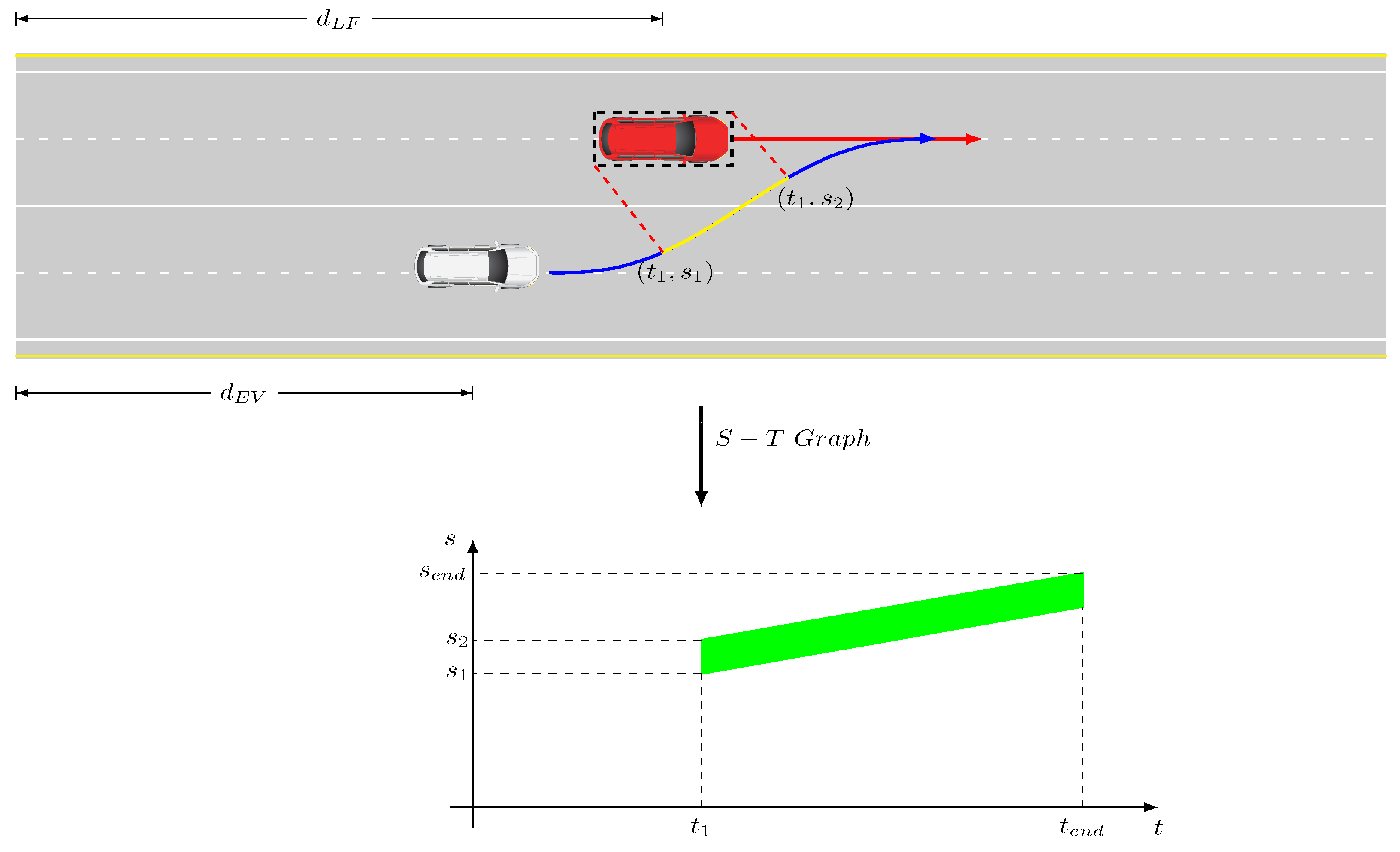
During the lane-changing process, the vehicle needs to adjust its driving strategy according to its surrounding environment. The whole lane-changing process is divided into two stages for considering the rear and front vehicles in the current and target lanes, respectively. The S–T graph is an efficient way to represent the configuration of the surrounding vehicles in the s and t dimensions. The S–T graph for a typical lane-changing scenario is shown in Figure 6 and if $d_{EV}>d_{LF}-0.5L-safedistance$, with L as the vehicle length, the effect that LF (red vehicle) has on the trajectory of the EV (white vehicle) should be taken into account. As shown in Figure 6, if at $t_1$ there is a latent collision, the inflated rectangle of the LF will be projected onto the trajectory of the EV and subsequently take up the range between $s_1$ and $s_2$ (green rectangle area). $s_{end}$ and $t_{end}$ are the length of the trajectory and the planning time, respectively.

Next, the space is sampled into discrete intervals in both the s and t dimensions, as shown in Figure 7, and DP is applied for deriving the optimal path (red dashed line), which consists of the minimal cost of every sample point in the space.

The cost function designed for each sample point in the space includes the cost of distance to the obstacle vehicle, cost of acceleration, desired speed and jerk.

$$J_{dp}={\omega }_{1}cos{t}_{obs}+{\omega }_2{\left(\ddot{s}\right)}^2+{\omega }_3{\left(\stackrel{⃛}{s}\right)}^2+{\omega }_4{(\dot{s}-v_{desired})}^2$$

(36)

The cost of distance to the obstacle vehicle is based on the distance from the COM of the EV to the line segment of each edge of the inflated rectangle, which represents the obstacle vehicle. The vector from the COM of the EV to the starting point of the line segment is $\overrightarrow{v_1}$ and to the ending point of the line segment is $\overrightarrow{v_2}$; the vector representing the line segment is $\overrightarrow{v_3}$. Then, the distance from the COM of the EV to the line segment can be calculated using (37). After calculating the four line segments of the rectangle, the distance is the minimum one.

$$mindistance=\left\{\begin{array}{cc}min(|\overrightarrow{v_1}|,|\overrightarrow{v_2}|)\hfill & \mathrm{if}sign(\overrightarrow{v_1}·\overrightarrow{v_3})=sign(\overrightarrow{v_2}·\overrightarrow{v_3})\hfill \\ \frac{|\overrightarrow{v_1}\times \overrightarrow{v_3}|}{|\overrightarrow{v_3}|}\hfill & \mathrm{otherwise}\hfill \end{array}\right.$$

(37)

The DP solution is a rough solution for the final speed profile and it will create a searching space for the QP framework as shown in Figure 8. The QP takes the constraints implemented by the search space and physical limitations, etc. The elements needed for the QP framework are shown in (38) and (39). The constraints for s and $\dot{s}$ are imposed by the obstacle vehicle and the speed limit of the lane. Since the S–T graph is constructed based on the planned path, the lateral acceleration is related to the curvature of the planned path. After the QP solution of speed profile is obtained, it will be combined with the planned path as a whole and sent to the control layer for tracking control.

$$constraints=\left\{\begin{array}{c}{s}_i\in [s_{lb}\left(t_i\right),s_{ub}\left(t_i\right)]\hfill \\ {\dot{s}}_i\in [0,\sqrt{\frac{a_{ymax}}{\kappa }}]\hfill \\ \ddot{s_i}\in [{\ddot{s}}_{lb}\left(t_i\right),{\ddot{s}}_{ub}\left(t_i\right)]\hfill \\ s_i<=s_{i+1}\hfill \\ s_{i+1}=s_i+\dot{s_i}dt+\frac{1}{2}\ddot{s_i}d{t}^2+\frac{1}{6}({\ddot{s}}_{i+1}-{\ddot{s}}_i)d{t}^2\hfill \\ {\dot{s}}_{i+1}=\dot{s_i}+\ddot{s_i}dt+\frac{1}{2}({\ddot{s}}_{i+1}-{\ddot{s}}_i)dt\hfill \end{array}\right.$$

(38)

$$J_{qp}={\omega }_1\sum _{i=1}^{N_s}{(\dot{s_i}-v_{desired})}^2+{\omega }_2\sum _{i=1}^{N_s}{\left(\ddot{s_i}\right)}^2+{\omega }_3\sum _{i=1}^{N_s}{\left(\stackrel{⃛}{s_i}\right)}^2$$

(39)

5. Trajectory Tracking Controller Design

5.1. Vehicle Modeling

A vehicle dynamics model that reflects the vehicle characteristics is a decisive factor to determine the quality of trajectory planning and motion control for an AV. There are many different kinds of vehicle models according to research objectives [52]. Although higher precision for trajectory planning and motion control is acquired by a vehicle dynamics model with more degrees of freedom (DOF), this will increase the cost for computation and decrease the convergence speed for algorithms. Therefore, some reasonable assumptions are made as follows [33]:

(1)

The vehicles are assumed to drive along a flat road, therefore ignoring vertical movement.

(2)

The suspension system and the vehicle are rigid bodies, therefore ignoring the suspension motion and its influence on the coupling relationship.

(3)

A fixed transmission ratio is assumed, which means the steering wheel angle input is applied on the wheels directly.

(4)

The moment of inertia of the vehicle model is constant and the COM cannot move for the lateral load transfer.

(5)

The influences of longitudinal and lateral aerodynamics are ignored.

(6)

We only consider the tire-cornering characteristics and ignore the coupling relationship of the longitudinal and lateral tire forces.

(7)

A small-angle assumption is made for the steering angle.

(8)

The vehicle travels with a constant longitudinal velocity in the vehicle body coordinate system.

5.2. Vehicle Dynamics

Based on the previous assumptions, the actual vehicle can be simplified into a two-DOF bicycle model, which only considers two directions of motion, i.e., lateral and yaw motions; see Figure 9. The coordinate system OXYZ represents the geodetic coordinate system, while OXYZ is the vehicle body coordinate system in which o is the COM, and both coordinate systems follow the right-hand rule. Moreover, the three directions of motion refer to longitudinal motion along the x axis, lateral motion along the y axis and yaw motion around the z-axis, which is perpendicular to the oxy plane.

Let us define $v_c$ as the velocity of the COM according to the instant center of the vehicle with a certain rotation radius, $\phi$ as the yaw angle between the axial line of the vehicle and the X axis, $\beta$ as the side slip angle of the COM between the velocity of the COM and the x axis, and $\phi$ + $\beta$ as the heading angle between the velocity of the COM and the X axis; $L_r$ and $L_f$ are the lengths between the COM and the rear wheel and front wheel, respectively; L = $L_r$ + $L_f$ is the wheel base and ${\delta }_f$ is the front wheel angle. In the case of low-speed scenarios, it is assumed that only the front wheel can be steered; therefore, $\beta \approx 0$ and ${\delta }_r\approx 0$. After some basic geometric manipulations, the kinematics characteristic is expressed as:

$$\dot{X}=v_{c}cos\phi$$

(40)

$$\dot{Y}=v_{c}sin\phi$$

(41)

$$\dot{\phi }=\frac{v_{c}tan{\delta }_f}{L}$$

(42)

As can be seen in the above equations, the kinematics characteristic has the property of nonlinearity and the coupling effect between $v_c$ and ${\delta }_f$, which makes it inappropriate for the motion controller design in the longitudinal and lateral directions. Therefore, it will be applied for the coordinate transformation between the Cartesian and Frenet frames described later.

In order to overcome the limitations of the kinematics model for high-speed scenarios, the property of the tires should be included in the modeling process, which will be presented in the vehicle dynamics model.

For the front steering vehicle based on the small-angle assumption, the lateral tire force can be linearized as follows:

$$F_{yf}=C_f{\alpha }_f$$

(43)

$$F_{yr}=C_r{\alpha }_r$$

(44)

where $C_f$ and $C_r$ are the cornering stiffness values of the front and rear tires, respectively, which are always negative values according to the right-hand rule, and ${\alpha }_f$ and ${\alpha }_r$ are the side slip angles of the front and rear tires.

According to Newton’s second law, the force analysis is carried out based on the force and moment balance, which establishes the following dynamic equations:

$$m{a}_y=F_{yf}cos{\delta }_f+F_{yr}$$

(45)

$$I_z\ddot{\phi }=F_{yf}cos{\delta }_f{L}_f-F_{yr}{L}_r$$

(46)

where m is the mass of the vehicle and $I_z$ represents the moment of inertia around the z axis.

The absolute acceleration component of the vehicle COM along the y axis is expressed as

$$a_y=\ddot{y}+v_{cx}\dot{\phi }$$

(47)

The side slip angles of the front and rear wheels can be approximately expressed as follows based on the small-side-slip-angle assumption:

$${\alpha }_f=\frac{\dot{\phi }{L}_f+v_{cy}}{v_{cx}}-{\delta }_f$$

(48)

$${\alpha }_r=\frac{v_{cy}-\dot{\phi }{L}_r}{v_{cx}}$$

(49)

Substituting Equations (43), (44), (47), (48) and (49) into (45) and (46) while considering $cos{\delta }_f\approx 1$ results in:

$$m({\dot{v}}_{cy}+v_{cx}\dot{\phi })=C_f(\frac{\dot{\phi }{L}_f+v_{cy}}{v_{cx}}-{\delta }_f)+C_r(\frac{v_{cy}-\dot{\phi }{L}_r}{v_{cx}})$$

(50)

$$I_z\ddot{\phi }=L_f{C}_f(\frac{\dot{\phi }{L}_f+v_{cy}}{v_{cx}}-{\delta }_f)-L_r{C}_r(\frac{v_{cy}-\dot{\phi }{L}_r}{v_{cx}})$$

(51)

Furthermore, (50) and (51) can be translated into the state space model with $x={[\dot{y},\dot{\phi }]}^T$ and $u={\delta }_f$ as:

$$\dot{x}=Ax+Bu$$

(52)

with A and B as:

$$A=\left[\begin{array}{cc}\frac{C_f+C_r}{m{v}_{cx}}& \frac{L_f{C}_f-L_r{C}_r}{m{v}_{cx}}-v_{cx}\\ \frac{L_f{C}_f-L_r{C}_r}{I_z{v}_{cx}}& \frac{L_f^2{C}_f+L_r^2{C}_r}{I_z{v}_{cx}}\end{array}\right]$$

(53)

$$B=\left[\begin{array}{c}-\frac{C_f}{m}\\ -\frac{L_f{C}_f}{I_z}\end{array}\right]$$

(54)

5.3. Tracking Error Model

Trajectory tracking is mainly about controlling the vehicles to track a planned reference trajectory stably and rapidly [53]. In order to facilitate the controller design for trajectory tracking, the tracking error model should be used. Similar to Figure 4, with the reference line being replaced by the reference trajectory, let $Q=(x,y)$ be the vehicle’s position and the projection point of the vehicle on the reference trajectory be $P=(x_r,y_r)$. According to the projection point P, s is the curvilinear distance along the reference trajectory and the unit tangent vector, unit normal vector and velocity vector are built, which are $\overrightarrow{{\tau }_r}$, $\overrightarrow{n_r}$ and $\overrightarrow{\dot{s}}$, respectively. The lateral error is $e_y=\left|\overrightarrow{PQ}\right|$, while the desired heading angle and the actual heading angle are ${\theta }_r$ and ${\theta }_h=\phi +\beta$, respectively. Therefore, the heading error is ${\theta }_h-{\theta }_r$. The unit direction vector of the velocity vector of the vehicle’s COM $\overrightarrow{v_h}$ is $\overrightarrow{{\tau }_h}$ and its unit normal vector is $\overrightarrow{n_h}$.

According to the geometric relations, the lateral error is $e_y=(\overrightarrow{OQ}-\overrightarrow{OP})·\overrightarrow{n_r}$. Considering that $\overrightarrow{n_r}$ is not a constant vector and taking the derivative of both sides of the equation, we obtain

$$\dot{e_y}=(\overrightarrow{\dot{OQ}}-\overrightarrow{\dot{OP}})·\overrightarrow{n_r}+(\overrightarrow{OQ}-\overrightarrow{OP})·\overrightarrow{\dot{n_r}}$$

(55)

The real and desired position vector can be expressed as:

$$\overrightarrow{\dot{OQ}}=\left|\overrightarrow{v_h}\right|\overrightarrow{{\tau }_h}$$

(56)

$$\overrightarrow{\dot{OP}}=\left|\overrightarrow{\dot{s}}\right|\overrightarrow{{\tau }_r}$$

(57)

Let us define $e_{\phi }=\phi -{\theta }_r$, which is small based on the assumption. Then, let us substitute (56) and (57) into (55) while considering the Serret–Frenet equation; then, we obtain:

$$\dot{e_y}=v_{cx}sin{e}_{\phi }+v_{cy}cos{e}_{\phi }$$

(58)

Omitting the large curvature of the trajectory scenarios, a group of equations from (58) is obtained:

$$v_{cy}=\dot{e_y}-v_{cx}{e}_{\phi }$$

(59)

$$\dot{v_{cy}}=\ddot{e_y}-v_{cx}\dot{e_{\phi }}$$

(60)

$$\dot{\phi }=\dot{e_{\phi }}+\dot{{\theta }_r}$$

(61)

$$\ddot{\phi }=\ddot{e_{\phi }}$$

(62)

Choosing the state as $x_e={[\dot{e_y},\ddot{e_y},\dot{e_{\phi }},\ddot{e_{\phi }}]}^T$ and combining with the previous vehicle dynamics model results in the following state-space tracking error model:

$$\dot{x_e}=A_e{x}_e+B_{e}u+C_e\dot{{\theta }_r}$$

(63)

and $A_e$, $B_e$ and $C_e$ are:

$$A_e=\left[\begin{array}{cccc}0& 1& 0& 0\\ 0& \frac{C_f+C_r}{m{v}_{cx}}& -\frac{C_f+C_r}{m}& \frac{L_f{C}_f-L_r{C}_r}{m{v}_{cx}}\\ 0& 0& 0& 1\\ 0& \frac{L_f{C}_f-L_r{C}_r}{I_z{v}_{cx}}& -\frac{L_f{C}_f-L_r{C}_r}{I_z}& \frac{L_f^2{C}_f+L_r^2{C}_r}{I_z{v}_{cx}}\end{array}\right]$$

(64)

$$B_e=\left[\begin{array}{c}0\\ -\frac{C_f}{m}\\ 0\\ -\frac{L_f{C}_f}{I_z}\end{array}\right]C_e=\left[\begin{array}{c}0\\ \frac{L_f{C}_f-L_r{C}_r}{m{v}_{cx}}-v_{cx}\\ 0\\ \frac{L_f^2{C}_f+L_r^2{C}_r}{I_z{v}_{cx}}\end{array}\right]$$

(65)

5.4. LQR Controller Design

Based on the lateral error $e_y$ and the deviation of yaw angle $e_{\phi }$, the LQR controller provides the vehicle with the steering angle in an optimal way.

The previous tracking error model should be converted to a discrete form to obtain the LQR control law. The term $\dot{{\theta }_r}$ is omitted here (it will be considered later). Using the midpoint Euler method, the model is discretized with sampling time T as follows:

$$\begin{array}{cc}\hfill & x_e(k+1)=\overline{A_e}{x}_e\left(k\right)+\overline{B_e}u\left(k\right)\hfill \\ \hfill & ={(I-\frac{A_{e}T}{2})}^{-1}(I+\frac{A_{e}T}{2})x_e\left(k\right)+B_{e}Tu\left(k\right)\hfill \end{array}$$

(66)

The discretized state space model (66) is considered as the constraint in the following objective function:

$$J=\sum _{k=0}^{\infty }\left\{{x_e\left(k\right)}^{T}Q{x}_e\left(k\right)+{u\left(k\right)}^{T}Ru\left(k\right)\right\}$$

(67)

Therefore, applying the Lagrangian multiplier method, the optimal control law $u\left(k\right)=-K{x}_e\left(k\right)$ can be obtained as:

$$P=Q+{\overline{A_e}}^{T}P\overline{A_e}-{\overline{A_e}}^{T}P\overline{B_e}{(R+{\overline{B_e}}^{T}P\overline{B_e})}^{-1}{\overline{B_e}}^{T}P\overline{A_e}$$

(68)

$$K={(R+{\overline{B_e}}^{T}P\overline{B_e})}^{-1}{\overline{B_e}}^{T}P\overline{A_e}$$

(69)

5.5. Feedforward Control

In the previous section, the term $\dot{{\theta }_r}$ was ignored to derive the optimal control of LQR. However, it can be seen from the following that the steady-state error will not be zero:

$$\dot{x_e}=(A_e-B_{e}K)x_e+C_e\dot{{\theta }_r}$$

(70)

Therefore, the feedforward control law is integrated into the LQR as follows to eliminate the steady-state error:

$$u=-K{x}_e+{\delta }_f$$

(71)

After introducing the feedforward control and by setting $\dot{x_e}=0$, the steady-state error is expressed as

$$x_e={(A_e-B_{e}K)}^{-1}(B_e{\delta }_f+C_e\dot{{\theta }_r})$$

(72)

The exact expression of $x_e$ can be obtained using the scientific computing software Mathematica as follows:

$$x_e=\left[\begin{array}{c}\frac{1}{k_1}\left\{{\delta }_f-\frac{\dot{{\theta }_r}}{v_{cx}}\left[L_f+L_r-L_r{k}_3-\frac{m{v}_{cx}^2}{Lf+Lr}\left(\frac{L_r}{C_f}+\frac{L_f}{C_r}{k}_3-\frac{L_f}{C_r}\right)\right]\right\}\\ 0\\ -\frac{\dot{{\theta }_r}}{v_{cx}}\left(L_r+\frac{L_f}{L_f+L_r}\frac{m{v}_{cx}^2}{C_r}\right)\\ 0\end{array}\right]$$

(73)

where $K=[k_1,k_2,k_3,k_4]$ and $\dot{e_y}=0$ when

$${\delta }_f=\frac{\dot{{\theta }_r}}{v_{cx}}\left[L_f+L_r-L_r{k}_3-\frac{m{v}_{cx}^2}{Lf+Lr}\left(\frac{L_r}{C_f}+\frac{L_f}{C_r}{k}_3-\frac{L_f}{C_r}\right)\right]$$

(74)

It can be seen that $e_{\phi }=-\frac{\dot{{\theta }_r}}{v_{cx}}\left(L_r+\frac{L_f}{L_f+L_r}\frac{m{v}_{cx}^2}{C_r}\right)$ seems not to be controlled by ${\delta }_f$ and K. However, based on the previous assumption, the expression of $e_{\phi }$ can be reduced to $e_{\phi }=-\beta$, which means the heading error $\theta -{\theta }_r=0$ and verifies the definition $e_{\phi }=\phi -{\theta }_r\Rightarrow -\beta =\phi -{\theta }_r\Rightarrow \phi +\beta ={\theta }_r$.

5.6. Discrete Trajectory-Error Calculation

From the previous section, it can be seen that in order to calculate the state error, the coordinate of projection point P of the vehicle position p under the Cartesian frame is needed. Since the position, velocity and yaw rate are available from the sensor system, only the unknowns $x_r,y_r,{\theta }_r$ and $\kappa$ are left.

It is worth noting that if the planned trajectory is continuous, the projection point of the vehicle position on the trajectory may not be unique (e.g., if the reference trajectory is circular and the vehicle position is at the center).

Therefore, the trajectory planned in this paper is the set of a series of discrete waypoints. The process of calculating the state error is summarized as follows. First, find the point $L_m$ with the max index in the waypoint set that has the shortest distance to the vehicle position. The information included in $L_m$ is $(x_m,y_m,{\theta }_m,{\kappa }_m)$.

Then, in order to find the projection point, the assumption is that the curvatures at $L_m$ and $L_p$ are the same, which means that an arc is a proper substitution for the trajectory between these two points.

Finally, the following equations are derived from Figure 4:

$$e_y=(\overrightarrow{x}-\overrightarrow{x_m})·\overrightarrow{n_m}$$

(75)

$$e_s=(\overrightarrow{x}-\overrightarrow{x_m})·\overrightarrow{{\tau }_m}$$

(76)

$${\theta }_r={\theta }_m+{\kappa }_m{e}_s$$

(77)

$${\kappa }_r={\kappa }_m$$

(78)

5.7. Longitudinal Controller

The longitudinal controller is implemented with a double PID controller, which is shown in Figure 10. The inputs of the PID controller are the reference state from the trajectory-planning module and the vehicle state from the CarSim vehicle model. The inverse model consists of the inverse powertrain model and the inverse-brake-system model. After receiving the controlling signal from the PID controller, the inverse model will transform the controlling signal into throttle or brake, send it to the CarSim vehicle model and generate the updated vehicle state.

The throttle angle (${\alpha }_t$) and the braking pressure ($P_b$) are

$$\begin{array}{c}\hfill T_{edes}=\frac{(m{a}_{pid}+mgf+C_d{v}^2)}{{\eta }_t{i}_g{i}_f}r\\ \hfill {\alpha }_t=MA{P}^{-1}({\omega }_e,T_{edes})\\ \hfill P_b=\frac{(m{a}_{pid}+C_d{v}^2+mgf)}{K_b}\end{array}$$

(79)

where MAP(•) is a nonlinear tabular function representing engine torque characteristics, $a_{pid}$ is the output of the double PID controllers, m is the vehicle mass, $i_g$ is the gear ratio, $i_f$ is the ratio of the final gear, ${\omega }_e$ is the engine speed, r is the rolling radius of the wheels, g is the gravity coefficient, f is the coefficient of the rolling resistance, $C_d$ is the coefficient of the aerodynamic drag, v is the vehicle velocity, $K_b$ is the total braking gain of the wheels and ${\eta }_t$ is the mechanical efficiency of the driveline.

6. Simulation and Results

The proposed framework was implemented on the co-simulation platforms MATLAB/Simulink R2020a, PreScan8.5 and CarSim 2020, as shown in Figure 11. The four scenarios were constructed in PreScan, which provides the driving environment including the road information, surrounding vehicles and EV information; the main part of the proposed framework was implemented in MATLAB/Simulink, which connects PreScan and CarSim, as it receives the driving environment information from PreScan and sends the control signal to CarSim, while CarSim provides the high-definition vehicle model and sends the updated state information to PreScan.

The simulation parameters are shown in

Table 2. Parameters in simulation.

Parameters	Value
Vehicle mass m (kg)	2020
Vehicle moment of inertia $I_z$ (kg·m${}^2$)	4095
Distance between COM and front wheel $L_f$ (m)	1.265
Distance between COM and rear wheel $L_r$ (m)	1.682
Cornering stiffness of the front tires $C_f$ (N/rad)	−175,016
Cornering stiffness of the rear tires $C_r$ (N/rad)	−130,634
Trajectory-planning simulation period $T_p$ (s)	0.1
Controller simulation period $T_c$ (s)	0.01

. The planning module will work at a frequency of 10 Hz since the vehicle state will not change too much during the short updated period and a higher frequency will consume more computing resources. However, the control module works at a frequency of 100 Hz since the control task needs to be performed at a higher frequency than the planning module in order to ensure the accuracy, safety and comfort of the trajectory tracking [54]. In order to further reduce the computation burden of the simulation platform, the LQR controller gain is calculated offline in advance, which creates a lookup table covering the simulation scenarios under different velocities ranging from 0.01 m/s to 50 m/s, with an interval of 0.01 m/s.

It should be noted that labeled vehicles such as LR, LF, CF, RF and RR may change during the simulation process. For example, the CF vehicle may change to the RR vehicle or the LR vehicle after the left lane-changing or right lane-changing behavior. Therefore, the label used for the surrounding vehicle is based on the initial relative position of the EV and surrounding vehicles.

The testing road constructed in PreScan is a three-lane road, which consists of a straight section and a curved section. The centerline coordinate of the middle lane starts with (0, 0) and the counterparts of the left lane and right lane are 3.5 m in the positive and negative directions of the y axis, respectively. The proposed trajectory planning and controller are expected to track the reference trajectory as closely as possible. The centerline of the middle lane is shown in Figure 12a, and the effectiveness of the controller is validated through the acceleration, $e_y$, $e_{\phi }$, $e_s$ and the velocity of the EV as shown in Figure 12b–f. The desired velocity is 25 m/s and the tracking error is within the acceptable region, and it can be concluded that the proposed trajectory planning and tracking controller are capable of tracking the reference trajectory while keep the desired velocity as much as possible in the curved road.

In the first scenario, the simple lane-changing scenario is simulated, as shown in Figure 13. The EV is driving with an initial speed of 20 m/s at position (250, 0), its desired speed is 25 m/s and the adjacent lanes are empty. The CF vehicle is located at (300, 0) and the lane-changing command is generated after the preceding vehicle moves slower than the desired speed. At first, the velocity of the preceding vehicle is 25 m/s and at around the third second the preceding vehicle starts to decelerate, as shown in Figure 13. After the minimum safe distance is reached, the sensor detects the slower preceding vehicle and finds the left lane is empty; the left-lane-change command is generated to reach the desired velocity. The results show that the controller can guarantee a smooth lane-change maneuver, which is represented by the yaw angle, yaw rate and steering angle. One can also see from the planned trajectory and the tracking process in the figure that there is not much overshooting during the process. After the lane change is completed, the EV performs the overtaking maneuver to maintain its desired velocity, which shows the feasibility of the proposed framework.

The second scenario simulation result is shown in Figure 14; there is an LR in the left lane located at (220, 3.5). The EV is at (250, 0) and the CF position is (300, 0), and both vehicles possess similar speed profiles to the first scenario. The LR starts with the initial velocity of 20 m/s and lies 30 m behind the EV, while the CF starts with an initial velocity of 25 m/s and lies 50 m ahead. The CF starts to brake harshly and the LR starts to accelerate around the fourth second and after the minimum distance with the CF is reached, the left lane-change command is generated around the seventh second when the left lane is safe. However, during the lane-changing process, the left lane is not safe anymore due to the acceleration of the LR; the EV decides to change back to its original lane and after around 3 s it returns to the car-following maneuver. Then, the EV finds the right lane is empty and performs a right-lane change, finally reaching the desired velocity of 25 m/s.

In the third scenario, the positions for the EV, RF, LF and CF are (250, 0), (319.991, −2.9899), (280, 3.5) and (349.869, 3.1322), respectively, and the simulation results are shown in Figure 15. The EV starts with the initial velocity of 20 m/s and its desired velocity is 25 m/s; the CF starts with an initial velocity of 18 m/s and lies 100 m ahead, while the LF starts with an initial velocity of 21 m/s and lies 30 m ahead in the left lane, and there is also an RF which starts with an initial velocity of 15 m/s and lies 70 m ahead. The safe condition is satisfied at the start, which guarantees the free-driving maneuver of the EV; at around the sixth second, the driving state changes to car following due to the slower CF and unsafe left lane and right lane. The left-lane-change signal is generated at around the tenth second due to the faster LF in the adjacent lane and the safe distance is reached. Since the LF is slower than the desired velocity, another car-following maneuver is performed at around the fifteenth second, and after around 5 s the EV starts to change to the middle lane due to the safe distance from the previous current-lane vehicle and reaches the desired velocity of 25 m/s. This case shows that the proposed framework could generate a reasonable driving strategy adaptively for the EV to seek the desired velocity while maintaining road safety by automatically switching between different driving states.

In the fourth scenario, a more complex driving environment is implemented. The EV starts at (0, 0) with an initial desired velocity of 25 m/s, and there are six vehicles around it corresponding to positions sedan2 (20, 3.5), sedan3 (40, −3.5), sedan4 (40, 0), sedan5 (30, 3.5), sedan6 (50, −3.5) and sedan7 (50, 0), traveling at speeds of 18 m/s, 15 m/s, 20 m/s, 22 m/s, 20 m/s and 20 m/s, respectively. The simulation results are shown in Figure 16. During the first 4 s, the EV is free driving and after the safe distance limit is reached with respect to sedan4, the EV decelerates to change to the car-following state. At around the eighth second, sedan5 decelerates to about 19 m/s while sedan6 reaches about 21.5 m/s, which means a potential faster right lane to reach the desired speed. Hence, the EV performs the right-lane-change maneuver and drives freely since the safe distance from sedan6 is still ensured. At around the tenth second, when the safe distance between the EV and sedan6 decreases to the threshold, the EV starts to follow sedan6. However, the relative distance between sedan7 and the EV is expanding due to the acceleration of sedan7 during this time. When the middle lane is safe for a lane change at around the twenty-first second, the EV performs the left lane change to pursue the desired speed. During the process, the EV accelerates first to finish the lane change and switch to car following again due to the safe distance diminishing. At around the twenty-sixth second, the EV performs another left-lane-change maneuver to finally reach the desired speed. This case further illustrates the effectiveness of the proposed framework, which guides the vehicle to drive safely at the desired velocity as best as possible under the complex surrounding environment.

7. Conclusions

In this paper, we proposed a novel framework combining decision-making, trajectory-planning and tracking control schemes for AVs based on the state machine for intelligent decision making and LQR and PID controllers for trajectory tracking. The state machine is proposed for the decision making of the AV (free driving, car following, and lane changing) adaptively to ensure driving safety and achieve the expected velocity requirements. The LQR and PID controllers are responsible for tracking the planned trajectory based on quintic polynomials and conduct car-following or lane-change maneuvers according to the command of the finite-state machine. A comprehensive scenario-study analysis, including both straight and curved roads, was conducted to evaluate the performance of the proposed framework. The results demonstrate that the proposed framework has reasonable performance in the simulation scenarios. The framework was able to guide the vehicle in driving safely under complex driving environments while maintaining its ability to pursue the desired velocity as much as possible.

Future work will be directed toward decision making and motion planning for different driving styles. For example, the desired velocity was preset manually in this study and the method can be improved if the desired velocity can be decided according to different driving conditions and driving styles. Some artificial-intelligence (AI) technologies such as deep learning or reinforcement learning [55] can be implemented to improve the intelligence of the decision and planning framework by learning driving principles and styles from real driving data. Furthermore, the proposed framework needs to be generalized to be suitable for other common studies on structured driving environments, such as highway merging, unsignalized intersections, and roundabouts, etc. However, the challenge lies in the formulation of these complex scenarios, and the performance of the framework needs to be validated by taking diverse driving characteristics into account, which will be the focus of future research.